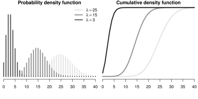
Poisson regression

\[ p(Y_i) = \frac{e^{-\lambda}\lambda^x}{x!} \]

\[log(\mu)=\beta_0+\beta_1x_i+...+\beta_px_p\]

Dispersion

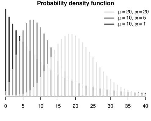
Spread assumed to be equal to mean. (\(\phi = 1\))

Dispersion

Over-dispersion

Sample more varied than expected from its mean

variability due to other unmeasured (latent) influences
- quasi-poisson model
- negative binomial
- observation level random effect

Dispersion

Over-dispersion

Sample more varied than expected from its mean

variability due to other unmeasured (latent) influences
clumpiness
- negative binomial model
due to more zeros than expected
- zero-inflated model

Residuals

difficult to interpret

Simulated Residuals

residuals uniform when model good

Simulated Residuals

residuals uniform when model good

Simulated Residuals

residuals uniform when model good

Simulated Residuals

residuals uniform when model good

Poisson regression 1

Quasi-Poisson

specify \(var(y) = \phi \mu\)
\(\phi\) (scale parameter) estimated
parameter estimates same
Standard errors \(=\sqrt{\phi}\times SE\)

Quasi-Poisson

Negative Binomial

\[p(y_i)=\frac{\Gamma(y_i+\omega)}{\Gamma(\omega)y!}\times\frac{\mu_i^{y_i}\omega^\omega}{(\mu_i+\omega)^{\mu_i+\omega}}\]

Negative Binomial

\[p(y_i)=\frac{\Gamma(y_i+\omega)}{\Gamma(\omega)y!}\times\frac{\mu_i^{y_i}\omega^\omega}{(\mu_i+\omega)^{\mu_i+\omega}}\]

mixture model
\(\eta_i \sim Gamma(\mu_i, \omega)\)
\(E(y) \sim Poisson(\eta_i)\)

Worked Example

Zero-inflated model

Two sources of zeros
- those expected by Poisson (or binomial)
- false zeros

Mixture model
- binary logistic (rate of false zeros)
- Poisson (trend in counts)

Worked Example

Observation-level random effects

Worked Examples

Format of quinn.csv data files

SEASON	DENSITY	RECRUITS	SQRTRECRUITS	GROUP
Spring	Low	15	3.87	SpringLow
..	..	..	..	..
Spring	High	11	3.32	SpringHigh
..	..	..	..	..
Summer	Low	21	4.58	SummerLow
..	..	..	..	..
Summer	High	34	5.83	SummerHigh
..	..	..	..	..
Autumn	Low	14	3.74	AutumnLow
..	..	..	..	..

SEASON	Categorical listing of Season in which mussel clumps were collected independent variable
DENSITY	Categorical listing of the density of mussels within mussel clump independent variable
RECRUITS	The number of mussel recruits response variable
SQRTRECRUITS	Square root transformation of RECRUITS - needed to meet the test assumptions
GROUPS	Categorical listing of Season/Density combinations - used for checking ANOVA assumptions

  SEASON DENSITY RECRUITS SQRTRECRUITS      GROUP
1 Spring     Low       15     3.872983  SpringLow
2 Spring     Low       10     3.162278  SpringLow
3 Spring     Low       13     3.605551  SpringLow
4 Spring     Low       13     3.605551  SpringLow
5 Spring     Low        5     2.236068  SpringLow
6 Spring    High       11     3.316625 SpringHigh

moths

Format of moth.csv data files

METERS	A	P	HABITAT
25	9	8	NWsoak
37	3	20	SWsoak
109	7	9	Lowerside
10	0	2	Lowerside
133	9	1	Upperside
26	3	18	Disturbed

METERS	The length of the section of transect
A	The number of moth species A observed in section of transect
P	The number of moth species P observed in section of transect
HABITAT	Categorical listing of the habitat type within section of transect.

  METERS A  P   HABITAT
1     25 9  8    NWsoak
2     37 3 20    SWsoak
3    109 7  9 Lowerside
4     10 0  2 Lowerside
5    133 9  1 Upperside
6     26 3 18 Disturbed

[1] 6.735895e-07

[1] 0.175419

[1] 0

[1] 0.04489437

[1] 2.700801

[1] 1.228093

[1] 8.843367

[1] 1.452578

[1] 2.93723

[1] 5.462792

[1] 1.455681

[1] 1.371939


FALSE  TRUE 
 0.85  0.15


FALSE  TRUE 
0.994 0.006

             df     AICc
moths.glmO    7 312.4946
moths.glmC    8 229.3589
moths.glmNBO  8 233.1423
moths.glmNBC  9 213.2019


Call:
glm.nb(formula = A ~ log(METERS) + HABITAT, data = moths, init.theta = 4.195676174, 
    link = log)

Deviance Residuals: 
    Min       1Q   Median       3Q      Max  
-2.4806  -1.2400  -0.0062   0.6398   1.9712  

Coefficients:
                 Estimate Std. Error z value Pr(>|z|)    
(Intercept)       -0.1076     0.4589  -0.235  0.81455    
log(METERS)        0.1451     0.1372   1.057  0.29041    
HABITATLowerside   1.2864     0.4710   2.731  0.00631 ** 
HABITATNEsoak      0.4293     0.5858   0.733  0.46369    
HABITATNWsoak      2.8306     0.5392   5.250 1.52e-07 ***
HABITATSEsoak      1.3327     0.5092   2.617  0.00887 ** 
HABITATSWsoak      1.4899     0.5981   2.491  0.01274 *  
HABITATUpperside   1.0764     0.6979   1.542  0.12299    
---
Signif. codes:  0 '***' 0.001 '**' 0.01 '*' 0.05 '.' 0.1 ' ' 1

(Dispersion parameter for Negative Binomial(4.1957) family taken to be 1)

    Null deviance: 105.899  on 39  degrees of freedom
Residual deviance:  46.582  on 32  degrees of freedom
AIC: 207.2

Number of Fisher Scoring iterations: 1

              Theta:  4.20 
          Std. Err.:  1.96 

 2 x log-likelihood:  -189.202

    HABITAT METER       fit      lower     upper
1 Disturbed  45.5  1.562453  0.5638782  4.329411
2 Lowerside  45.5  5.655624  3.0673703 10.427850
3    NEsoak  45.5  2.400197  1.2093558  4.763650
4    NWsoak  45.5 26.492966 13.6799769 51.306904
5    SEsoak  45.5  5.923526  3.4228572 10.251134
6    SWsoak  45.5  6.931826  3.3129525 14.503741

Error in eval(expr, envir, enclos): could not find function "ggplot"

Workshop 10.6a: Poisson regression

Murray Logan

12 Sep 2016

Poisson regression

Poisson regression

Dispersion

Dispersion

Over-dispersion

Dispersion

Over-dispersion

Residuals

Simulated Residuals

Simulated Residuals

Simulated Residuals

Simulated Residuals

Worked Examples

Poisson regression 1

Quasi-Poisson

Quasi-Poisson

Quasi-Poisson

Negative Binomial

Negative Binomial

Worked Example

Zero-inflated model

Worked Example

Observation-level random effects

Reanalysis of earlier data sets

Worked Examples

Worked example

moths