General linear models

\[ Residual_i = y_i - E(Y_i) \]
\[\underbrace{E(Y)}_{Link~~function} = \underbrace{\beta_0 + \beta_1x_1~+~...~+~\beta_px_p}_{Systematic} + \varepsilon, ~~\varepsilon\sim Dist(...)\]

\[E(Y) = \left(\begin{array}{c} n\\x \end{array}\right)p^{x}(1-p)^{n-x}\]
Spread assumed to be equal to mean. (\(\phi = 1\))
polis <- read.csv('../data/polis.csv', strip.white=T)
head(polis)
ISLAND RATIO PA
1 Bota 15.41 1
2 Cabeza 5.63 1
3 Cerraja 25.92 1
4 Coronadito 15.17 0
5 Flecha 13.04 1
6 Gemelose 18.85 0ggplot(polis, aes(y=PA, x=RATIO))+geom_point()+
geom_smooth(method='glm', formula=y~x, family='binomial')Error: could not find function "ggplot"plot(PA~RATIO, data=polis )
abline(lm(PA~RATIO, data=polis))
with(polis,lines(lowess(PA~RATIO)))
polis.glm <- glm(PA ~ RATIO, family=binomial, data=polis)

par(mfrow=c(2,3))
plot(polis.glm)

##Check the model for lack of fit via:
##Pearson chisq
polis.resid <- sum(resid(polis.glm, type="pearson")^2)
1-pchisq(polis.resid, polis.glm$df.resid)
[1] 0.5715#No evidence of a lack of fit
#Deviance
1-pchisq(polis.glm$deviance, polis.glm$df.resid)[1] 0.6514#No evidence of a lack of fit
#Estimate dispersal
polis.resid/polis.glm$df.resid[1] 0.9019#OR
polis.glm$deviance/polis.glm$df.resid[1] 0.8365#Number of zeros
polis.tab<-table(polis$PA==0)
polis.tab/sum(polis.tab)
 FALSE   TRUE
0.5263 0.4737 summary(polis.glm)
Call:
glm(formula = PA ~ RATIO, family = binomial, data = polis)

Deviance Residuals:
   Min      1Q  Median      3Q     Max
-1.607  -0.638   0.237   0.433   2.099

Coefficients:
            Estimate Std. Error z value Pr(>|z|)
(Intercept)    3.606      1.695    2.13    0.033
RATIO         -0.220      0.101   -2.18    0.029

(Intercept) *
RATIO       *
---
Signif. codes:
0 '***' 0.001 '**' 0.01 '*' 0.05 '.' 0.1 ' ' 1

(Dispersion parameter for binomial family taken to be 1)

    Null deviance: 26.287  on 18  degrees of freedom
Residual deviance: 14.221  on 17  degrees of freedom
AIC: 18.22

Number of Fisher Scoring iterations: 6exp(-0.296)[1] 0.7438#R2
1-(polis.glm$deviance/polis.glm$null)[1] 0.459anova(polis.glm, test='Chisq')Analysis of Deviance Table
Model: binomial, link: logit
Response: PA
Terms added sequentially (first to last)
Df Deviance Resid. Df Resid. Dev Pr(>Chi)
NULL 18 26.3
RATIO 1 12.1 17 14.2 0.00051
NULL
RATIO ***
---
Signif. codes:
0 '***' 0.001 '**' 0.01 '*' 0.05 '.' 0.1 ' ' 1par(mar=c(4,5,0,0))
plot(PA~RATIO, data=polis,type="n",ann=F,axes=F)
points(PA~RATIO, data=polis,pch=16)
xs <- seq(min(polis$RATIO),max(polis$RATIO),len=1000)
ys <- predict(polis.glm,newdata=data.frame(RATIO=xs),
type='link',se=T)
ys$lwr <- polis.glm$family$linkinv(ys$fit - 2*ys$se.fit)
ys$upr <- polis.glm$family$linkinv(ys$fit + 2*ys$se.fit)
ys$fit <- polis.glm$family$linkinv(ys$fit)
lines(ys$fit~xs, col='black')
lines(ys$lwr~xs, col='black',lty=2)
lines(ys$upr~xs, col='black',lty=2)
axis(1)
mtext("Island perimeter to area ratio",1,cex=1.5,line=3)
axis(2,las=2)
mtext(expression(paste(italic(Uta)," lizard presence/absence")),2,cex=1.5,line=3)
box(bty="l")
#LD50
ld50<--polis.glm$coef[1]/polis.glm$coef[2]
newdata <- data.frame(RATIO=xs, fit=ys$fit, lower=ys$lwr, upper=ys$upr)
ggplot(newdata, aes(y=fit, x=RATIO))+geom_line()+
geom_ribbon(aes(ymin=lower, ymax=upper), fill='blue',alpha=0.2)+
geom_point(data=polis, aes(y=PA, x=RATIO))Error: could not find function "ggplot"
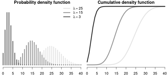
\[ p(Y_i) = \frac{e^{-\lambda}\lambda^x}{x!} \]
\[log(\mu)=\beta_0+\beta_1x_i+...+\beta_px_p\]
Spread assumed to be equal to mean. (\(\phi = 1\))
data.pois <- read.csv('../data/data.pois.csv', strip.white=T)
head(data.pois)
y x
1 1 1.025
2 2 2.697
3 3 3.626
4 2 4.949
5 4 6.025
6 8 6.254library(car)
scatterplot(y~x,data=data.pois)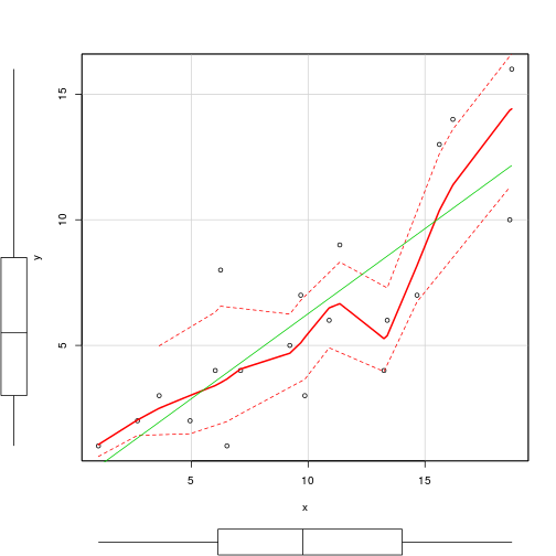
scatterplot(y~x,data=data.pois, log='y')
rug(jitter(data.pois$y), side=2)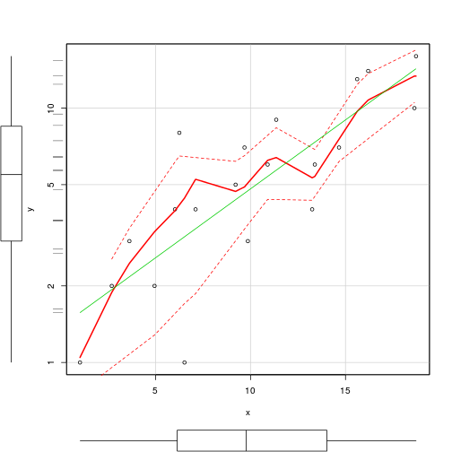
hist(data.pois$y)
boxplot(data.pois$y, horizontal=TRUE)
rug(jitter(data.pois$y), side=1)
#plot(y~x, data.pois, log="y")
#with(data.pois, lines(lowess(y~x)))
#library(car)
#scatterplot(y~x,data=data.pois, log='y')
#rug(jitter(data.pois$y), side=2)


#Zero inflation
#proportion of 0's in the data
data.pois.tab<-table(data.pois$y==0)
data.pois.tab/sum(data.pois.tab)
FALSE
    1
#proportion of 0's expected from a Poisson distribution
mu <- mean(data.pois$y)
cnts <- rpois(1000, mu)
data.pois.tab <- table(cnts == 0)
data.pois.tab/sum(data.pois.tab)
FALSE  TRUE
0.999 0.001
#fit model
data.pois.glm <- glm(y~x, data=data.pois, family="poisson")
data.pois.glm <- glm(y~x, data=data.pois, family=poisson(link='log'))
#Model validation
par(mfrow=c(2,3))
plot(data.pois.glm, ask=F, which=1:6)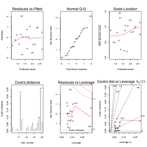
#goodness of fit
data.pois.resid <- sum(resid(data.pois.glm, type = "pearson")^2)
1 - pchisq(data.pois.resid, data.pois.glm$df.resid)
[1] 0.4897#Deviance based
1-pchisq(data.pois.glm$deviance, data.pois.glm$df.resid)[1] 0.5076data.pois.glmG <- glm(y~x, data=data.pois, family="gaussian")
library(MuMIn)
AICc(data.pois.glm, data.pois.glmG) df AICc
data.pois.glm 2 91.02
data.pois.glmG 3 99.78#Poisson deviance
data.pois.glm$deviance[1] 17.23#Gaussian deviance
data.pois.glmG$deviance[1] 118.1data.pois.resid/data.pois.glm$df.resid[1] 0.9717data.pois.glm$deviance/data.pois.glm$df.resid[1] 0.957#Or alternatively, via Pearson's residuals
Resid <- resid(data.pois.glm, type = "pearson")
sum(Resid^2) / (nrow(data.pois) - length(coef(data.pois.glm)))[1] 0.9717summary(data.pois.glm)
Call:
glm(formula = y ~ x, family = poisson(link = "log"), data = data.pois)

Deviance Residuals:
   Min      1Q  Median      3Q     Max
-1.635  -0.705   0.044   0.562   2.046

Coefficients:
            Estimate Std. Error z value Pr(>|z|)
(Intercept)   0.5600     0.2539    2.21    0.027
x             0.1115     0.0186    6.00    2e-09

(Intercept) *
x           ***
---
Signif. codes:
0 '***' 0.001 '**' 0.01 '*' 0.05 '.' 0.1 ' ' 1

(Dispersion parameter for poisson family taken to be 1)

    Null deviance: 55.614  on 19  degrees of freedom
Residual deviance: 17.226  on 18  degrees of freedom
AIC: 90.32

Number of Fisher Scoring iterations: 4library(gmodels)
ci(data.pois.glm) Estimate CI lower CI upper Std. Error
(Intercept) 0.5600 0.02649 1.0935 0.25395
x 0.1115 0.07247 0.1506 0.01858
p-value
(Intercept) 2.744e-02
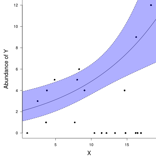
x 1.971e-091-(data.pois.glm$deviance/data.pois.glm$null)[1] 0.6903par(mfrow=c(1,1), mar = c(4, 5, 0, 0))
plot(y ~ x, data = data.pois, type = "n", ann = F, axes = F)
points(y ~ x, data = data.pois, pch = 16)
xs <- seq(min(data.pois$x), max(data.pois$x), len = 1000)
#ys <- predict(data.pois.glm, newdata = data.frame(x = xs), type = "response", se = T)
ys <- predict(data.pois.glm, newdata = data.frame(x = xs), type = "link", se = T)
ys$lwr <- exp(ys$fit - 2*ys$se.fit)
ys$upr <- exp(ys$fit + 2*ys$se.fit)
ys$fit <- exp(ys$fit)
lines(ys$fit ~ xs, col = "black")
lines(ys$lwr ~ xs, col = "black", lty = 2)
lines(ys$upr ~ xs, col = "black", lty = 2)
polygon(c(xs,rev(xs)), c(ys$lwr,rev(ys$upr)), border=NA, col="#0000FF50")
#lines(ys$fit - 2 * ys$se.fit ~ xs, col = "black", type = "l", lty = 2)
#lines(ys$fit + 2 * ys$se.fit ~ xs, col = "black", type = "l", lty = 2)
axis(1)
mtext("X", 1, cex = 1.5, line = 3)
axis(2, las = 2)
mtext("Abundance of Y", 2, cex = 1.5, line = 3)
box(bty = "l")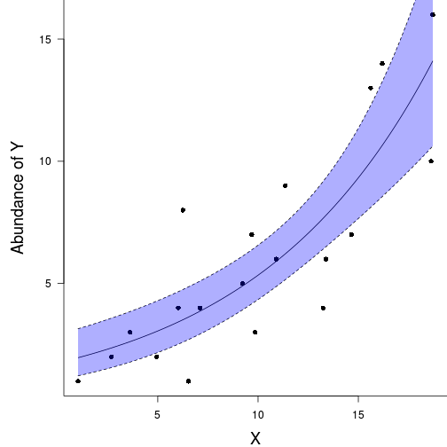
data.qp <- read.table('../data/data.qp.csv', header=T, sep=',', strip.white=T)
head(data.qp)
y x
1 0 1.025
2 3 2.697
3 0 3.626
4 5 4.949
5 6 6.025
6 1 6.254ggplot(data.qp, aes(y=y, x=x))+geom_point()+geom_rug()+
geom_smooth(method='lm')Error: could not find function "ggplot"## library(car)
## scatterplot(y~x,data=data.qp)
## scatterplot(y~x,data=data.qp, log='y')
plot(y~x, data.qp)
with(data.qp, lines(lowess(y~x)))
rug(jitter(data.qp$y), side=2)
plot(y~x, data.qp, log="y")
with(data.qp, lines(lowess(y~x)))
rug(jitter(data.qp$y), side=2)
hist(data.qp$y)
boxplot(data.qp$y, horizontal=TRUE)
rug(jitter(data.qp$y), side=1)
#Zero inflation
#proportion of 0's in the data
data.qp.tab<-table(data.qp$y==0)
data.qp.tab/sum(data.qp.tab)
FALSE  TRUE
 0.85  0.15
#proportion of 0's expected from a Poisson distribution
mu <- mean(data.qp$y)
cnts <- rpois(1000, mu)
data.qp.tab <- table(cnts == 0)
data.qp.tab/sum(data.qp.tab)
FALSE
    1
#fit model
data.qp.glm<-glm(y~x, data=data.qp, family="poisson")
data.qp.glm2 <- glm(y~x, data=data.qp, family="quasipoisson")
AICc(data.qp.glm, data.qp.glm2) df AICc
data.qp.glm 2 135.6
data.qp.glm2 2 NAanova(data.qp.glm, data.qp.glm2, test='Chisq')Analysis of Deviance Table
Model 1: y ~ x
Model 2: y ~ x
Resid. Df Resid. Dev Df Deviance Pr(>Chi)
1 18 70
2 18 70 0 0 #Model validation
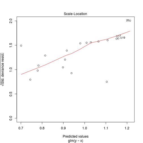
par(mfrow=c(2,3))
plot(data.qp.glm, ask=F, which=1:6)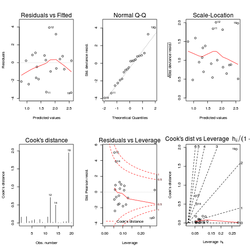
data.qp.glm$deviance/data.qp.glm$df.resid[1] 3.888#Or alternatively, via Pearson's residuals
Resid <- resid(data.qp.glm, type = "pearson")
sum(Resid^2) / (nrow(data.qp) - length(coef(data.qp.glm)))[1] 3.699summary(data.qp.glm)
Call:
glm(formula = y ~ x, family = "poisson", data = data.qp)

Deviance Residuals:
   Min      1Q  Median      3Q     Max
-3.366  -1.736  -0.124   0.744   3.933

Coefficients:
            Estimate Std. Error z value Pr(>|z|)
(Intercept)   0.6997     0.2468    2.84   0.0046
x             0.1005     0.0184    5.47  4.4e-08

(Intercept) **
x           ***
---
Signif. codes:
0 '***' 0.001 '**' 0.01 '*' 0.05 '.' 0.1 ' ' 1

(Dispersion parameter for poisson family taken to be 1)

    Null deviance: 101.521  on 19  degrees of freedom
Residual deviance:  69.987  on 18  degrees of freedom
AIC: 134.9

Number of Fisher Scoring iterations: 5library(gmodels)
ci(data.qp.glm) Estimate CI lower CI upper Std. Error
(Intercept) 0.6997 0.18121 1.218 0.24677
x 0.1005 0.06192 0.139 0.01835
p-value
(Intercept) 4.579e-03
x 4.389e-081-(data.qp.glm$deviance/data.qp.glm$null)[1] 0.3106par(mar = c(4, 5, 0, 0))
plot(y ~ x, data = data.qp, type = "n", ann = F, axes = F)
points(y ~ x, data = data.qp, pch = 16)
xs <- seq(0, 20, l = 1000)
ys <- predict(data.pois.glm, newdata = data.frame(x = xs), type = "link", se = T)
ys$lwr <- exp(ys$fit - 2*ys$se.fit)
ys$upr <- exp(ys$fit + 2*ys$se.fit)
ys$fit <- exp(ys$fit)
lines(ys$fit ~ xs, col = "black")
lines(ys$lwr ~ xs, col = "black", lty = 2)
lines(ys$upr ~ xs, col = "black", lty = 2)
axis(1)
mtext("X", 1, cex = 1.5, line = 3)
axis(2, las = 2)
mtext("Abundance of Y", 2, cex = 1.5, line = 3)
box(bty = "l")
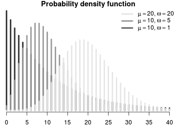
\[p(y_i)=\frac{\Gamma(y_i+\omega)}{\Gamma(\omega)y!}\times\frac{\mu_i^{y_i}\omega^\omega}{(\mu_i+\omega)^{\mu_i+\omega}}\]
data.nb <- read.table('../data/data.nb.csv', header=T, sep=',', strip.white=T)
head(data.nb)
y x
1 1 1.042
2 7 2.498
3 2 3.677
4 4 3.798
5 1 4.871
6 9 7.690scatterplot(y~x, data.nb, log='y')Error: NA/NaN/Inf in 'y'
plot(y~x, data.nb)
with(data.nb, lines(lowess(y~x)))
plot(y~x, data.nb, log="y")
with(data.nb, lines(lowess(y~x)))
rug(jitter(data.nb$y), side=2)
hist(data.nb$y, br=10)
boxplot(data.nb$y, horizontal=TRUE)
rug(jitter(data.nb$y), side=1)
#Zero inflation
#proportion of 0's in the data
data.nb.tab<-table(data.nb$y==0)
data.nb.tab/sum(data.nb.tab)
FALSE  TRUE
 0.95  0.05
#proportion of 0's expected from a Poisson distribution
mu <- mean(data.nb$y)
cnts <- rpois(1000, mu)
hist(cnts)
tab <- table(cnts == 0)
tab/sum(tab)
FALSE  TRUE
0.999 0.001
#fit model
library(MASS)
data.nb.glm <- glm.nb(y~x, data=data.nb)
#Model validation
par(mfrow=c(2,3))
plot(data.nb.glm, ask=F,which=1:6)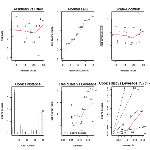
data.ss <- sum(resid(data.nb1, type = "pearson")^2)Error: object 'data.nb1' not founddata.ss/data.nb1$df.residError: object 'data.ss' not founddata.nb1 <- glm(y~x, data=data.nb, family='poisson')
plot(data.nb1, ask=F,which=1:6)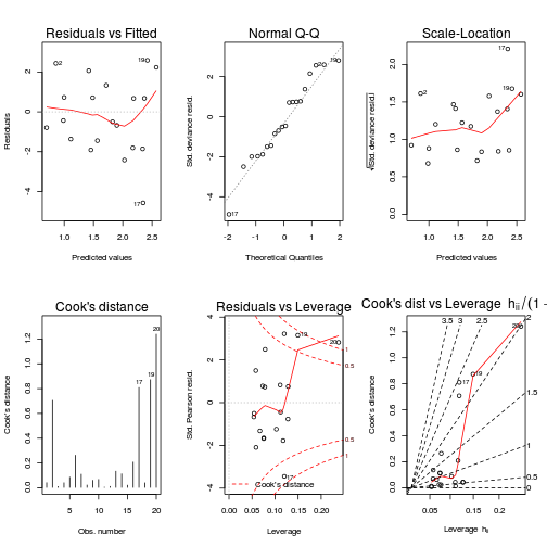
1-pchisq(data.nb1$deviance, data.nb1$df.resid)[1] 8.6e-08#goodness of fit
data.nb.resid <- sum(resid(data.nb.glm, type = "pearson")^2)
1 - pchisq(data.nb.resid, data.nb.glm$df.resid)[1] 0.5825#Deviance based
1-pchisq(data.nb.glm$deviance, data.nb.glm$df.resid)[1] 0.2407data.nb.glmG <- glm(y~x, data=data.nb, family="gaussian")
AIC(data.nb.glm, data.nb.glmG) df AIC
data.nb.glm 3 115.8
data.nb.glmG 3 128.2#Poisson deviance
data.nb.glm$deviance[1] 21.81#Gaussian deviance
data.nb.glmG$deviance[1] 527.6summary(data.nb.glm)
Call:
glm.nb(formula = y ~ x, data = data.nb, init.theta = 2.359878187,
    link = log)

Deviance Residuals:
   Min      1Q  Median      3Q     Max
-2.787  -0.894  -0.317   0.442   1.366

Coefficients:
            Estimate Std. Error z value Pr(>|z|)
(Intercept)   0.7454     0.4253    1.75   0.0797
x             0.0949     0.0344    2.76   0.0058

(Intercept) .
x           **
---
Signif. codes:
0 '***' 0.001 '**' 0.01 '*' 0.05 '.' 0.1 ' ' 1

(Dispersion parameter for Negative Binomial(2.36) family taken to be 1)

    Null deviance: 30.443  on 19  degrees of freedom
Residual deviance: 21.806  on 18  degrees of freedom
AIC: 115.8

Number of Fisher Scoring iterations: 1

              Theta:  2.36
          Std. Err.:  1.10

2 x log-likelihood: -109.85 library(gmodels)
ci(data.nb.glm) Estimate CI lower CI upper Std. Error
(Intercept) 0.74543 -0.14818 1.6390 0.42534
x 0.09494 0.02265 0.1672 0.03441
p-value
(Intercept) 0.079682
x 0.0057921-(data.nb.glm$deviance/data.nb.glm$null)[1] 0.2837par(mfrow=c(1,1),mar = c(4, 5, 0, 0))
plot(y ~ x, data = data.nb, type = "n", ann = F, axes = F)
points(y ~ x, data = data.nb, pch = 16)
xs <- seq(0, 20, l = 1000)
ys <- predict(data.nb.glm, newdata = data.frame(x = xs), type = "link", se = T)
ys$lwr <- exp(ys$fit - 2*ys$se.fit)
ys$upr <- exp(ys$fit + 2*ys$se.fit)
ys$fit <- exp(ys$fit)
lines(ys$fit ~ xs, col = "black")
lines(ys$lwr ~ xs, col = "black", lty = 2)
lines(ys$upr ~ xs, col = "black", lty = 2)
axis(1)
mtext("X", 1, cex = 1.5, line = 3)
axis(2, las = 2)
mtext("Abundance of Y", 2, cex = 1.5, line = 3)
box(bty = "l")
data.zip <- read.csv('../data/data.zip.csv', strip.white=T)
head(data.zip)
y x
1 0 1.042
2 3 2.498
3 1 3.677
4 4 3.798
5 5 4.871
6 1 7.690ggplot(data.zip, aes(y=y, x=x))+geom_point()Error: could not find function "ggplot"plot(y~x, data.zip)
with(data.zip, lines(lowess(y~x)))
plot(y~x, data.zip, log="y")
with(data.zip, lines(lowess(y~x)))
rug(jitter(data.pois$y), side=2)
hist(data.zip$y, br=20)
boxplot(data.zip$y, horizontal=TRUE)
rug(jitter(data.zip$y), side=1)
#Zero inflation
#proportion of 0's in the data
data.zip.tab<-table(data.zip$y==0)
data.zip.tab/sum(data.zip.tab)
FALSE  TRUE
 0.55  0.45
#proportion of 0's expected from a Poisson distribution
mu <- mean(data.zip$y)
cnts <- rpois(1000, mu)
data.zip.tab <- table(cnts == 0)
data.zip.tab/sum(data.zip.tab)
FALSE  TRUE
0.929 0.071 summary(glm(y~x, data.zip, family="poisson"))
Call:
glm(formula = y ~ x, family = "poisson", data = data.zip)

Deviance Residuals:
   Min      1Q  Median      3Q     Max
-2.541  -2.377  -0.975   1.174   3.638

Coefficients:
            Estimate Std. Error z value Pr(>|z|)
(Intercept)   0.6705     0.3302    2.03    0.042
x             0.0296     0.0266    1.11    0.266

(Intercept) *
x
---
Signif. codes:
0 '***' 0.001 '**' 0.01 '*' 0.05 '.' 0.1 ' ' 1

(Dispersion parameter for poisson family taken to be 1)

    Null deviance: 85.469  on 19  degrees of freedom
Residual deviance: 84.209  on 18  degrees of freedom
AIC: 124

Number of Fisher Scoring iterations: 6plot(glm(y~x, data.zip, family="poisson"))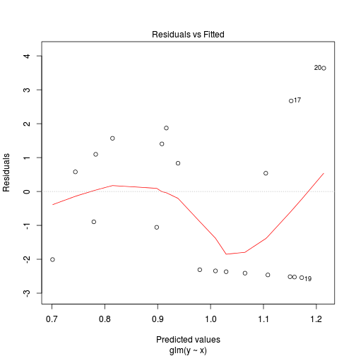

library(pscl)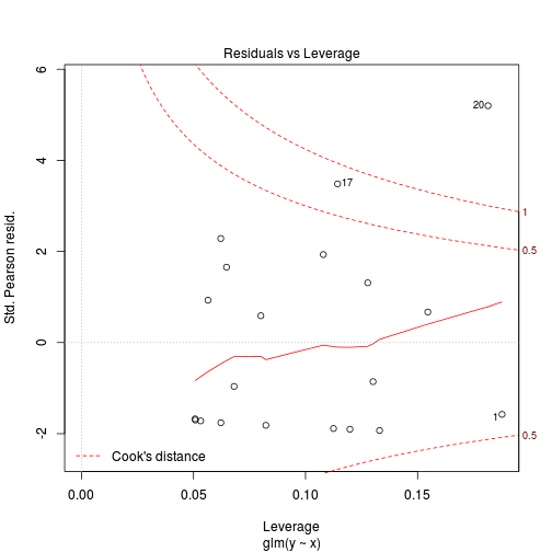
data.zip.zip <- zeroinfl(y ~ x | 1, dist = "poisson", data = data.zip)
plot(resid(data.zip.zip)~fitted(data.zip.zip))
summary(data.zip.zip)
Call:
zeroinfl(formula = y ~ x | 1, data = data.zip,
    dist = "poisson")

Pearson residuals:
   Min     1Q Median     3Q    Max
-1.001 -0.956 -0.393  0.966  1.619

Count model coefficients (poisson with log link):
            Estimate Std. Error z value Pr(>|z|)
(Intercept)   0.7047     0.3196    2.21  0.02745
x             0.0873     0.0253    3.45  0.00056

(Intercept) *
x           ***

Zero-inflation model coefficients (binomial with logit link):
            Estimate Std. Error z value Pr(>|z|)
(Intercept)   -0.229      0.456    -0.5     0.62
---
Signif. codes:  0 '***' 0.001 '**' 0.01 '*' 0.05 '.' 0.1 ' ' 1

Number of iterations in BFGS optimization: 13
Log-likelihood: -36.2 on 3 Df
data.zip.zip1 <- zeroinfl(y ~ x | x, dist = "poisson", data = data.zip)
plot(resid(data.zip.zip1)~fitted(data.zip.zip1))
summary(data.zip.zip1)
Call:
zeroinfl(formula = y ~ x | x, data = data.zip,
    dist = "poisson")

Pearson residuals:
   Min     1Q Median     3Q    Max
-1.276 -0.781 -0.593  0.908  2.132

Count model coefficients (poisson with log link):
            Estimate Std. Error z value Pr(>|z|)
(Intercept)   0.6111     0.3300    1.85  0.06404
x             0.0939     0.0257    3.65  0.00027

(Intercept) .
x           ***

Zero-inflation model coefficients (binomial with logit link):
            Estimate Std. Error z value Pr(>|z|)
(Intercept)   -2.731      1.890   -1.44     0.15
x              0.217      0.146    1.49     0.14
---
Signif. codes:  0 '***' 0.001 '**' 0.01 '*' 0.05 '.' 0.1 ' ' 1

Number of iterations in BFGS optimization: 17
Log-likelihood: -34.4 on 4 DfAIC(data.zip.zip, data.zip.zip1) df AIC
data.zip.zip 3 78.34
data.zip.zip1 4 76.81par(mar = c(4, 5, 0, 0))
plot(y ~ x, data = data.zip, type = "n", ann = F, axes = F)
points(y ~ x, data = data.zip, pch = 16)
xs <- seq(0, 20, l = 1000)
#ys <- predict(data.pois.glm, newdata = data.frame(x = xs), type = "response", se = T)
coefs <- coef(data.zip.zip)[1:2]
mm <- model.matrix(~x, data=data.frame(x=xs))
fit <- coefs %*% t(mm)
se <- sqrt(diag(mm %*% vcov(data.zip.zip)[-3,-3] %*% t(mm)))
lwr <- as.vector(exp(fit - 2*se))
upr <- as.vector(exp(fit + 2*se))
fit <- as.vector(exp(fit))
lines(fit ~ xs, col = "black")
lines(lwr ~ xs, col = "black", lty = 2)
lines(upr ~ xs, col = "black", lty = 2)
polygon(c(xs,rev(xs)), c(lwr,rev(upr)), border=NA, col="#0000FF50")
#lines(ys$fit - 2 * ys$se.fit ~ xs, col = "black", type = "l", lty = 2)
#lines(ys$fit + 2 * ys$se.fit ~ xs, col = "black", type = "l", lty = 2)
axis(1)
mtext("X", 1, cex = 1.5, line = 3)
axis(2, las = 2)
mtext("Abundance of Y", 2, cex = 1.5, line = 3)
box(bty = "l")