Limitations of Linear Models

Feature complexity
- non-linear trends (GAM)
- complex (multi-way) interactions
- non-additive interactions

Limitations of Linear Models

Feature complexity
- non-linear trends (GAM)
- complex (multi-way) interactions
- non-additive interactions

single models fail to capture complexity

Limitations of Linear Models

Feature complexity
Prediction
Relative importance
(Multi)collinearity

Classication & Regression Trees

Advantanges

Feature complexity
Prediction
Relative importance
(Multi)collinearity

Classication & Regression Trees

Diss-advantanges

over-fitting (over learning)

Classication & Regression Trees

Classification

Categorical response

Regression

Continuous response

CART

Simple regression trees

split (partition) data up into major chunks

Simple regression trees

split (partition) data up into major chunks
- maximizing change in explained deviance
- when Gaussian error,
  - maximizing between group SS
  - minimizing SSerror

Simple regression trees

split (partition) data up into major chunks

Simple regression trees

split (partition) data up into major chunks

Simple regression trees

split (partition) data up into major chunks

Simple regression trees

split these subsets

Simple regression trees

split these subsets

Simple regression trees

split these subsets

Simple regression trees

split these subsets

Simple regression trees

recursively partition (split)
decision tree
simple trees tend to overfit.
- error is fitted along with the model

Simple regression trees

Pruning

reduce overfitting
- deviance at each terminal node (leaf)

Simple regression trees

Predictions

partial plots

Classification and Regression Trees

R packages

simple CART

library(tree)

an extension that facilitates (some) non-gaussian errors

library(rpart)

Classification and Regression Trees

Limitations

crude overfitting protection
low resolution
limited error distributions
little scope for random effects

Boosted regression Trees

Boosting

machine learning meets predictive modelling
ensemble models
- sequence of simple Trees (10,000+ trees)
- built to predict residuals of previous tree
- shrinkage
- produce excellent fit

Boosted regression Trees

Over fitting

over vs under fitting
residual error vs precision
minimizing square error loss

Boosted regression Trees

minimizing square error loss

test (validation) data
- 75% train, 25% test

out of bag
- 50% in, 50% out

cross validation
- 3 folds

Boosted regression Trees

Over fitting

Error: unused argument (to = c(0.5, 2.5))

Error: unused argument (to = c(0, 1))

Error: object 'at' not found

Boosted regression Trees

Predictions

Boosted regression Trees

Variable importance

   var rel.inf
x1  x1   55.06
x2  x2   44.94

Boosted regression Trees

\(R^2\)

[1] 0.5952

Worked Examples

paruelo <- read.table('../data/paruelo.csv', header=T, sep=',', strip.white=T)
head(paruelo)

    C3   LAT   LONG MAP  MAT JJAMAP DJFMAP
1 0.65 46.40 119.55 199 12.4   0.12   0.45
2 0.65 47.32 114.27 469  7.5   0.24   0.29
3 0.76 45.78 110.78 536  7.2   0.24   0.20
4 0.75 43.95 101.87 476  8.2   0.35   0.15
5 0.33 46.90 102.82 484  4.8   0.40   0.14
6 0.03 38.87  99.38 623 12.0   0.40   0.11

library(tree)
paruelo.tree <- tree(C3 ~ LAT+LONG+MAP+MAT+JJAMAP,
       data=paruelo)
plot(residuals(paruelo.tree)~predict(paruelo.tree))

plot(paruelo.tree)
text(paruelo.tree, cex=0.75)

plot(prune.tree(paruelo.tree))

paruelo.tree1 <- prune.tree(paruelo.tree, best=4)
plot(residuals(paruelo.tree1)~predict(paruelo.tree1))

plot(paruelo.tree1)
text(paruelo.tree1)

summary(paruelo.tree1)


Regression tree:
snip.tree(tree = paruelo.tree, nodes = c(7L, 5L, 4L, 6L))
Variables actually used in tree construction:
[1] "LAT" "MAT"
Number of terminal nodes:  4 
Residual mean deviance:  0.0304 = 2.1 / 69 
Distribution of residuals:
   Min. 1st Qu.  Median    Mean 3rd Qu.    Max. 
-0.4220 -0.1010 -0.0325  0.0000  0.0787  0.4820

paruelo.tree1$frame

     var  n    dev   yval splits.cutleft
1    LAT 73 4.9093 0.2714        <42.785
2    MAT 50 1.6364 0.1592          <7.25
4 <leaf> 12 0.4384 0.3425               
5 <leaf> 38 0.6674 0.1013               
3    MAT 23 1.2762 0.5152           <6.9
6 <leaf> 12 0.6912 0.4083               
7 <leaf> 11 0.2984 0.6318               
  splits.cutright
1         >42.785
2           >7.25
4                
5                
3            >6.9
6                
7

library(scales)

#ys <- with(paruelo,
#rescale(C3, from=c(min(C3), max(C3)),
#to=c(0.8,0)))
#plot(paruelo$LONG,paruelo$LAT,col=grey(ys),
#pch=20,xlab="Longitude",ylab="Latitude")
#partition.tree(paruelo.tree1,ordvars=c("MAT","LAT"),add=TRUE)
#partition.tree(paruelo.tree1,add=TRUE)

#Prediction
xlat <- seq(min(paruelo$LAT), max(paruelo$LAT), l=100)
#xlong <- mean(paruelo$LONG)
#xmat <- mean(paruelo$MAT)
pred <- predict(paruelo.tree1,
    newdata=data.frame(LAT=xlat, LONG=mean(paruelo$LONG), MAT=mean(paruelo$MAT),
      MAP=mean(paruelo$MAP),
      JJAMAP=mean(paruelo$JJAMAP)))
par(mfrow=c(1,2))
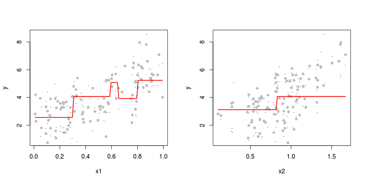
plot(C3~LAT, paruelo, type="p",pch=16, cex=0.2)
points(I(predict(paruelo.tree1)-resid(paruelo.tree1))
~LAT, paruelo, type="p",pch=16, col="grey")
lines(pred~xlat, col="red", lwd=2)

xmat <- seq(min(paruelo$MAT), max(paruelo$MAT), l=100)
#xlat <- mean(paruelo$LAT)
pred <- predict(paruelo.tree1,
    newdata=data.frame(LAT=mean(paruelo$LAT), LONG=mean(paruelo$LONG), MAT=xmat,
      MAP=mean(paruelo$MAP),
      JJAMAP=mean(paruelo$JJAMAP)))
plot(C3~MAT, paruelo, type="p",pch=16, cex=0.2)
points(I(predict(paruelo.tree1)-resid(paruelo.tree1))~MAT, paruelo, type="p",pch=16, col="grey")
lines(pred~xmat, col="red", lwd=2)

#xlong <- seq(min(paruelo$LONG), max(paruelo$LONG), l=100)
##xlat <- mean(paruelo$LAT)
#pred <- predict(paruelo.tree1,
#    newdata=data.frame(LAT=mean(paruelo$LAT), LONG=xlong, MAT=mean(paruelo$MAT),
#      MAP=mean(paruelo$MAP),
#      JJAMAP=mean(paruelo$JJAMAP)))
#plot(C3~LONG, paruelo, type="p",pch=16, cex=0.2)
#points(I(predict(paruelo.tree1)-resid(paruelo.tree1))~LONG, paruelo, type="p",pch=16, col="grey")
#lines(pred~xlong, col="red", lwd=2)


## paruelo.tree <- tree(C3 ~ LAT+LONG+MAP+MAT+
## JJAMAP+DJFMAP, data=paruelo)
## plot(paruelo.tree)
## text(paruelo.tree, cex=0.75)

## xlat <- seq(min(paruelo$LAT), max(paruelo$LAT), l=100)
## xlong <- mean(paruelo$LONG)
## xmat<- mean(paruelo$MAT)
## xmap<- mean(paruelo$MAP)
## xjjamap<- mean(paruelo$JJAMAP)
## xdjfmap<- mean(paruelo$DJFMAP)

## pp <- predict(paruelo.tree1, newdata=data.frame(LAT=xlat, LONG=xlong, MAT=xmat, MAP=xmap, JJAMAP=xjjamap, DJFMAP=xdjfmap))
## par(mfrow=c(1,2))
## plot(C3~LAT, paruelo, type="p",pch=16, cex=0.2)
## points(I(predict(paruelo.tree1)-resid(paruelo.tree1))~LAT, paruelo, type="p",pch=16, col="grey")
## lines(pp~xlat, col="red", lwd=2)


## xlat <- mean(paruelo$LAT)
## xlong <- mean(paruelo$LONG)
## xmat<- seq(min(paruelo$MAT), max(paruelo$MAT), l=100)
## xmap<- mean(paruelo$MAP)
## xjjamap<- mean(paruelo$JJAMAP)
## xdjfmap<- mean(paruelo$DJFMAP)

## pp <- predict(paruelo.tree1, newdata=data.frame(LAT=xlat, LONG=xlong, MAT=xmat, MAP=xmap, JJAMAP=xjjamap, DJFMAP=xdjfmap))
## par(mfrow=c(1,2))
## plot(C3~MAT, paruelo, type="p",pch=16, cex=0.2)
## points(I(predict(paruelo.tree1)-resid(paruelo.tree1))~MAT, paruelo, type="p",pch=16, col="grey")
## lines(pp~xmat, col="red", lwd=2)



## Now GBM
library(gbm)
paruelo.gbm <- gbm(C3~LAT+LONG+MAP+MAT+JJAMAP+DJFMAP,
   data=paruelo,
   distribution="gaussian",
   n.trees=10000,
   interaction.depth=3, # 1: additive model, 2: two-way interactions, etc.
   cv.folds=3,
   train.fraction=0.75,
   bag.fraction=0.5,
   shrinkage=0.001,
   n.minobsinnode=2)

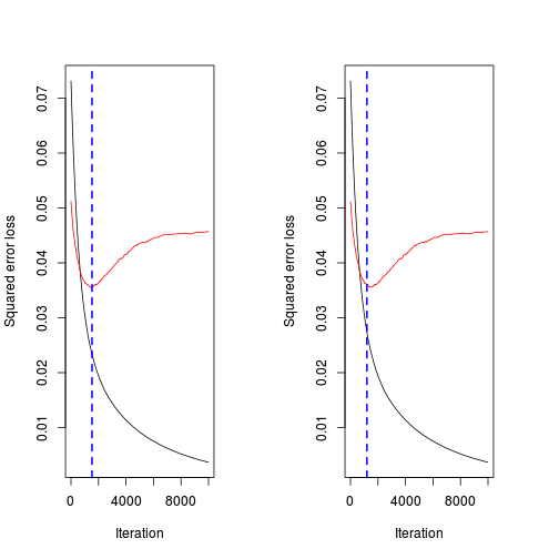
## Out of Bag method of determining number of iterations
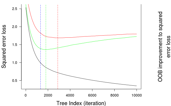
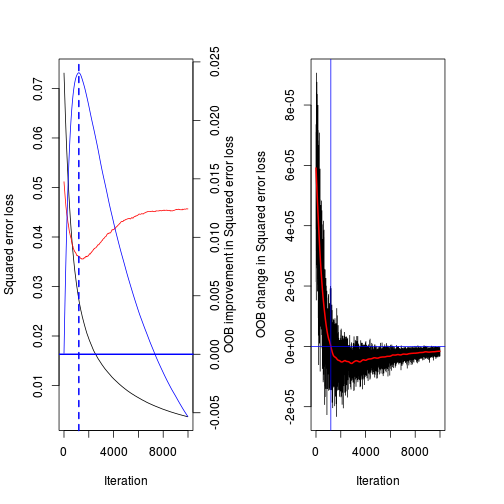
(best.iter <- gbm.perf(paruelo.gbm, method="test"))

[1] 1533

(best.iter <- gbm.perf(paruelo.gbm, method="OOB"))

[1] 1197

(best.iter <- gbm.perf(paruelo.gbm, method="OOB",oobag.curve=TRUE,overlay=TRUE, plot.it=TRUE))

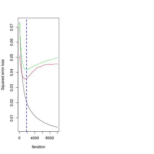
[1] 1197

(best.iter <- gbm.perf(paruelo.gbm, method="cv"))

[1] 1844

par(mfrow=c(1,2))

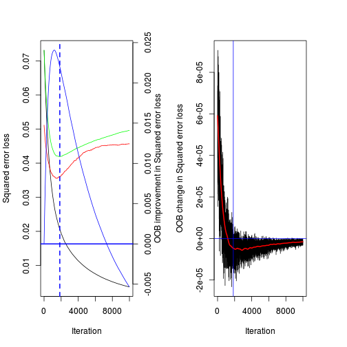
best.iter <- gbm.perf(paruelo.gbm, method="cv",
   oobag.curve=TRUE,overlay=TRUE,plot.it=TRUE)

best.iter

[1] 1844

par(mfrow=c(3,2),mar=c(4,5,0,0))
plot(paruelo.gbm, 1, n.tree=best.iter)
plot(paruelo.gbm, 2, n.tree=best.iter)
plot(paruelo.gbm, 3, n.tree=best.iter)
plot(paruelo.gbm, 4, n.tree=best.iter)
plot(paruelo.gbm, 5, n.tree=best.iter)
plot(paruelo.gbm, 6, n.tree=best.iter)

par(mfrow=c(3,2),mar=c(4,5,0,0))
plot(paruelo.gbm, 1, n.tree=best.iter, ylim=c(0.1,0.6))
plot(paruelo.gbm, 2, n.tree=best.iter, ylim=c(0.1,0.6))
plot(paruelo.gbm, 3, n.tree=best.iter, ylim=c(0.1,0.6))
plot(paruelo.gbm, 4, n.tree=best.iter, ylim=c(0.1,0.6))
plot(paruelo.gbm, 5, n.tree=best.iter, ylim=c(0.1,0.6))
plot(paruelo.gbm, 6, n.tree=best.iter, ylim=c(0.1,0.6))

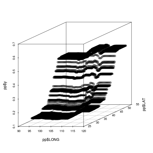
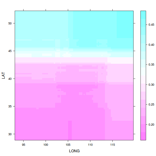
pp<-plot(paruelo.gbm, c(2,1), best.iter,
         return.grid=TRUE)

#scatter3d(x=pp$LONG, y=pp$LAT, z=pp$y)
par(mfrow=c(1,1))
library(scatterplot3d)
scatterplot3d(x=pp$LONG, y=pp$LAT, z=pp$y, angle=24)

#with(pp[1:20,],persp(x=LONG, y=LAT, z=y))
xyz <- with(pp,unique(cbind(x=LONG,y=LAT,z=pp$y)))
persp(xyz, theta=-60, phi=-10)

par(mfrow=c(1,1))
summary(paruelo.gbm)

          var rel.inf
LAT       LAT  41.736
LONG     LONG  14.058
MAT       MAT  14.057
MAP       MAP  13.052
DJFMAP DJFMAP   8.827
JJAMAP JJAMAP   8.270

## interact.gbm’ computes Friedman's H-statistic to assess the
##      relative strength of interaction effects in non-linear models. H
##      is on the scale of [0-1] with higher values indicating larger
##      interaction effects. To connect to a more familiar measure, if x_1
##      and x_2 are uncorrelated covariates with mean 0 and variance 1 and
##      the model is of the form

##                    y=beta_0+beta_1x_1+beta_2x_2+beta_3x_3               
     
##      then

##               H=\frac{beta_3}{sqrt{beta_1^2+beta_2^2+beta_3^2}}         
     
##      Note that if the main effects are weak, the estimated H will be
##      unstable. For example, if (in the case of a two-way interaction)
##      neither main effect is in the selected model (relative influence
##      is zero), the result will be 0/0. Also, with weak main effects,
##      rounding errors can result in values of H > 1 which are not
##      possible.

interact.gbm(paruelo.gbm, paruelo,1:2,n.tree=best.iter)

[1] 0.06536

interact.gbm(paruelo.gbm, paruelo,c(1,3),n.tree=best.iter)

[1] 0.0537

interact.gbm(paruelo.gbm, paruelo,c(1,2,3),n.tree=best.iter)

[1] 0.002928

## terms <- attr(paruelo.gbm$Terms,"term.labels")
## for (i in 1:5) {
##  for (j in (i+1):6) {
##    print(paste(terms[i],":",terms[j],"=",
##           interact.gbm(paruelo.gbm, paruelo,c(i,j),n.tree=best.iter),sep=""))
##  }
## }

terms <- attr(paruelo.gbm$Terms,"term.labels")
paruelo.int <- NULL
for (i in 1:(length(terms)-1)) {
 for (j in (i+1):length(terms)) {
   paruelo.int <- rbind(paruelo.int,
        data.frame(Var1=terms[i], Var2=terms[j],
  "H.stat"=interact.gbm(paruelo.gbm, paruelo,c(i,j),
   n.tree=best.iter)
                   ))
 }
}
paruelo.int

     Var1   Var2  H.stat
1     LAT   LONG 0.06536
2     LAT    MAP 0.05370
3     LAT    MAT 0.09307
4     LAT JJAMAP 0.04462
5     LAT DJFMAP 0.04217
6    LONG    MAP 0.04100
7    LONG    MAT 0.03779
8    LONG JJAMAP 0.02226
9    LONG DJFMAP 0.09464
10    MAP    MAT 0.09162
11    MAP JJAMAP 0.02688
12    MAP DJFMAP 0.01857
13    MAT JJAMAP 0.14502
14    MAT DJFMAP 0.15350
15 JJAMAP DJFMAP 0.08397

plot(paruelo.gbm, c(2,1), n.tree=best.iter)

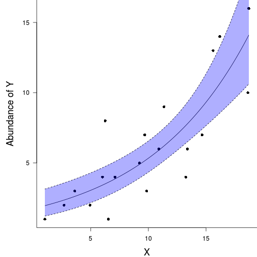
loyn <- read.table('../data/loyn.csv', header=T, sep=',', strip.white=T)
head(loyn)

  ABUND AREA YR.ISOL DIST LDIST GRAZE ALT
1   5.3  0.1    1968   39    39     2 160
2   2.0  0.5    1920  234   234     5  60
3   1.5  0.5    1900  104   311     5 140
4  17.1  1.0    1966   66    66     3 160
5  13.8  1.0    1918  246   246     5 140
6  14.1  1.0    1965  234   285     3 130

loyn$fGRAZE<- factor(loyn$GRAZE)
head(loyn)

  ABUND AREA YR.ISOL DIST LDIST GRAZE ALT fGRAZE
1   5.3  0.1    1968   39    39     2 160      2
2   2.0  0.5    1920  234   234     5  60      5
3   1.5  0.5    1900  104   311     5 140      5
4  17.1  1.0    1966   66    66     3 160      3
5  13.8  1.0    1918  246   246     5 140      5
6  14.1  1.0    1965  234   285     3 130      3

library(tree)
loyn.tree <- tree(ABUND~AREA+YR.ISOL+DIST+
   LDIST+fGRAZE+ALT, data=loyn, mindev=0)
plot(residuals(loyn.tree)~predict(loyn.tree))

plot(loyn.tree, type="uniform")
text(loyn.tree,cex=1, all=T)
text(loyn.tree,lab=paste("n"),
    cex=1,adj=c(0,2), splits=F)

plot(prune.tree(loyn.tree))

loyn.tree.prune<-prune.tree(loyn.tree,
    best=3)
plot(loyn.tree.prune, type="uniform")
text(loyn.tree.prune,cex=1, all=T)
text(loyn.tree.prune,lab=paste("n"),
     cex=1,adj=c(0,2), splits=F)

library(rpart)
loyn.rpart<-rpart(ABUND~AREA+YR.ISOL+
  DIST+LDIST+GRAZE+ALT, data=loyn)
plot(loyn.rpart)
text(loyn.rpart,use.n=TRUE)

#gbm
library(gbm)
loyn.gbm <- gbm(ABUND~DIST+LDIST+AREA+
                fGRAZE+ALT+YR.ISOL,
                data=loyn,
                distribution="gaussian",
                train=1,
                interaction.depth=3,
                cv.folds=1,
                shrinkage=0.001,
                bag.fraction=0.5,
                n.minobsinnode=2,
                n.trees=10000)

Error: object 'p' not found

#loyn.gbm <- gbm(C3~LAT + LONG + MAP + MAT + JJAMAP + DJFMAP, data=loyn,
#                   interaction.depth=3, cv.folds=3, dist="bernoulli")

#best.iter <- gbm.perf(loyn.gbm, method="test") #see graph
#best.iter <- gbm.perf(loyn.gbm, method="OOB", plot.it=TRUE) #see graph

par(mfrow=c(1,2))
(best.iter <- gbm.perf(loyn.gbm, method="OOB",
                       overlay=TRUE,oobag.curve=TRUE))

Error: object 'loyn.gbm' not found

#print(best.iter)
summary(loyn.gbm,n.trees=best.iter) #see graph

Error: object 'loyn.gbm' not found

par(mfrow=c(2,3))
plot(loyn.gbm, 1, best.iter)

Error: object 'loyn.gbm' not found

plot(loyn.gbm, 2, best.iter)

Error: object 'loyn.gbm' not found

plot(loyn.gbm, 3, best.iter)

Error: object 'loyn.gbm' not found

plot(loyn.gbm, 4, best.iter)

Error: object 'loyn.gbm' not found

plot(loyn.gbm, 5, best.iter)

Error: object 'loyn.gbm' not found

plot(loyn.gbm, 6, best.iter)

Error: object 'loyn.gbm' not found

par(mfrow=c(2,3))
plot(loyn.gbm, 1, best.iter, ylim=c(10,30))

Error: object 'loyn.gbm' not found

plot(loyn.gbm, 2, best.iter, ylim=c(10,30))

Error: object 'loyn.gbm' not found

plot(loyn.gbm, 3, best.iter, ylim=c(10,30))

Error: object 'loyn.gbm' not found

plot(loyn.gbm, 4, best.iter, ylim=c(10,30))

Error: object 'loyn.gbm' not found

plot(loyn.gbm, 5, best.iter, ylim=c(10,30))

Error: object 'loyn.gbm' not found

plot(loyn.gbm, 6, best.iter, ylim=c(10,30))

Error: object 'loyn.gbm' not found

dists <- seq(min(loyn$DIST),max(loyn$DIST),l=100)
ldists <- seq(min(loyn$LDIST),max(loyn$LDIST),l=100)
areas <- seq(min(loyn$AREA),max(loyn$AREA),l=100)
grazes <- seq(min(loyn$GRAZE),max(loyn$GRAZE),l=100)
alts <- seq(min(loyn$ALT),max(loyn$ALT),l=100)
yrs <- seq(min(loyn$YR.ISOL),max(loyn$YR.ISOL),l=100)


new<-predict(loyn.gbm,
             newdata=data.frame(
               DIST=10,
               LDIST=10,
               AREA=500,
               fGRAZE=2,
               ALT=200,
               YR.ISOL=1960
               ), n.trees=best.iter
             )

Error: object 'loyn.gbm' not found

new

function (Class, ...) 
{
    ClassDef <- getClass(Class, where = topenv(parent.frame()))
    value <- .Call(C_new_object, ClassDef)
    initialize(value, ...)
}
<bytecode: 0x3239690>
<environment: namespace:methods>

#plot(aa~areas, type="l",ylim=c(7,30))

aa<-predict(loyn.gbm, newdata=data.frame(
                        DIST=800,
                       LDIST=800,
                       AREA=areas,
                       fGRAZE=1,
                       ALT=1000,
                       YR.ISOL=10
                       ), n.trees=best.iter
        )

Error: object 'loyn.gbm' not found

plot(aa~areas, type="l")

Error: object 'aa' not found

plot(aa~areas, type="l",log="x")

Error: object 'aa' not found

aa<-predict(loyn.gbm, newdata=data.frame(
                        DIST=mean(dists),
                       LDIST=mean(ldists),
                       AREA=areas,
                       GRAZE=mean(grazes),
                       ALT=200,
                       YR.ISOL=mean(yrs)
                       ), n.trees=best.iter
        )

Error: object 'loyn.gbm' not found

aa<-predict(loyn.gbm, newdata=data.frame(
                        DIST=mean(loyn$DIST),
                       LDIST=mean(loyn$LDIST),
                       AREA=mean(loyn$AREA),
                       GRAZE=grazes,
                       ALT=mean(loyn$ALT),
                       YR.ISOL=mean(loyn$YR.ISOL)
                       ), n.trees=best.iter
        )

Error: object 'loyn.gbm' not found

plot(aa~grazes, type="l")

Error: object 'aa' not found

terms <- attr(loyn.gbm$Terms,"term.labels")

Error: object 'loyn.gbm' not found

loyn.int <- NULL
for (i in 1:(length(terms)-1)) {
 for (j in (i+1):length(terms)) {
   loyn.int <- rbind(loyn.int,
        data.frame(Var1=terms[i], Var2=terms[j],
                   "H.stat"=interact.gbm(loyn.gbm, loyn,c(i,j),n.tree=best.iter)
                   ))
 }
}

Error: object 'loyn.gbm' not found

loyn.int

NULL

loyn.gbm <- gbm(ABUND~DIST+LDIST+AREA+
      factor(GRAZE)+ALT+YR.ISOL, data=loyn,
      interaction.depth=3, cv.folds=3,train=0.5,
      n.minobsinnode=2, n.trees=10000)

Distribution not specified, assuming gaussian ...

Error: subscript out of bounds

best.iter <- gbm.perf(loyn.gbm, method="cv") #see graph

Error: object 'loyn.gbm' not found

print(best.iter)

[1] 1844

summary(loyn.gbm,n.trees=best.iter) #see graph

Error: object 'loyn.gbm' not found

plot(loyn.gbm, 3:4, best.iter, ylim=c(10,30))

Error: object 'loyn.gbm' not found

##PARUELO
paruelo <- read.table('../data/paruelo.csv', header=T, sep=',', strip.white=T)
head(paruelo)

    C3   LAT   LONG MAP  MAT JJAMAP DJFMAP
1 0.65 46.40 119.55 199 12.4   0.12   0.45
2 0.65 47.32 114.27 469  7.5   0.24   0.29
3 0.76 45.78 110.78 536  7.2   0.24   0.20
4 0.75 43.95 101.87 476  8.2   0.35   0.15
5 0.33 46.90 102.82 484  4.8   0.40   0.14
6 0.03 38.87  99.38 623 12.0   0.40   0.11

## @knitr ws4-Q1-2
#via car's scatterplotMatrix function
library(car)
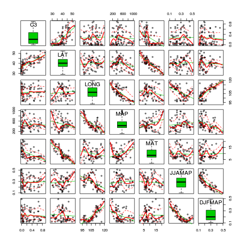
scatterplotMatrix(~C3+LAT+LONG+MAP+MAT+JJAMAP+DJFMAP, data=paruelo, diagonal='boxplot')

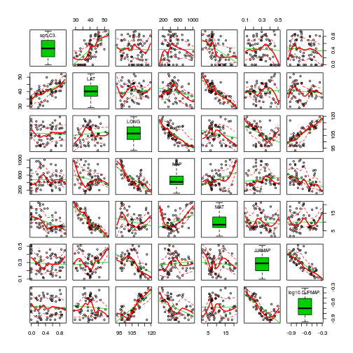
scatterplotMatrix(~sqrt(C3)+LAT+LONG+MAP+MAT+JJAMAP+log10(DJFMAP), data=paruelo, diagonal='boxplot')

library(car)
vif(lm(sqrt(paruelo$C3) ~ LAT + LONG + MAP + MAT + JJAMAP + DJFMAP, data=paruelo))

   LAT   LONG    MAP    MAT JJAMAP DJFMAP 
 3.503  5.268  2.799  3.743  3.163  5.710

library(car)
1/vif(lm(sqrt(paruelo$C3) ~ LAT + LONG + MAP + MAT + JJAMAP + log10(DJFMAP), data=paruelo))

          LAT          LONG           MAP 
       0.2809        0.2005        0.3579 
          MAT        JJAMAP log10(DJFMAP) 
       0.2665        0.3130        0.1829

paruelo$cLAT <- scale(paruelo$LAT, scale=F)
paruelo$cLONG <- scale(paruelo$LONG, scale=F)


## @knitr Q1-5
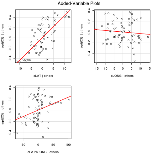
paruelo.lm <- lm(sqrt(C3) ~ cLAT*cLONG, data=paruelo)

summary(paruelo.lm)


Call:
lm(formula = sqrt(C3) ~ cLAT * cLONG, data = paruelo)

Residuals:
    Min      1Q  Median      3Q     Max 
-0.5131 -0.1343 -0.0113  0.1409  0.3894 

Coefficients:
             Estimate Std. Error t value Pr(>|t|)
(Intercept)  0.428266   0.023435   18.27  < 2e-16
cLAT         0.043694   0.004867    8.98  3.3e-13
cLONG       -0.002877   0.003684   -0.78   0.4375
cLAT:cLONG   0.002282   0.000747    3.06   0.0032
               
(Intercept) ***
cLAT        ***
cLONG          
cLAT:cLONG  ** 
---
Signif. codes:  
0 '***' 0.001 '**' 0.01 '*' 0.05 '.' 0.1 ' ' 1

Residual standard error: 0.199 on 69 degrees of freedom
Multiple R-squared:  0.54,  Adjusted R-squared:  0.52 
F-statistic:   27 on 3 and 69 DF,  p-value: 1.13e-11

## @knitr Q1-6
#via the car package
avPlots(paruelo.lm, ask=F, indentify.points=F)

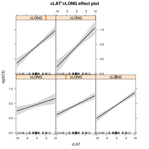
library(effects)
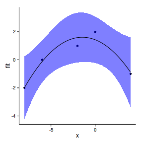
plot(allEffects(paruelo.lm))

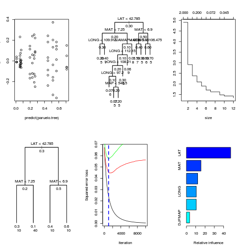
library(tree)
paruelo.tree <- tree(C3~LAT+LONG+MAP+MAT+
  JJAMAP+DJFMAP, data=paruelo, mindev=0)
plot(residuals(paruelo.tree)~predict(paruelo.tree))
plot(paruelo.tree, type="uniform")
text(paruelo.tree,cex=1, all=T)
text(paruelo.tree,lab=paste("n"),cex=1,adj=c(0,2), splits=F)


plot(prune.tree(paruelo.tree))

paruelo.tree.prune<-prune.tree(paruelo.tree, best=4)
plot(paruelo.tree.prune, type="uniform")
text(paruelo.tree.prune,cex=1, all=T)
text(paruelo.tree.prune,lab=paste("n"),cex=1,adj=c(0,2), splits=F)


library(gbm)
paruelo.gbm <- gbm(C3~LAT+LONG+MAP+MAT+JJAMAP+DJFMAP,
       data=paruelo,
       interaction.depth=3,
       train=0.5,
       cv.folds=3,
       n.minobsinnode=2,
       n.trees=10000)

Distribution not specified, assuming gaussian ...

paruelo.gbm <- gbm(C3~LAT+LONG+MAP+MAT+JJAMAP+DJFMAP,
       data=paruelo,
       interaction.depth=7,
       train=0.5,
       cv.folds=3,
       n.minobsinnode=2,
       n.trees=10000)

Distribution not specified, assuming gaussian ...

#paruelo.gbm <- gbm(C3~LAT + LONG + MAP + MAT + JJAMAP + DJFMAP, data=paruelo,
#                   interaction.depth=3, cv.folds=3, dist="bernoulli")

best.iter <- gbm.perf(paruelo.gbm,
  method="cv") 
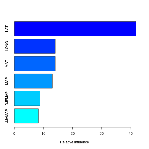
print(best.iter)

[1] 1035

summary(paruelo.gbm,n.trees=best.iter) #see graph

          var rel.inf
LAT       LAT  47.607
MAT       MAT  15.630
MAP       MAP  12.095
LONG     LONG  10.642
JJAMAP JJAMAP  10.597
DJFMAP DJFMAP   3.429

par(mfrow=c(2,3))
plot(paruelo.gbm, 1, best.iter)
plot(paruelo.gbm, 2, best.iter)
plot(paruelo.gbm, 3, best.iter)
plot(paruelo.gbm, 4, best.iter)
plot(paruelo.gbm, 5, best.iter)
plot(paruelo.gbm, 6, best.iter)

plot(paruelo.gbm, c(2,1), best.iter)

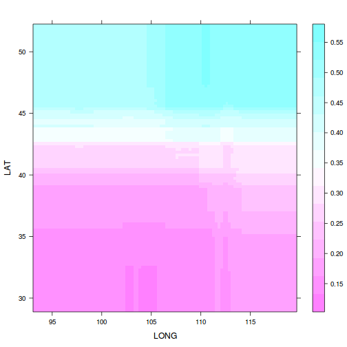
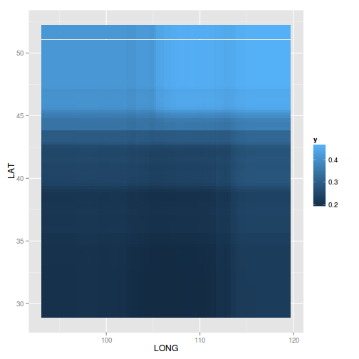
pp<-plot(paruelo.gbm, c(2,1), best.iter,
         return.grid=TRUE)

library(ggplot2)
ggplot(pp, aes(y=LAT, x=LONG, fill=y))+
  geom_tile()

#scatter3d(x=pp$LONG, y=pp$LAT, z=pp$y)
library(scatterplot3d)
scatterplot3d(x=pp$LONG, y=pp$LAT, z=pp$y, angle=24)
with(pp[1:20,],persp(x=LONG, y=LAT, z=y))

Error: increasing 'x' and 'y' values expected

xyz <- with(pp,unique(cbind(x=LONG,y=LAT,z=y)))
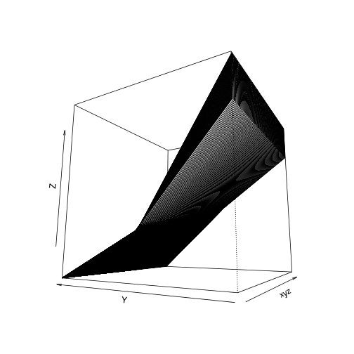
persp(xyz, theta=-60, phi=-10)



##      tree.screens()
##      plot(paruelo.tree)
##      text(paruelo.tree)
##      tile.tree(paruelo.tree, paruelo$LAT)
##      #tile.tree(paruelo.tree, paruelo$LONG)
##      close.screen(all = TRUE)

## paruelo.tree1<-prune.tree(paruelo.tree)
## summary(paruelo.tree1)
## paruelo.tree1$frame

## paruelo.tree1<-prune.tree(paruelo.tree,best=2)
## summary(paruelo.tree1)
## paruelo.tree1$frame


## C3.deciles = quantile(paruelo$C3,1:10/10)
## C3.cut = cut(paruelo$C3,breaks=C3.deciles,include.lowest=TRUE)
## plot(paruelo$LONG,paruelo$LAT,col=grey(10:2/11)[C3.cut],pch=20,xlab="Longitude",ylab="Latitude")



## plot(paruelo$LONG,paruelo$LAT,col=grey(10:2/11)[C3.cut],pch=20,xlab="Longitude",ylab="Latitude")
## paruelo.tree1<-prune.tree(paruelo.tree,best=2)
## plot(paruelo$LAT,paruelo$C3,col=grey(10:2/11)[C3.cut],pch=20,xlab="Longitude",ylab="Latitude")

## partition.tree(paruelo.tree1,ordvars=c("LAT"),add=TRUE)
## partition.tree(paruelo.tree1,ordvars=c("LONG","LAT"),add=FALSE)
## plot(paruelo.tree1)
## text(paruelo.tree1, cex=0.75)


## plot(paruelo$C3~paruelo$LAT,col=grey(10:2/11)[C3.cut],pch=20)
## partition.tree(paruelo.tree,ordvars=c("LONG","LAT"),add=TRUE)

Workshop 11: Classification and Regression Trees

Murray Logan

26-011-2013

Limitations of Linear Models

Limitations of Linear Models

Limitations of Linear Models

Classication & Regression Trees

Advantanges

Classication & Regression Trees

Diss-advantanges

Classication & Regression Trees

Classification

Regression

Simple regression trees

Simple regression trees

Simple regression trees

Simple regression trees

Simple regression trees

Simple regression trees

Simple regression trees

Simple regression trees

Simple regression trees

Simple regression trees

Simple regression trees

Pruning

Simple regression trees

Predictions

Classification and Regression Trees

R packages

Classification and Regression Trees

Limitations

Boosted regression Trees

Boosting

Boosted regression Trees

Over fitting

Boosted regression Trees

minimizing square error loss

Boosted regression Trees

Over fitting

Boosted regression Trees

Predictions

Boosted regression Trees

Variable importance

Boosted regression Trees

\(R^2\)

Worked Examples