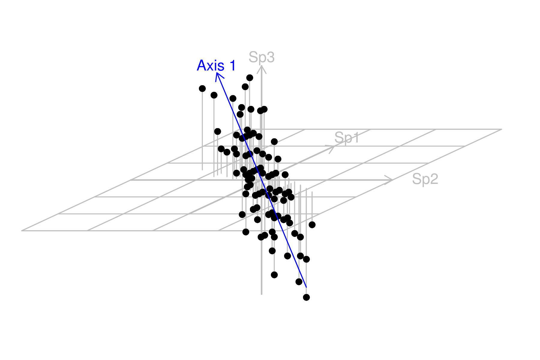
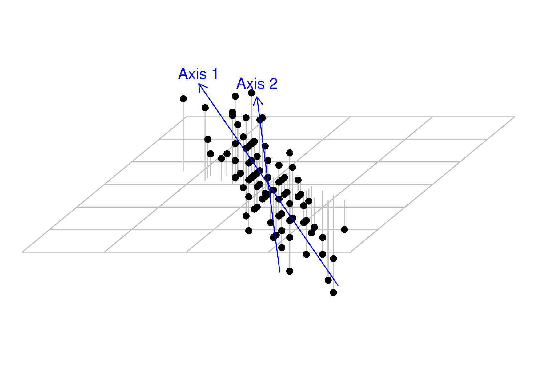
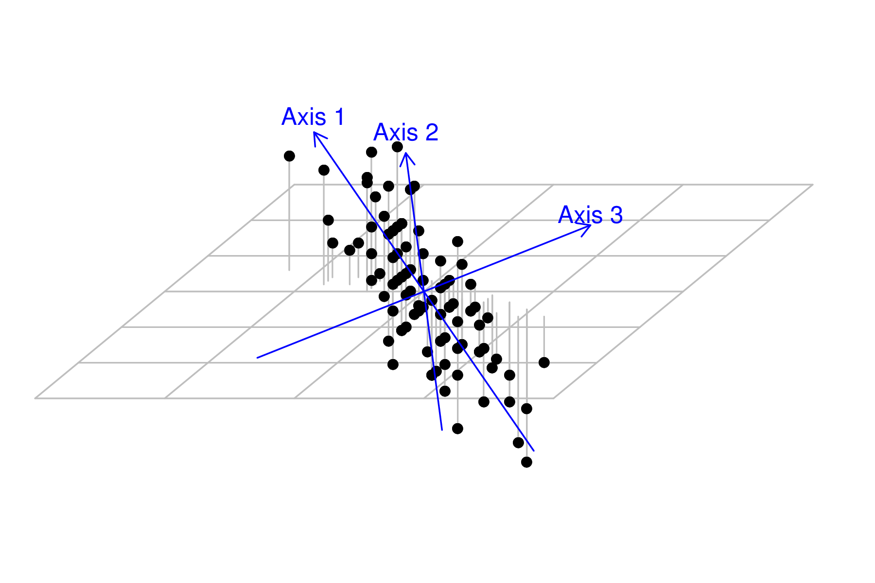
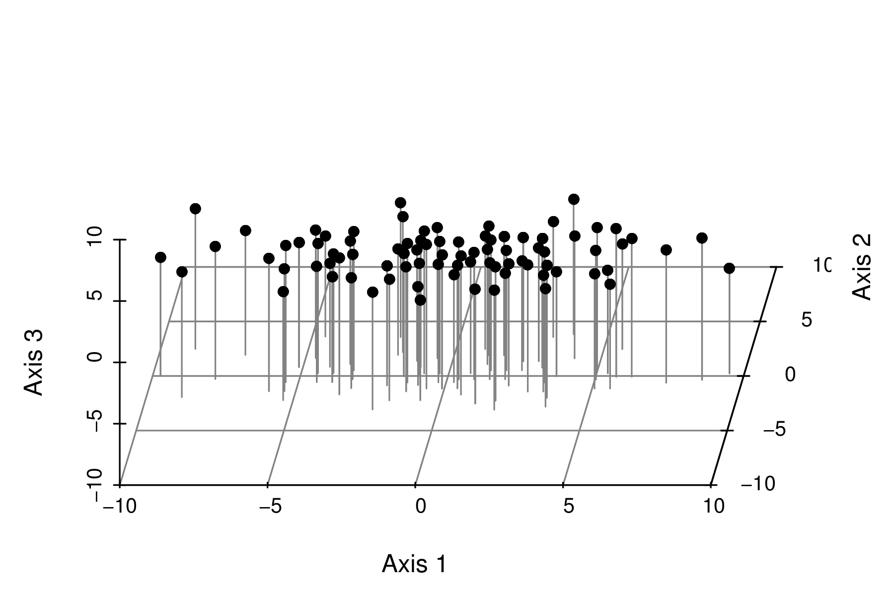
Axis rotation - eigenanalysis
|

|
> # might want to put this in to make the vector arrows and text look nicer..
> geom_text(data=vectors, aes(y=RDA2,x=RDA1,label=Species,
+               hjust=0.5*(1-sign(RDA2)),vjust=0.5*(1-sign(RDA1))), color="red", size=4)
Error in eval(expr, envir, enclos): could not find function "geom_text"| Sp1 | Sp2 | Sp3 | Sp4 | |
|---|---|---|---|---|
| Site1 | 2 | 0 | 0 | 5 |
| Site2 | 13 | 7 | 10 | 5 |
| Site3 | 9 | 5 | 55 | 93 |
| Site4 | 10 | 6 | 76 | 81 |
| Site5 | 0 | 2 | 6 | 0 |
| Sp1 | Sp2 | Sp3 | Sp4 | |
|---|---|---|---|---|
| Site1 | 2 | 0 | 0 | 5 |
| Site2 | 13 | 7 | 10 | 5 |
| Site3 | 9 | 5 | 55 | 93 |
| Site4 | 10 | 6 | 76 | 81 |
| Site5 | 0 | 2 | 6 | 0 |
variance covariance matrix
> var(Y) Sp1 Sp2 Sp3 Sp4
Sp1 30.70 15.00 96.35 117.70
Sp2 15.00 8.50 56.25 62.50
Sp3 96.35 56.25 1153.80 1477.85
Sp4 117.70 62.50 1477.85 2122.20| Sp1 | Sp2 | Sp3 | Sp4 | |
|---|---|---|---|---|
| Site1 | 2 | 0 | 0 | 5 |
| Site2 | 13 | 7 | 10 | 5 |
| Site3 | 9 | 5 | 55 | 93 |
| Site4 | 10 | 6 | 76 | 81 |
| Site5 | 0 | 2 | 6 | 0 |
correlation matrix
> cor(Y) Sp1 Sp2 Sp3 Sp4
Sp1 1.0000000 0.9285656 0.5119379 0.4611202
Sp2 0.9285656 1.0000000 0.5679993 0.4653475
Sp3 0.5119379 0.5679993 1.0000000 0.9444347
Sp4 0.4611202 0.4653475 0.9444347 1.0000000
|
|
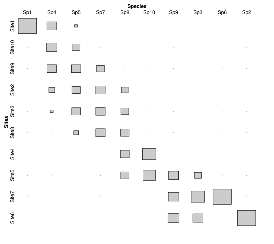
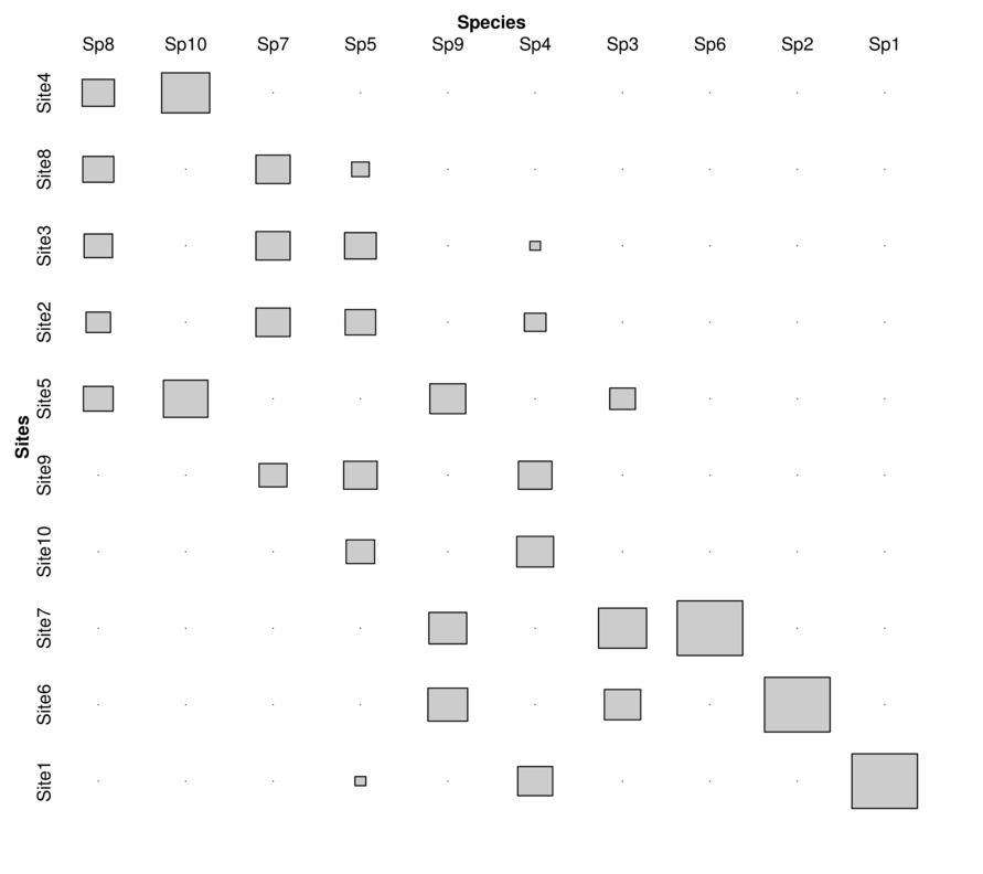
| Sites | Sp1 | Sp2 | Sp3 | Sp4 | Sp5 | Sp6 | Sp7 | Sp8 | Sp9 | Sp10 |
|---|---|---|---|---|---|---|---|---|---|---|
| Site1 | 5 | 0 | 0 | 65 | 5 | 0 | 0 | 0 | 0 | 0 |
| Site2 | 0 | 0 | 0 | 25 | 39 | 0 | 6 | 23 | 0 | 0 |
| Site3 | 0 | 0 | 0 | 6 | 42 | 0 | 6 | 31 | 0 | 0 |
| Site4 | 0 | 0 | 0 | 0 | 0 | 0 | 0 | 40 | 0 | 14 |
| Site5 | 0 | 0 | 6 | 0 | 0 | 0 | 0 | 34 | 18 | 12 |
| Site6 | 0 | 29 | 12 | 0 | 0 | 0 | 0 | 0 | 22 | 0 |
| Site7 | 0 | 0 | 21 | 0 | 0 | 5 | 0 | 0 | 20 | 0 |
| Site8 | 0 | 0 | 0 | 0 | 13 | 0 | 6 | 37 | 0 | 0 |
| Site9 | 0 | 0 | 0 | 60 | 47 | 0 | 4 | 0 | 0 | 0 |
| Site10 | 0 | 0 | 0 | 72 | 34 | 0 | 0 | 0 | 0 | 0 |
> library(vegan)
> data.rda <- rda(data[,-1], scale=TRUE)
> summary(data.rda, scaling=2)
Call:
rda(X = data[, -1], scale = TRUE)

Partitioning of correlations:
              Inertia Proportion
Total              10          1
Unconstrained      10          1

Eigenvalues, and their contribution to the correlations

Importance of components:
                         PC1    PC2    PC3    PC4     PC5
Eigenvalue            3.8220 2.4205 1.6753 1.1701 0.66872
Proportion Explained  0.3822 0.2420 0.1675 0.1170 0.06687
Cumulative Proportion 0.3822 0.6242 0.7918 0.9088 0.97567
                          PC6     PC7    PC8      PC9
Eigenvalue            0.14643 0.06784 0.0280 0.001045
Proportion Explained  0.01464 0.00678 0.0028 0.000100
Cumulative Proportion 0.99031 0.99710 0.9999 1.000000

Scaling 2 for species and site scores
* Species are scaled proportional to eigenvalues
* Sites are unscaled: weighted dispersion equal on all dimensions
* General scaling constant of scores:  3.08007


Species scores

         PC1       PC2      PC3      PC4      PC5       PC6
Sp1  -0.1300 -0.494334 -0.63551  0.08911 -0.50512  0.112154
Sp2   0.5000 -0.157276  0.11701 -0.79900 -0.06343 -0.104375
Sp3   0.9007 -0.170843  0.27779  0.16895 -0.01456  0.038032
Sp4  -0.5235 -0.714165 -0.27820  0.04967  0.27670  0.027303
Sp5  -0.7564 -0.196662  0.47970 -0.01385  0.26323  0.128107
Sp6   0.6212 -0.213901  0.31704  0.63259 -0.04035 -0.101082
Sp7  -0.6311  0.231834  0.61283 -0.01782 -0.32040  0.085889
Sp8  -0.2207  0.925419 -0.04869  0.06432 -0.17279  0.006936
Sp9   0.9110 -0.009745  0.12221 -0.14486  0.05298  0.274048
Sp10  0.1964  0.702341 -0.54197  0.08330  0.30368  0.063979


Site scores (weighted sums of species scores)

            PC1     PC2     PC3       PC4     PC5     PC6
Site1  -0.38988 -1.4830 -1.9065  0.267341 -1.5154  0.3365
Site2  -0.88111  0.1838  0.8579 -0.024947 -0.2562  0.4380
Site3  -0.85013  0.5434  0.9979 -0.028670 -0.5856  0.4768
Site4   0.08351  1.5556 -1.2827  0.242057  0.5852 -1.5801
Site5   0.75662  1.2398 -0.8607  0.079914  0.6381  2.1217
Site6   1.50003 -0.4718  0.3510 -2.396989 -0.1903 -0.3131
Site7   1.86374 -0.6417  0.9511  1.897781 -0.1210 -0.3032
Site8  -0.53994  0.8632  0.5845  0.000059 -1.3634 -0.8814
Site9  -0.93105 -0.7920  0.5521 -0.042154  1.1052  0.5402
Site10 -0.61180 -0.9973 -0.2446 0.005608 1.7033 -0.8354> scores(data.rda, choices=1:4,display="species",
+ scaling=0) PC1 PC2 PC3 PC4
Sp1 -0.06824908 -0.326218616 -0.50409421 0.08457936
Sp2 0.26258604 -0.103789073 0.09281608 -0.75834235
Sp3 0.47302827 -0.112742127 0.22034809 0.16035284
Sp4 -0.27494466 -0.471288231 -0.22067476 0.04713954
Sp5 -0.39723499 -0.129780438 0.38050677 -0.01314949
Sp6 0.32625468 -0.141156180 0.25148155 0.60040642
Sp7 -0.33140801 0.152990372 0.48610356 -0.01691299
Sp8 -0.11589293 0.610697873 -0.03862036 0.06104665
Sp9 0.47844118 -0.006430814 0.09693508 -0.13748918
Sp10 0.10312211 0.463485199 -0.42989602 0.07906481
attr(,"const")
[1] 3.08007> scores(data.rda, choices=1:4,display="sites",
+ scaling=0) PC1 PC2 PC3 PC4
Site1 -0.12658001 -0.48148365 -0.61898528 8.679697e-02
Site2 -0.28606925 0.05966779 0.27853408 -8.099421e-03
Site3 -0.27600945 0.17642036 0.32398109 -9.308103e-03
Site4 0.02711372 0.50505835 -0.41646556 7.858829e-02
Site5 0.24564899 0.40253243 -0.27942593 2.594538e-02
Site6 0.48701231 -0.15318789 0.11397034 -7.782255e-01
Site7 0.60509708 -0.20834002 0.30879819 6.161486e-01
Site8 -0.17530145 0.28025505 0.18975585 1.915695e-05
Site9 -0.30228092 -0.25712656 0.17925008 -1.368605e-02
Site10 -0.19863101 -0.32379586 -0.07941286 1.820656e-03
attr(,"const")
[1] 3.08007> summary(data.rda, scaling=2)$species PC1 PC2 PC3 PC4
Sp1 -0.1299584 -0.494334499 -0.63550605 0.08911359
Sp2 0.5000107 -0.157276491 0.11701221 -0.79899645
Sp3 0.9007303 -0.170843477 0.27779043 0.16894923
Sp4 -0.5235437 -0.714165347 -0.27820226 0.04966665
Sp5 -0.7564064 -0.196662436 0.47970072 -0.01385442
Sp6 0.6212472 -0.213900635 0.31704004 0.63259371
Sp7 -0.6310600 0.231833546 0.61282545 -0.01781968
Sp8 -0.2206808 0.925419372 -0.04868826 0.06431931
Sp9 0.9110374 -0.009744917 0.12220500 -0.14485986
Sp10 0.1963629 0.702341045 -0.54196521 0.08330341
PC5 PC6
Sp1 -0.50512223 0.112154283
Sp2 -0.06343012 -0.104375378
Sp3 -0.01455567 0.038032290
Sp4 0.27669707 0.027303319
Sp5 0.26323433 0.128106871
Sp6 -0.04034569 -0.101081509
Sp7 -0.32040479 0.085888650
Sp8 -0.17279101 0.006935947
Sp9 0.05297717 0.274047718
Sp10 0.30367672 0.063978952> summary(data.rda, scaling=1)$species PC1 PC2 PC3 PC4
Sp1 -0.2102120 -1.00477627 -1.5526456 0.26051036
Sp2 0.8087835 -0.31967764 0.2858800 -2.33574773
Sp3 1.4569603 -0.34725367 0.6786876 0.49389803
Sp4 -0.8468489 -1.45160088 -0.6796938 0.14519308
Sp5 -1.2235117 -0.39973287 1.1719876 -0.04050134
Sp6 1.0048873 -0.43477095 0.7745809 1.84929399
Sp7 -1.0207599 0.47122110 1.4972331 -0.05209320
Sp8 -0.3569584 1.88099237 -0.1189534 0.18802797
Sp9 1.4736325 -0.01980736 0.2985669 -0.42347634
Sp10 0.3176233 1.42756699 -1.3241099 0.24352519
PC5 PC6
Sp1 -1.95331854 0.92683727
Sp2 -0.24528563 -0.86255279
Sp3 -0.05628709 0.31429690
Sp4 1.06999353 0.22563323
Sp5 1.01793280 1.05866864
Sp6 -0.15601764 -0.83533243
Sp7 -1.23901222 0.70977941
Sp8 -0.66818654 0.05731831
Sp9 0.20486387 2.26471634
Sp10 1.17432441 0.52871879> summary(data.rda, scaling=2)$sites PC1 PC2 PC3 PC4
Site1 -0.38987532 -1.4830035 -1.9065182 2.673408e-01
Site2 -0.88111339 0.1837810 0.8579046 -2.494679e-02
Site3 -0.85012850 0.5433871 0.9978845 -2.866961e-02
Site4 0.08351215 1.5556152 -1.2827432 2.420575e-01
Site5 0.75661614 1.2398282 -0.8606515 7.991361e-02
Site6 1.50003214 -0.4718295 0.3510366 -2.396989e+00
Site7 1.86374152 -0.6417019 0.9511201 1.897781e+00
Site8 -0.53994078 0.8632053 0.5844614 5.900474e-05
Site9 -0.93104649 -0.7919679 0.5521028 -4.215398e-02
Site10 -0.61179747 -0.9973140 -0.2445972 5.607748e-03
PC5 PC6
Site1 -1.5153667 0.3364629
Site2 -0.2561519 0.4380054
Site3 -0.5855919 0.4768201
Site4 0.5851709 -1.5800521
Site5 0.6380907 2.1216597
Site6 -0.1902904 -0.3131261
Site7 -0.1210371 -0.3032445
Site8 -1.3633582 -0.8813587
Site9 1.1052341 0.5401866
Site10 1.7033003 -0.8353532> summary(data.rda, scaling=1)$sites PC1 PC2 PC3 PC4
Site1 -0.24103094 -0.72961495 -0.7803480 9.145008e-02
Site2 -0.54472693 0.09041742 0.3511449 -8.533624e-03
Site3 -0.52557128 0.26733811 0.4084394 -9.807103e-03
Site4 0.05162936 0.76533880 -0.5250336 8.280135e-02
Site5 0.46775954 0.60997643 -0.3522692 2.733629e-02
Site6 0.92735841 -0.23213286 0.1436812 -8.199456e-01
Site7 1.15221289 -0.31570749 0.3892985 6.491799e-01
Site8 -0.33380527 0.42468374 0.2392231 2.018393e-05
Site9 -0.57559686 -0.38963603 0.2259786 -1.441974e-02
Site10 -0.37822892 -0.49066318 -0.1001149 1.918260e-03
PC5 PC6
Site1 -0.39186922 0.04071454
Site2 -0.06624011 0.05300195
Site3 -0.15143228 0.05769882
Site4 0.15132341 -0.19119820
Site5 0.16500833 0.25673679
Site6 -0.04920851 -0.03789062
Site7 -0.03129982 -0.03669487
Site8 -0.35256027 -0.10665104
Site9 0.28581018 0.06536664
Site10 0.44046828 -0.10108402 PC1 PC2 PC3 PC4 PC5
3.822030054 2.420488947 1.675308207 1.170140005 0.668723871
PC6 PC7 PC8 PC9
0.146428210 0.067836468 0.027999675 0.001044563 PC1 PC2 PC3 PC4 PC5
3.822030054 2.420488947 1.675308207 1.170140005 0.668723871
PC6 PC7 PC8 PC9
0.146428210 0.067836468 0.027999675 0.001044563 PC1 PC2 PC3 PC4 PC5 PC6 PC7 PC8
38.22 62.43 79.18 90.88 97.57 99.03 99.71 99.99
PC9
100.00 PC1 PC2 PC3 PC4 PC5
3.822030054 2.420488947 1.675308207 1.170140005 0.668723871
PC6 PC7 PC8 PC9
0.146428210 0.067836468 0.027999675 0.001044563 PC1 PC2 PC3 PC4 PC5 PC6 PC7 PC8
38.22 62.43 79.18 90.88 97.57 99.03 99.71 99.99
PC9
100.00 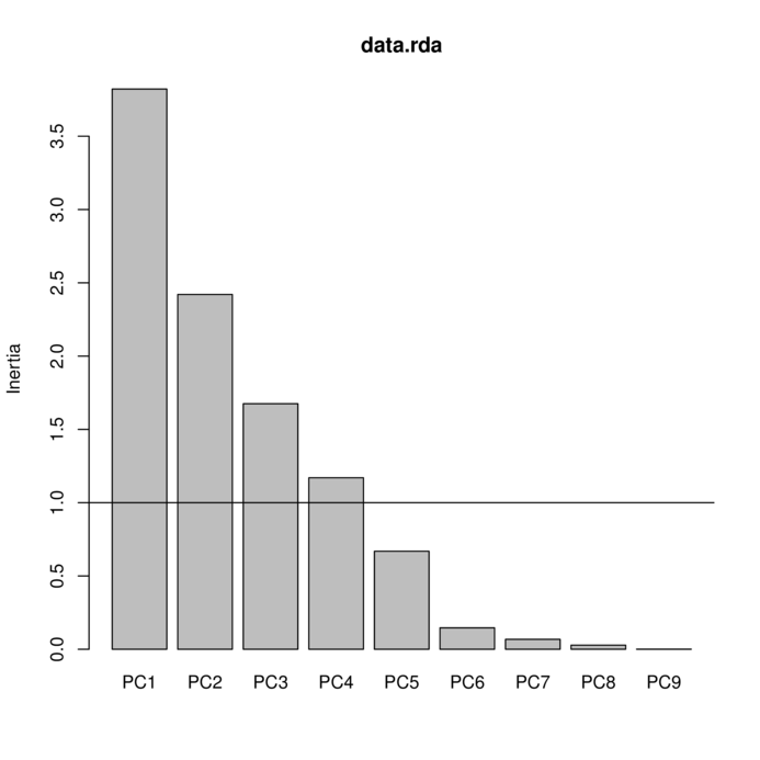
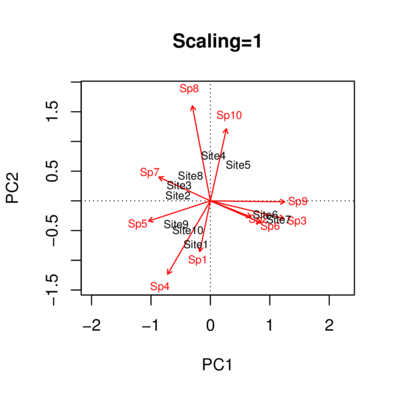
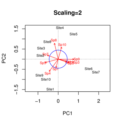
> plot(data.rda)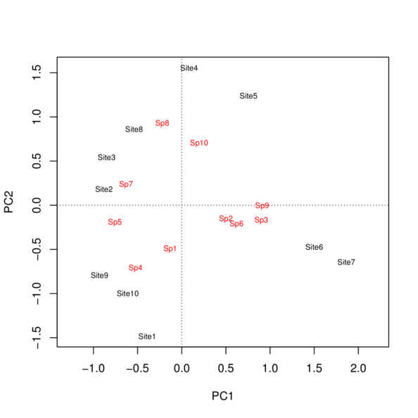
|
|
| Site | pH | Slope | Pressure | Altitude | Substrate |
|---|---|---|---|---|---|
| Site1 | 6 | 4 | 101325 | 2 | Quartz |
| Site2 | 7 | 9 | 101352 | 510 | Shale |
| Site3 | 7 | 9 | 101356 | 546 | Shale |
| Site4 | 7 | 7 | 101372 | 758 | Shale |
| Site5 | 7 | 6 | 101384 | 813 | Shale |
| Site6 | 8 | 8 | 101395 | 856 | Quartz |
| Site7 | 8 | 0 | 101396 | 854 | Quartz |
| Site8 | 7 | 12 | 101370 | 734 | Shale |
| Site9 | 8 | 8 | 101347 | 360 | Quartz |
| Site10 | 6 | 2 | 101345 | 356 | Quartz |


> library(car)
> vif(lm(data.rda$CA$u[,1]~Slope+Altitude+Pressure+
+   Substrate+pH, data=enviro))
Slope Altitude Pressure Substrate pH
2.187796 52.754368 45.804821 5.118418 1.976424 > library(car)
> vif(lm(data.rda$CA$u[,1]~Slope+Altitude+Pressure+
+ Substrate+pH, data=enviro)) Slope Altitude Pressure Substrate pH
2.187796 52.754368 45.804821 5.118418 1.976424 > vif(lm(data.rda$CA$u[,1]~Slope+Altitude+Substrate+
+ pH, data=enviro)) Slope Altitude Substrate pH
2.116732 1.830014 2.636302 1.968157 Three responses
> data.lm<-lm(data.rda$CA$u[,1:3]~Slope+Altitude+Substrate+
+ pH, data=enviro)> summary(data.lm)[[1]]$coef Estimate Std. Error t value
(Intercept) 0.180787455 0.8121647657 0.2225995
Slope -0.021324431 0.0259195942 -0.8227147
Altitude 0.001127743 0.0003074246 3.6683553
SubstrateShale -0.326063277 0.1951991407 -1.6704135
pH -0.075386061 0.1322828004 -0.5698856
Pr(>|t|)
(Intercept) 0.83265462
Slope 0.44811475
Altitude 0.01446816
SubstrateShale 0.15570393
pH 0.59340544> summary(data.lm)[[1]]$coef Estimate Std. Error t value
(Intercept) 0.180787455 0.8121647657 0.2225995
Slope -0.021324431 0.0259195942 -0.8227147
Altitude 0.001127743 0.0003074246 3.6683553
SubstrateShale -0.326063277 0.1951991407 -1.6704135
pH -0.075386061 0.1322828004 -0.5698856
Pr(>|t|)
(Intercept) 0.83265462
Slope 0.44811475
Altitude 0.01446816
SubstrateShale 0.15570393
pH 0.59340544> summary(data.lm)[[2]]$coef Estimate Std. Error t value
(Intercept) -0.8361050965 0.513155076 -1.6293420
Slope -0.0074535542 0.016376937 -0.4551250
Altitude 0.0003381004 0.000194242 1.7406140
SubstrateShale 0.5480944974 0.123333878 4.4439898
pH 0.0589810882 0.083581058 0.7056753
Pr(>|t|)
(Intercept) 0.164169419
Slope 0.668099646
Altitude 0.142232378
SubstrateShale 0.006739835
pH 0.511901060> summary(data.lm)[[1]]$coef Estimate Std. Error t value
(Intercept) 0.180787455 0.8121647657 0.2225995
Slope -0.021324431 0.0259195942 -0.8227147
Altitude 0.001127743 0.0003074246 3.6683553
SubstrateShale -0.326063277 0.1951991407 -1.6704135
pH -0.075386061 0.1322828004 -0.5698856
Pr(>|t|)
(Intercept) 0.83265462
Slope 0.44811475
Altitude 0.01446816
SubstrateShale 0.15570393
pH 0.59340544> summary(data.lm)[[2]]$coef Estimate Std. Error t value
(Intercept) -0.8361050965 0.513155076 -1.6293420
Slope -0.0074535542 0.016376937 -0.4551250
Altitude 0.0003381004 0.000194242 1.7406140
SubstrateShale 0.5480944974 0.123333878 4.4439898
pH 0.0589810882 0.083581058 0.7056753
Pr(>|t|)
(Intercept) 0.164169419
Slope 0.668099646
Altitude 0.142232378
SubstrateShale 0.006739835
pH 0.511901060> summary(data.lm)[[3]]$coef Estimate Std. Error t value
(Intercept) -1.1148132894 1.6441465097 -0.6780498
Slope 0.0225742272 0.0524716316 0.4302177
Altitude 0.0003341175 0.0006223505 0.5368638
SubstrateShale -0.0908322738 0.3951611784 -0.2298613
pH 0.1162957219 0.2677933269 0.4342742
Pr(>|t|)
(Intercept) 0.5278434
Slope 0.6849494
Altitude 0.6143806
SubstrateShale 0.8273072
pH 0.6821907 

| Sites | Sp1 | Sp2 | Sp3 | Sp4 | Sp5 | Sp6 | Sp7 | Sp8 | Sp9 | Sp10 |
|---|---|---|---|---|---|---|---|---|---|---|
| Site1 | 5 | 0 | 0 | 65 | 5 | 0 | 0 | 0 | 0 | 0 |
| Site2 | 0 | 0 | 0 | 25 | 39 | 0 | 6 | 23 | 0 | 0 |
| Site3 | 0 | 0 | 0 | 6 | 42 | 0 | 6 | 31 | 0 | 0 |
| Site4 | 0 | 0 | 0 | 0 | 0 | 0 | 0 | 40 | 0 | 14 |
| Site5 | 0 | 0 | 6 | 0 | 0 | 0 | 0 | 34 | 18 | 12 |
| Site6 | 0 | 29 | 12 | 0 | 0 | 0 | 0 | 0 | 22 | 0 |
| Site7 | 0 | 0 | 21 | 0 | 0 | 5 | 0 | 0 | 20 | 0 |
| Site8 | 0 | 0 | 0 | 0 | 13 | 0 | 6 | 37 | 0 | 0 |
| Site9 | 0 | 0 | 0 | 60 | 47 | 0 | 4 | 0 | 0 | 0 |
| Site10 | 0 | 0 | 0 | 72 | 34 | 0 | 0 | 0 | 0 | 0 |
| Site | pH | Slope | Pressure | Altitude | Substrate |
|---|---|---|---|---|---|
| Site1 | 6 | 4 | 101325 | 2 | Quartz |
| Site2 | 7 | 9 | 101352 | 510 | Shale |
| Site3 | 7 | 9 | 101356 | 546 | Shale |
| Site4 | 7 | 7 | 101372 | 758 | Shale |
| Site5 | 7 | 6 | 101384 | 813 | Shale |
| Site6 | 8 | 8 | 101395 | 856 | Quartz |
| Site7 | 8 | 0 | 101396 | 854 | Quartz |
| Site8 | 7 | 12 | 101370 | 734 | Shale |
| Site9 | 8 | 8 | 101347 | 360 | Quartz |
| Site10 | 6 | 2 | 101345 | 356 | Quartz |
Call:
rda(formula = data.sp ~ Slope + Altitude + Substrate + pH, data = enviro,      scale = TRUE)

Partitioning of correlations:
              Inertia Proportion
Total          10.000     1.0000
Constrained     6.803     0.6803
Unconstrained   3.197     0.3197

Eigenvalues, and their contribution to the correlations

Importance of components:
                        RDA1   RDA2    RDA3    RDA4    PC1
Eigenvalue            3.2736 2.3246 0.94753 0.25721 1.6686
Proportion Explained  0.3274 0.2325 0.09475 0.02572 0.1669
Cumulative Proportion 0.3274 0.5598 0.65457 0.68029 0.8471
                          PC2     PC3     PC4     PC5
Eigenvalue            0.98370 0.42545 0.08546 0.03393
Proportion Explained  0.09837 0.04255 0.00855 0.00339
Cumulative Proportion 0.94552 0.98806 0.99661 1.00000

Accumulated constrained eigenvalues
Importance of components:
                        RDA1   RDA2   RDA3    RDA4
Eigenvalue            3.2736 2.3246 0.9475 0.25721
Proportion Explained  0.4812 0.3417 0.1393 0.03781
Cumulative Proportion 0.4812 0.8229 0.9622 1.00000

Scaling 2 for species and site scores
* Species are scaled proportional to eigenvalues
* Sites are unscaled: weighted dispersion equal on all dimensions
* General scaling constant of scores:  3.08007


Species scores

        RDA1     RDA2     RDA3      RDA4      PC1      PC2
Sp1  -0.4625  0.53068 -0.06866  0.253791 -0.45077 -0.42289
Sp2   0.4496  0.17767  0.70674  0.047286 -0.20609  0.09076
Sp3   0.8605  0.14459 -0.07160 -0.073481  0.01511 -0.39443
Sp4  -0.5038  0.73807 -0.17492 -0.053209  0.09486  0.28160
Sp5  -0.5412  0.06265 -0.02421 -0.300536  0.66564  0.28803
Sp6   0.6378  0.16243 -0.37542 -0.090719  0.25610 -0.50570
Sp7  -0.5134 -0.42926  0.28574 -0.206257  0.58746 -0.17367
Sp8  -0.1998 -0.91143 -0.04662  0.156707 -0.11938  0.04756
Sp9   0.8211  0.01396  0.04385 -0.058407 -0.23106 -0.21288
Sp10  0.1332 -0.53007 -0.36293  0.008524 -0.63767  0.30795


Site scores (weighted sums of species scores)

                RDA1    RDA2     RDA3    RDA4     PC1
Site Site1  -0.79327  1.6804 -0.57398  3.8613 -1.3523
Site Site2  -0.83161 -0.4019  0.46703 -2.1620  1.0017
Site Site3  -0.78597 -0.7893  0.56036 -1.9250  1.0466
Site Site4   0.03055 -1.3306 -1.05657  2.8638 -1.2801
Site Site5   0.75712 -1.0386 -0.86818  1.9420 -1.2800
Site Site6   1.58269  0.5814  2.55098  0.9117 -0.6183
Site Site7   2.06536  0.6400 -1.36534 -1.2030  0.7683
Site Site8  -0.52322 -1.0342  0.62009  0.1174  0.5119
Site Site9  -0.88977  0.6559  0.08146 -3.1438  0.1980
Site Site10 -0.61188  1.0369 -0.41586 -1.2624  1.0043
                PC2
Site Site1  -1.2687
Site Site2  -0.3103
Site Site3  -0.2950
Site Site4   0.9220
Site Site5   0.2638
Site Site6   0.2723
Site Site7  -1.5171
Site Site8  -0.5805
Site Site9   0.5848
Site Site10  1.9287


Site constraints (linear combinations of constraining variables)

               RDA1    RDA2     RDA3    RDA4     PC1
Site Site1  -1.3876  1.5920 -0.20599  0.7614 -1.3523
Site Site2  -0.8984 -0.7156  0.06891  0.3099  1.0017
Site Site3  -0.7330 -0.7750 -0.18965  0.1650  1.0466
Site Site4   0.1311 -1.0148 -0.39673  0.1773 -1.2801
Site Site5   0.4262 -1.1215 -1.11563 -0.1698 -1.2800
Site Site6   1.3488  0.5330  2.12023  0.1419 -0.6183
Site Site7   1.9135  0.4873 -1.12627 -0.2722  0.7683
Site Site8  -0.2790 -0.9677  1.35583  0.3537  0.5119
Site Site9  -0.6631  0.7367  0.11148 -2.6608  0.1980
Site Site10  0.1414  1.2455 -0.62218  1.1935  1.0043
                PC2
Site Site1  -1.2687
Site Site2  -0.3103
Site Site3  -0.2950
Site Site4   0.9220
Site Site5   0.2638
Site Site6   0.2723
Site Site7  -1.5171
Site Site8  -0.5805
Site Site9   0.5848
Site Site10  1.9287


Biplot scores for constraining variables

                  RDA1    RDA2     RDA3     RDA4 PC1 PC2
Slope          -0.4012 -0.5892  0.66815 -0.21310   0   0
Altitude        0.7686 -0.6192  0.15152 -0.05368   0   0
SubstrateShale -0.2779 -0.9434 -0.05693  0.17170   0   0
pH              0.3768 -0.1196  0.18204 -0.90031   0   0


Centroids for factor constraints

                   RDA1    RDA2     RDA3    RDA4 PC1 PC2
SubstrateQuartz  0.2706  0.9189  0.05545 -0.1672   0   0
SubstrateShale -0.2706 -0.9189 -0.05545 0.1672 0 0> summary(data.rda, scaling=2)$biplot RDA1 RDA2 RDA3
Slope -0.4012090 -0.5892359 0.66814874
Altitude 0.7686367 -0.6191599 0.15151633
SubstrateShale -0.2778501 -0.9434386 -0.05693409
pH 0.3768405 -0.1195525 0.18203818
RDA4 PC1 PC2
Slope -0.21309525 0 0
Altitude -0.05367921 0 0
SubstrateShale 0.17170182 0 0
pH -0.90031137 0 0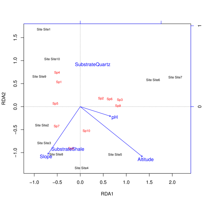
Permutation ANOVA
Permutation test for rda under reduced model
Permutation: free
Number of permutations: 999

Model: rda(formula = data.sp ~ Slope + Altitude + Substrate + pH, data = enviro, scale = TRUE)
         Df Variance      F Pr(>F)
Model     4   6.8029 2.6598  0.007 **
Residual  5   3.1971
---
Signif. codes:
0 '***' 0.001 '**' 0.01 '*' 0.05 '.' 0.1 ' ' 1
Permutation ANOVA (Type III SS)
Permutation test for rda under reduced model
Marginal effects of terms
Permutation: free
Number of permutations: 999

Model: rda(formula = data.sp ~ Slope + Altitude + Substrate + pH, data = enviro, scale = TRUE)
          Df Variance      F Pr(>F)
Slope      1   1.0065 1.5741  0.159
Altitude   1   2.2199 3.4718  0.002 **
Substrate  1   1.5685 2.4531  0.033 *
pH         1   0.4273 0.6683  0.694
Residual   5   3.1971
---
Signif. codes:
0 '***' 0.001 '**' 0.01 '*' 0.05 '.' 0.1 ' ' 1Stepwise model selection
          Df    AIC      F Pr(>F)
<none>       20.569
Slope      1 21.306 1.5741  0.170
Altitude   1 23.842 3.4718  0.005 **
Substrate  1 22.561 2.4531  0.025 *
pH         1 19.823 0.6683  0.645
---
Signif. codes:
0 '***' 0.001 '**' 0.01 '*' 0.05 '.' 0.1 ' ' 1PCA

> data <- decostand(data[,-1],method="total",MARGIN=2)
> data
Sp1 Sp2 Sp3 Sp4 Sp5 Sp6
Site1 1 0 0.0000000 0.28508772 0.02777778 0
Site2 0 0 0.0000000 0.10964912 0.21666667 0
Site3 0 0 0.0000000 0.02631579 0.23333333 0
Site4 0 0 0.0000000 0.00000000 0.00000000 0
Site5 0 0 0.1538462 0.00000000 0.00000000 0
Site6 0 1 0.3076923 0.00000000 0.00000000 0
Site7 0 0 0.5384615 0.00000000 0.00000000 1
Site8 0 0 0.0000000 0.00000000 0.07222222 0
Site9 0 0 0.0000000 0.26315789 0.26111111 0
Site10 0 0 0.0000000 0.31578947 0.18888889 0
Sp7 Sp8 Sp9 Sp10
Site1 0.0000000 0.0000000 0.0000000 0.0000000
Site2 0.2727273 0.1393939 0.0000000 0.0000000
Site3 0.2727273 0.1878788 0.0000000 0.0000000
Site4 0.0000000 0.2424242 0.0000000 0.5384615
Site5 0.0000000 0.2060606 0.3000000 0.4615385
Site6 0.0000000 0.0000000 0.3666667 0.0000000
Site7 0.0000000 0.0000000 0.3333333 0.0000000
Site8 0.2727273 0.2242424 0.0000000 0.0000000
Site9 0.1818182 0.0000000 0.0000000 0.0000000
Site10 0.0000000 0.0000000 0.0000000 0.0000000
Minimize \(\chi^2\) residuals
> data.ca <- cca(data)
> summary(data.ca)
Call:
cca(X = data)

Partitioning of mean squared contingency coefficient:
              Inertia Proportion
Total           3.256          1
Unconstrained   3.256          1

Eigenvalues, and their contribution to the mean squared contingency coefficient

Importance of components:
                         CA1    CA2    CA3    CA4     CA5
Eigenvalue            0.9463 0.7823 0.6214 0.5784 0.26286
Proportion Explained  0.2906 0.2402 0.1908 0.1776 0.08073
Cumulative Proportion 0.2906 0.5309 0.7217 0.8994 0.98009
                          CA6     CA7      CA8
Eigenvalue            0.04315 0.01551 0.006164
Proportion Explained  0.01325 0.00476 0.001890
Cumulative Proportion 0.99334 0.99811 1.000000

Scaling 2 for species and site scores
* Species are scaled proportional to eigenvalues
* Sites are unscaled: weighted dispersion equal on all dimensions


Species scores

         CA1     CA2      CA3      CA4      CA5       CA6
Sp1  -1.4446  1.8842 -0.86530  0.03061 -0.47720 -0.006432
Sp2   1.1313  0.5380  0.52836  1.74914 -0.05360  0.247953
Sp3   1.0302  0.3407  0.16160 -0.32148  0.00978 -0.135905
Sp4  -1.1395  0.2409  0.47543 -0.02254  1.06125  0.022650
Sp5  -0.9094 -0.6375  0.85632 -0.03372  0.35896 -0.014035
Sp6   1.1250  0.5162  0.37542 -1.61102 -0.05869  0.265755
Sp7  -0.7780 -0.9688  0.78276 -0.02684 -0.79494 -0.033065
Sp8  -0.2565 -1.0628 -0.43367  0.02821 -0.55703  0.053469
Sp9   0.9388  0.1688 -0.07722  0.11955  0.07364 -0.513328
Sp10  0.3026 -1.0196 -1.80371  0.08808  0.43783  0.112936


Site scores (weighted averages of species scores)

           CA1     CA2     CA3      CA4      CA5       CA6
Site1  -1.4446  1.8842 -0.8653  0.03061 -0.47720 -0.006432
Site2  -0.8156 -0.9072  0.8514 -0.03082 -0.51678 -0.066579
Site3  -0.7373 -1.0761  0.7693 -0.02515 -1.10800 -0.053106
Site4   0.1364 -1.3205 -2.2180  0.12014  0.49068  2.189249
Site5   0.4965 -0.6686 -1.3203  0.05068  0.37618 -2.309429
Site6   1.1313  0.5380  0.5284  1.74914 -0.05360  0.247953
Site7   1.1250  0.5162  0.3754 -1.61102 -0.05869  0.265755
Site8  -0.6227 -1.2320  0.5034 -0.01041 -2.11065  0.079747
Site9  -1.0159 -0.5055  1.1190 -0.04803  1.23098 -0.121948
Site10 -1.1131 -0.1123  0.9944 -0.04620  3.03739  0.206699
> data.ca <- cca(data)
> summary(data.ca)
Call:
cca(X = data)

Partitioning of mean squared contingency coefficient:
              Inertia Proportion
Total           3.256          1
Unconstrained   3.256          1

Eigenvalues, and their contribution to the mean squared contingency coefficient

Importance of components:
                         CA1    CA2    CA3    CA4     CA5
Eigenvalue            0.9463 0.7823 0.6214 0.5784 0.26286
Proportion Explained  0.2906 0.2402 0.1908 0.1776 0.08073
Cumulative Proportion 0.2906 0.5309 0.7217 0.8994 0.98009
                          CA6     CA7      CA8
Eigenvalue            0.04315 0.01551 0.006164
Proportion Explained  0.01325 0.00476 0.001890
Cumulative Proportion 0.99334 0.99811 1.000000

Scaling 2 for species and site scores
* Species are scaled proportional to eigenvalues
* Sites are unscaled: weighted dispersion equal on all dimensions


Species scores

         CA1     CA2      CA3      CA4      CA5       CA6
Sp1  -1.4446  1.8842 -0.86530  0.03061 -0.47720 -0.006432
Sp2   1.1313  0.5380  0.52836  1.74914 -0.05360  0.247953
Sp3   1.0302  0.3407  0.16160 -0.32148  0.00978 -0.135905
Sp4  -1.1395  0.2409  0.47543 -0.02254  1.06125  0.022650
Sp5  -0.9094 -0.6375  0.85632 -0.03372  0.35896 -0.014035
Sp6   1.1250  0.5162  0.37542 -1.61102 -0.05869  0.265755
Sp7  -0.7780 -0.9688  0.78276 -0.02684 -0.79494 -0.033065
Sp8  -0.2565 -1.0628 -0.43367  0.02821 -0.55703  0.053469
Sp9   0.9388  0.1688 -0.07722  0.11955  0.07364 -0.513328
Sp10  0.3026 -1.0196 -1.80371  0.08808  0.43783  0.112936


Site scores (weighted averages of species scores)

           CA1     CA2     CA3      CA4      CA5       CA6
Site1  -1.4446  1.8842 -0.8653  0.03061 -0.47720 -0.006432
Site2  -0.8156 -0.9072  0.8514 -0.03082 -0.51678 -0.066579
Site3  -0.7373 -1.0761  0.7693 -0.02515 -1.10800 -0.053106
Site4   0.1364 -1.3205 -2.2180  0.12014  0.49068  2.189249
Site5   0.4965 -0.6686 -1.3203  0.05068  0.37618 -2.309429
Site6   1.1313  0.5380  0.5284  1.74914 -0.05360  0.247953
Site7   1.1250  0.5162  0.3754 -1.61102 -0.05869  0.265755
Site8  -0.6227 -1.2320  0.5034 -0.01041 -2.11065  0.079747
Site9  -1.0159 -0.5055  1.1190 -0.04803  1.23098 -0.121948
Site10 -1.1131 -0.1123 0.9944 -0.04620 3.03739 0.206699> data.ca$CA$eig CA1 CA2 CA3 CA4 CA5
0.946305134 0.782293787 0.621442179 0.578436060 0.262857400
CA6 CA7 CA8
0.043153975 0.015510825 0.006164366 > mean(data.ca$CA$eig)[1] 0.4070205> data.ca$CA$eig>mean(data.ca$CA$eig) CA1 CA2 CA3 CA4 CA5 CA6 CA7 CA8
TRUE TRUE TRUE TRUE FALSE FALSE FALSE FALSE > data.ca$CA$eig CA1 CA2 CA3 CA4 CA5
0.946305134 0.782293787 0.621442179 0.578436060 0.262857400
CA6 CA7 CA8
0.043153975 0.015510825 0.006164366 > data.ca$CA$eig>0.6 CA1 CA2 CA3 CA4 CA5 CA6 CA7 CA8
TRUE TRUE TRUE FALSE FALSE FALSE FALSE FALSE > screeplot(data.ca)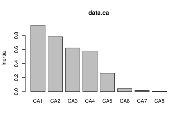
| Site | pH | Slope | Pressure | Altitude | Substrate |
|---|---|---|---|---|---|
| Site1 | 6.1 | 4.2 | 101325 | 2 | Quartz |
| Site2 | 6.7 | 9.2 | 101352 | 510 | Shale |
| Site3 | 6.8 | 8.6 | 101356 | 546 | Shale |
| Site4 | 7.0 | 7.4 | 101372 | 758 | Shale |
| Site5 | 7.2 | 5.8 | 101384 | 813 | Shale |
| Site6 | 7.5 | 8.4 | 101395 | 856 | Quartz |
| Site7 | 7.5 | 0.5 | 101396 | 854 | Quartz |
| Site8 | 7.0 | 11.8 | 101370 | 734 | Shale |
| Site9 | 8.4 | 8.2 | 101347 | 360 | Quartz |
| Site10 | 6.2 | 1.5 | 101345 | 356 | Quartz |
> envfit(data.ca,env=enviro[,-1])
***VECTORS
CA1 CA2 r2 Pr(>r)
pH 0.91731 -0.39818 0.4044 0.244
Slope -0.41261 -0.91091 0.3135 0.355
Pressure 0.98437 -0.17609 0.9833 0.001 ***
Altitude 0.90763 -0.41978 0.9828 0.001 ***
---
Signif. codes:
0 '***' 0.001 '**' 0.01 '*' 0.05 '.' 0.1 ' ' 1
Permutation: free
Number of permutations: 999
***FACTORS:
Centroids:
CA1 CA2
SubstrateQuartz 0.1358 0.6470
SubstrateShale -0.2098 -0.9992
Goodness of fit:
r2 Pr(>r)
Substrate 0.3375 0.033 *
---
Signif. codes:
0 '***' 0.001 '**' 0.01 '*' 0.05 '.' 0.1 ' ' 1
Permutation: free
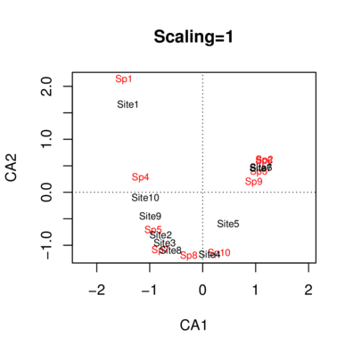
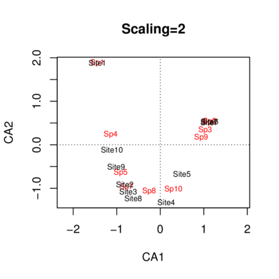
Number of permutations: 999> plot(data.ca)
> plot(envfit(data.ca,env=enviro[,-1]))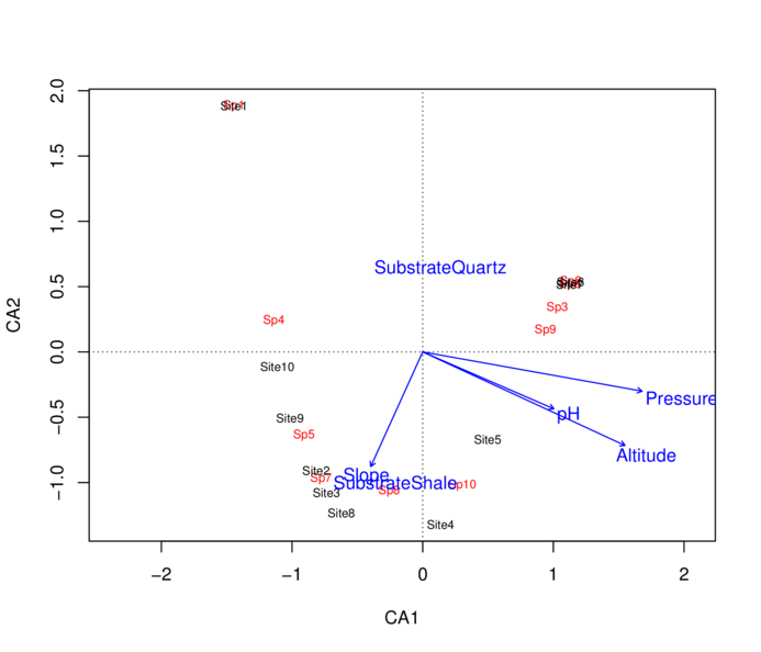
> data.lm <- lm(data.ca$CA$u[,1:3] ~ enviro$Altitude + enviro$Slope+enviro$pH+enviro$Substrate)
> summary(data.lm)
Response CA1 :
Call:
lm(formula = CA1 ~ enviro$Altitude + enviro$Slope + enviro$pH +
enviro$Substrate)
Residuals:
Site1 Site2 Site3 Site4 Site5 Site6
0.422144 0.061252 -0.002323 0.112485 0.232025 0.287221
Site7 Site8 Site9 Site10
-0.002549 -0.403439 -0.161979 -0.544838
Coefficients:
Estimate Std. Error t value
(Intercept) -1.5720999 1.7269003 -0.910
enviro$Altitude 0.0033945 0.0006537 5.193
enviro$Slope -0.0367321 0.0551127 -0.666
enviro$pH -0.0241178 0.2812720 -0.086
enviro$SubstrateShale -0.5363786 0.4150506 -1.292
Pr(>|t|)
(Intercept) 0.40438
enviro$Altitude 0.00349 **
enviro$Slope 0.53461
enviro$pH 0.93500
enviro$SubstrateShale 0.25275
---
Signif. codes:
0 '***' 0.001 '**' 0.01 '*' 0.05 '.' 0.1 ' ' 1
Residual standard error: 0.4042 on 5 degrees of freedom
Multiple R-squared: 0.8972, Adjusted R-squared: 0.815
F-statistic: 10.91 on 4 and 5 DF, p-value: 0.01098
Response CA2 :
Call:
lm(formula = CA2 ~ enviro$Altitude + enviro$Slope + enviro$pH +
enviro$Substrate)
Residuals:
Site1 Site2 Site3 Site4 Site5 Site6
0.870600 0.004159 -0.109777 -0.243666 0.519301 0.252775
Site7 Site8 Site9 Site10
0.257422 -0.170017 -0.318529 -1.062268
Coefficients:
Estimate Std. Error t value
(Intercept) 4.214e+00 3.014e+00 1.398
enviro$Altitude -5.495e-06 1.141e-03 -0.005
enviro$Slope 3.346e-03 9.619e-02 0.035
enviro$pH -5.270e-01 4.909e-01 -1.073
enviro$SubstrateShale -1.623e+00 7.244e-01 -2.240
Pr(>|t|)
(Intercept) 0.2209
enviro$Altitude 0.9963
enviro$Slope 0.9736
enviro$pH 0.3321
enviro$SubstrateShale 0.0752 .
---
Signif. codes:
0 '***' 0.001 '**' 0.01 '*' 0.05 '.' 0.1 ' ' 1
Residual standard error: 0.7054 on 5 degrees of freedom
Multiple R-squared: 0.7305, Adjusted R-squared: 0.5149
F-statistic: 3.388 on 4 and 5 DF, p-value: 0.1066
Response CA3 :
Call:
lm(formula = CA3 ~ enviro$Altitude + enviro$Slope + enviro$pH +
enviro$Substrate)
Residuals:
Site1 Site2 Site3 Site4 Site5 Site6 Site7
-1.2780 1.0341 1.0361 -1.7686 -0.6495 -0.3962 0.5326
Site8 Site9 Site10
0.3479 0.1555 0.9860
Coefficients:
Estimate Std. Error t value
(Intercept) -0.2674575 5.6952905 -0.047
enviro$Altitude -0.0001025 0.0021558 -0.048
enviro$Slope 0.1369508 0.1817607 0.753
enviro$pH 0.0172449 0.9276307 0.019
enviro$SubstrateShale -1.2384816 1.3688304 -0.905
Pr(>|t|)
(Intercept) 0.964
enviro$Altitude 0.964
enviro$Slope 0.485
enviro$pH 0.986
enviro$SubstrateShale 0.407
Residual standard error: 1.333 on 5 degrees of freedom
Multiple R-squared: 0.2334, Adjusted R-squared: -0.3799
F-statistic: 0.3805 on 4 and 5 DF, p-value: 0.8148> veg <- read.csv('../data/veg.csv', strip.white=TRUE)
> head(veg) SITE HABITAT SP1 SP2 SP3 SP4 SP5 SP6 SP7 SP8
1 1 A 4 0 0 36 28 24 99 68
2 2 B 92 84 0 8 0 0 84 4
3 3 A 9 0 0 52 4 40 96 68
4 4 A 52 0 0 52 12 28 96 24
5 5 C 99 0 36 88 52 8 72 0
6 6 A 12 0 0 20 40 40 88 68> data <- read.csv('../data/data.csv', strip.white=TRUE)
> head(data) Sites Sp1 Sp2 Sp3 Sp4 Sp5 Sp6 Sp7 Sp8 Sp9 Sp10
1 Site1 5 0 0 65 5 0 0 0 0 0
2 Site2 0 0 0 25 39 0 6 23 0 0
3 Site3 0 0 0 6 42 0 6 31 0 0
4 Site4 0 0 0 0 0 0 0 40 0 14
5 Site5 0 0 6 0 0 0 0 34 18 12
6 Site6 0 29 12 0 0 0 0 0 22 0> enviro <- read.csv('../data/enviro.csv', strip.white=TRUE)
> head(enviro) Site pH Slope Pressure Altitude Substrate
1 Site1 6.1 4.2 101325 2 Quartz
2 Site2 6.7 9.2 101352 510 Shale
3 Site3 6.8 8.6 101356 546 Shale
4 Site4 7.0 7.4 101372 758 Shale
5 Site5 7.2 5.8 101384 813 Shale
6 Site6 7.5 8.4 101395 856 Quartz