R-mode analyses

preserve euclidean (PCA/RDA) or \(\chi^2\) (CA/CCA) distances
based on either correlation or covariance of variables
- data restricted by assumptions

Q-mode analyses

based on object similarity
unrestricted choice of similarity/distance matrix
- filter data to comply
resulting scores not independent

Dissimilarity

	Sp1	Sp2	Sp3	Sp4
Site1	2	0	0	5
Site2	13	7	10	5
Site3	9	5	55	93
Site4	10	6	76	81
Site5	0	2	6	0

Distance measures

Euclidean distance

\[ d_{jk} = \sqrt{\sum{(y_{ji}-y_{ki})^2}} \]

> library(vegan)
> vegdist(Y,method="euclidean")

           Site1      Site2      Site3      Site4
Site2  16.431677                                 
Site3 104.129727  98.939375                      
Site4 107.944430 100.707497  24.228083           
Site5   8.306624  15.329710 105.546198 107.596468

Distance measures

Bray-Curtis distance

\[ \begin{align} d_{jk} &= \frac{\sum{\mid{}y_{ji}-y_{ki}\mid{}}}{\sum{y_{ji}+y_{ki}}} \\ &= 1-\frac{2\sum{min(y_{ji},y_{ki})}}{\sum{y_{ji}+y_{ki}}} \end{align} \]

> library(vegan)
> vegdist(Y,method="bray")

          Site1     Site2     Site3     Site4
Site2 0.6666667                              
Site3 0.9171598 0.7055838                    
Site4 0.9222222 0.7019231 0.1044776          
Site5 1.0000000 0.6279070 0.9058824 0.9116022

Distance measures

Hellinger distance

\[ d_{jk} = \sqrt{\sum{\left(\sqrt{\frac{y_{ji}}{\sum{y_j}}} - \sqrt{\frac{y_{ki}}{\sum{y_k}}}\right)^2}} \]

> library(vegan)
> dist(decostand(Y,method="hellinger"))

          Site1     Site2     Site3     Site4
Site2 0.8423744                              
Site3 0.6836053 0.5999300                    
Site4 0.7657483 0.5608590 0.1092925          
Site5 1.4142136 0.7918120 0.9028295 0.8159425

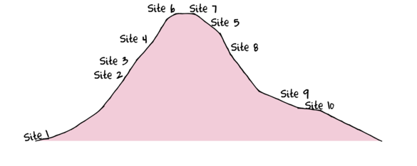
Multidimensional scaling

re-project objects (sites) in reduced dimensional space
must nominate the number of dimensions up-front
optimized patterns for the nominated dimensions

Q-mode analyses

	Sites	Sp1	Sp2	Sp3	Sp4	Sp5	Sp6	Sp7	Sp8	Sp9	Sp10
Site1	Site1	5	0	0	65	5	0	0	0	0	0
Site2	Site2	0	0	0	25	39	0	6	23	0	0
Site3	Site3	0	0	0	6	42	0	6	31	0	0
Site4	Site4	0	0	0	0	0	0	0	40	0	14
Site5	Site5	0	0	6	0	0	0	0	34	18	12
Site6	Site6	0	29	12	0	0	0	0	0	22	0
Site7	Site7	0	0	21	0	0	5	0	0	20	0
Site8	Site8	0	0	0	0	13	0	6	37	0	0
Site9	Site9	0	0	0	60	47	0	4	0	0	0
Site10	Site10	0	0	0	72	34	0	0	0	0	0

Multidimensional scaling

generate distance matrix

> data.dist <- vegdist(data[,-1], "bray")
> data.dist

           Site1     Site2     Site3     Site4     Site5     Site6     Site7     Site8     Site9
Site2  0.6428571                                                                                
Site3  0.8625000 0.1685393                                                                      
Site4  1.0000000 0.6870748 0.5539568                                                            
Site5  1.0000000 0.7177914 0.6000000 0.2580645                                                  
Site6  1.0000000 1.0000000 1.0000000 1.0000000 0.6390977                                        
Site7  1.0000000 1.0000000 1.0000000 1.0000000 0.5862069 0.4128440                              
Site8  0.9236641 0.4362416 0.2907801 0.3272727 0.4603175 1.0000000 1.0000000                    
Site9  0.3010753 0.3333333 0.4693878 1.0000000 1.0000000 1.0000000 1.0000000 0.7964072          
Site10 0.2265193 0.4070352 0.5811518 1.0000000 1.0000000 1.0000000 1.0000000 0.8395062 0.1336406

Multidimensional scaling

choose # dimensions (k=2)

Multidimensional scaling

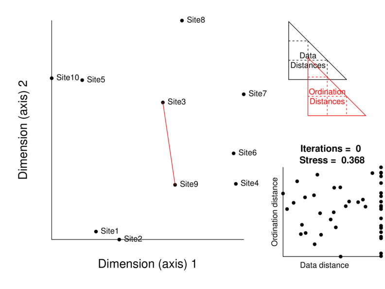
random configuration

Multidimensional scaling

measure Kruskal’s stress

Multidimensional scaling

iterate - gradient descent

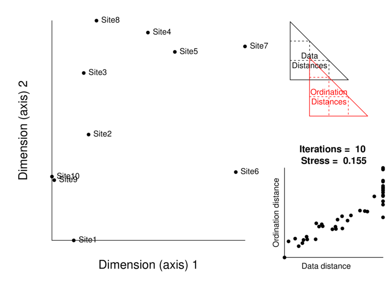
Multidimensional scaling

continual to iterate

Multidimensional scaling

continual (stopping criteria)

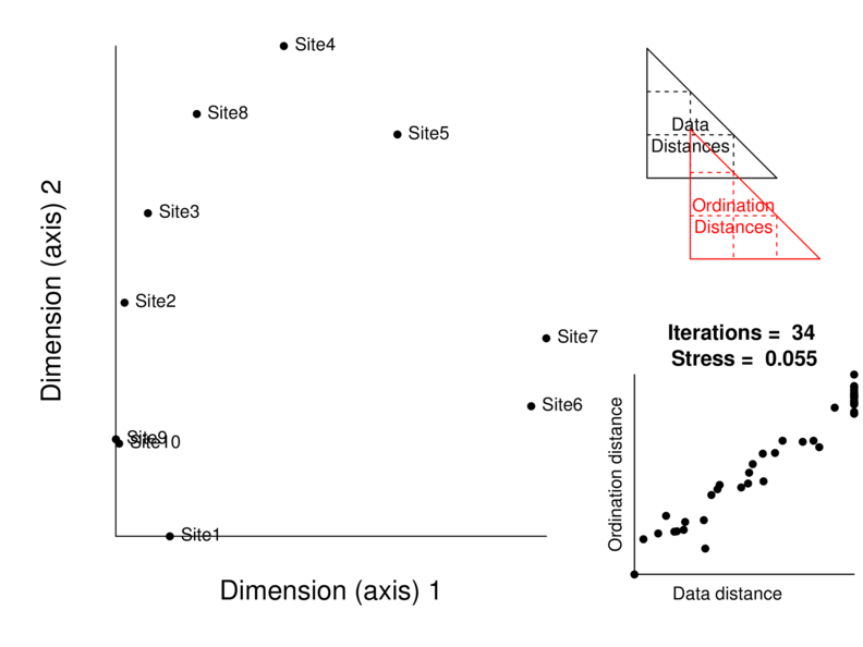
Multidimensional scaling

Stopping criteria

convergence tolerance (stress below a threshold)
the stress ratio (improvement in stress)
maximum iterations

Ideally stress < 0.2

Multidimensional scaling

Final configuration

axes have no real meaning
operate together to create ordination space
orientation of points is arbitrary

Multidimensional scaling

Starting contiguration

completely random
based on eigen-analysis
repeated random starts

Multidimensional scaling

Procrustes rotation

Multidimensional scaling

Procrustes rotation

Root mean square error (rmse)

rmse < 0.01, and no one > 0.005
stopping criteria

Multidimensional scaling

metaMDS()

transform and scale
generates dissimilarity
PCoA for starting config
up to 20 random starts
procrustes used to determine final config
final scores scaled
- PCA-like axes rotations

Multidimensional scaling

> library(vegan)
> data.nmds <- metaMDS(data[,-1])

Square root transformation
Wisconsin double standardization
Run 0 stress 9.575935e-05 
Run 1 stress 9.419141e-05 
... New best solution
... procrustes: rmse 0.02551179  max resid 0.04216078 
Run 2 stress 0.0005652599 
... procrustes: rmse 0.1885613  max resid 0.2962192 
Run 3 stress 0.0003846328 
... procrustes: rmse 0.128145  max resid 0.2569595 
Run 4 stress 0.1071568 
Run 5 stress 0.08642 
Run 6 stress 0.0002599177 
... procrustes: rmse 0.1766213  max resid 0.2933088 
Run 7 stress 9.39752e-05 
... New best solution
... procrustes: rmse 0.1050724  max resid 0.2432038 
Run 8 stress 9.692363e-05 
... procrustes: rmse 0.101578  max resid 0.2286374 
Run 9 stress 9.636878e-05 
... procrustes: rmse 0.03799946  max resid 0.06399347 
Run 10 stress 9.756922e-05 
... procrustes: rmse 0.09787159  max resid 0.2172152 
Run 11 stress 9.903768e-05 
... procrustes: rmse 0.1377402  max resid 0.2070494 
Run 12 stress 0.07877608 
Run 13 stress 9.67808e-05 
... procrustes: rmse 0.105466  max resid 0.2688797 
Run 14 stress 0.00122647 
Run 15 stress 0.002519856 
Run 16 stress 9.401245e-05 
... procrustes: rmse 0.01935187  max resid 0.04030324 
Run 17 stress 9.207175e-05 
... New best solution
... procrustes: rmse 0.1056994  max resid 0.2401655 
Run 18 stress 0.00139044 
Run 19 stress 9.781088e-05 
... procrustes: rmse 0.1089896  max resid 0.25471 
Run 20 stress 9.529673e-05 
... procrustes: rmse 0.09327002  max resid 0.1897497

Multidimensional scaling

> data.nmds


Call:
metaMDS(comm = data[, -1]) 

global Multidimensional Scaling using monoMDS

Data:     wisconsin(sqrt(data[, -1])) 
Distance: bray 

Dimensions: 2 
Stress:     9.207175e-05 
Stress type 1, weak ties
No convergent solutions - best solution after 20 tries
Scaling: centring, PC rotation, halfchange scaling 
Species: expanded scores based on 'wisconsin(sqrt(data[, -1]))'

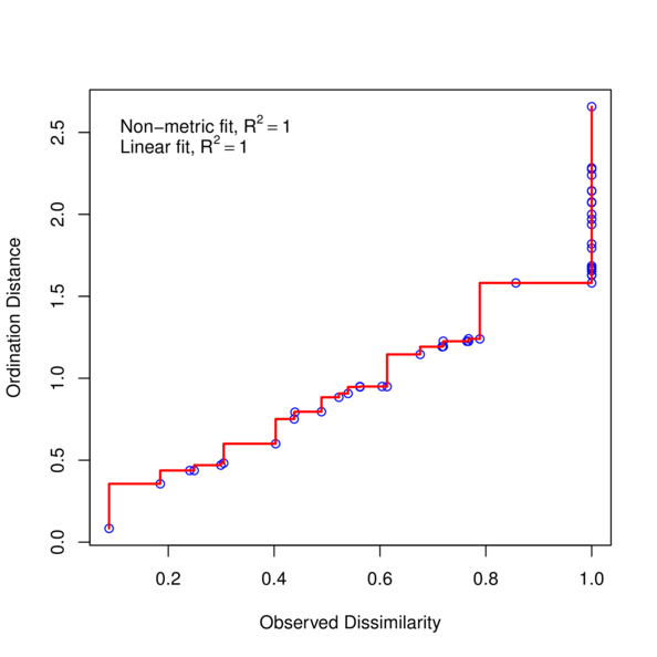
Multidimensional scaling

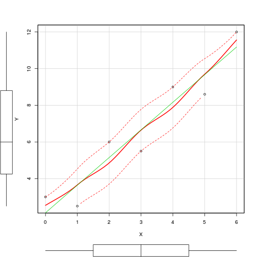
Shepard diagram

> stressplot(data.nmds)

Multidimensional scaling

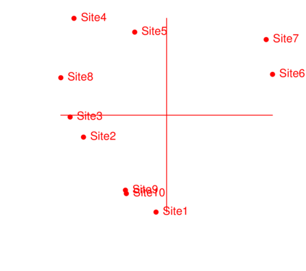
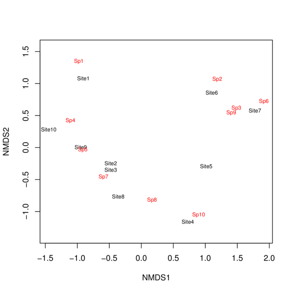
Ordination plot

> ordiplot(data.nmds, type="text")

Multidimensional scaling

Environmental fit

rotate axes to planes of maximum variability
observations are not independent
permutation tests - e.g based on \(R^2\)

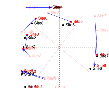
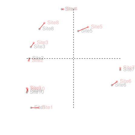
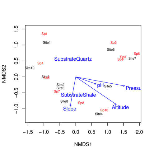
Multidimensional scaling

Environmental fit

> ordiplot(data.nmds, type="text")
> data.envfit <- envfit(data.nmds,enviro[,-1])
> plot(data.envfit)

Multidimensional scaling

Environmental fit

> data.envfit


***VECTORS

            NMDS1    NMDS2     r2 Pr(>r)   
pH        0.94416 -0.32948 0.1605  0.551   
Slope    -0.18315 -0.98308 0.3033  0.264   
Pressure  0.98333 -0.18182 0.8361  0.005 **
Altitude  0.82690 -0.56235 0.8107  0.002 **
---
Signif. codes:  0 '***' 0.001 '**' 0.01 '*' 0.05 '.' 0.1 ' ' 1
Permutation: free
Number of permutations: 999

***FACTORS:

Centroids:
                  NMDS1   NMDS2
SubstrateQuartz -0.0849  0.5622
SubstrateShale   0.0849 -0.5622

Goodness of fit:
              r2 Pr(>r)
Substrate 0.2178  0.144
Permutation: free
Number of permutations: 999

Q-mode Inference testing

Environmental correlates

	Sites	Sp1	Sp2	Sp3	Sp4	Sp5	Sp6	Sp7	Sp8	Sp9	Sp10
Site1	Site1	5	0	0	65	5	0	0	0	0	0
Site2	Site2	0	0	0	25	39	0	6	23	0	0
Site3	Site3	0	0	0	6	42	0	6	31	0	0
Site4	Site4	0	0	0	0	0	0	0	40	0	14
Site5	Site5	0	0	6	0	0	0	0	34	18	12
Site6	Site6	0	29	12	0	0	0	0	0	22	0
Site7	Site7	0	0	21	0	0	5	0	0	20	0
Site8	Site8	0	0	0	0	13	0	6	37	0	0
Site9	Site9	0	0	0	60	47	0	4	0	0	0
Site10	Site10	0	0	0	72	34	0	0	0	0	0

Environmental correlates

Site	pH	Slope	Pressure	Altitude	Substrate
Site1	6	4	101325	2	Quartz
Site2	7	9	101352	510	Shale
Site3	7	9	101356	546	Shale
Site4	7	7	101372	758	Shale
Site5	7	6	101384	813	Shale
Site6	8	8	101395	856	Quartz
Site7	8	0	101396	854	Quartz
Site8	7	12	101370	734	Shale
Site9	8	8	101347	360	Quartz
Site10	6	2	101345	356	Quartz

Environmental correlates

PCA/CA
- relate envir to first few axes
MDS with envfit
- relate envir to reduced optimized axes

All just relate envir to SOME patterns of community data

Mantel test

correlation of two distance matrices

Mantel test

Community distances

> library(vegan)
> data.dist <- vegdist(wisconsin(sqrt(data[,-1])),"bray")
> data.dist

            Site1      Site2      Site3      Site4      Site5      Site6
Site2  0.67587556                                                       
Site3  0.76402116 0.08814559                                            
Site4  1.00000000 0.76728722 0.71732569                                 
Site5  1.00000000 0.76728722 0.71950051 0.43782491                      
Site6  1.00000000 1.00000000 1.00000000 1.00000000 0.56217509           
Site7  1.00000000 1.00000000 1.00000000 1.00000000 0.56217509 0.40287938
Site8  0.85671371 0.24898448 0.18481903 0.61338910 0.71950051 1.00000000
Site9  0.52225127 0.24045299 0.30461844 1.00000000 1.00000000 1.00000000
Site10 0.43930743 0.53960530 0.60377075 1.00000000 1.00000000 1.00000000
            Site7      Site8      Site9
Site2                                  
Site3                                  
Site4                                  
Site5                                  
Site6                                  
Site7                                  
Site8  1.00000000                      
Site9  1.00000000 0.48943747           
Site10 1.00000000 0.78858978 0.29915230

Mantel test

Environmental distances

> library(vegan)
> enviro1 <- within(enviro,
+       Substrate<-as.numeric(Substrate))
> env.dist <- vegdist(decostand(enviro1[,-1],
+       "standardize"),"euclid")
> env.dist

           1         2         3         4         5         6         7
2  3.3229931                                                            
3  3.4352275 0.3112630                                                  
4  4.2003679 1.4095427 1.1199511                                        
5  4.6243094 2.1315293 1.8280978 0.7722349                              
6  4.9177360 3.1669299 2.9561936 2.3097932 2.1404251                    
7  4.9080429 4.0132037 3.7487386 3.0169364 2.5115880 2.2216568          
8  4.5387150 1.4066733 1.3097554 1.2431118 1.8378136 2.5328911 3.9603544
9  3.9400812 3.2272044 3.1427473 3.3444512 3.5238311 3.0372913 3.7500941
10 1.7177533 3.0391765 3.0117638 3.3462020 3.5745559 3.9177255 3.4387521
           8         9
2                     
3                     
4                     
5                     
6                     
7                     
8                     
9  3.4268548          
10 4.0495542 3.7782159

Mantel test

> plot(data.dist, env.dist)

Mantel test

> data.mantel <- mantel(data.dist, env.dist, perm=1000)
> data.mantel


Mantel statistic based on Pearson's product-moment correlation 

Call:
mantel(xdis = data.dist, ydis = env.dist, permutations = 1000) 

Mantel statistic r: 0.5593 
      Significance: 0.003996 

Upper quantiles of permutations (null model):
  90%   95% 97.5%   99% 
0.209 0.297 0.357 0.428 
Permutation: free
Number of permutations: 1000

Mantel test

> hist(data.mantel$perm)
> abline(v=data.mantel$statistic)

Best environmental subsets

looks at combinations of environmental predictors
analogous to model selection
not an inference test

Best environmental subsets

> # convert the Substrate factor to a numeric via dummy coding
> # function definition at the start of this Tutorial
> dummy <- function(x) {
+   nms <- colnames(x)
+   ff <- eval(parse(text=paste("~",paste(nms,collapse="+"))))
+   mm <- model.matrix(ff,x)
+   nms <- colnames(mm)
+   mm <- as.matrix(mm[,-1])
+   colnames(mm) <- nms[-1]
+   mm
+ }
> enviro1 <- dummy(enviro[,-1])
> enviro1

    pH Slope Pressure Altitude SubstrateShale
1  6.1   4.2   101325        2              0
2  6.7   9.2   101352      510              1
3  6.8   8.6   101356      546              1
4  7.0   7.4   101372      758              1
5  7.2   5.8   101384      813              1
6  7.5   8.4   101395      856              0
7  7.5   0.5   101396      854              0
8  7.0  11.8   101370      734              1
9  8.4   8.2   101347      360              0
10 6.2   1.5   101345      356              0

Best environmental subsets

> library(car)
> vif(lm(1:nrow(enviro1) ~ pH+Slope+Pressure+Altitude+SubstrateShale, data=data.frame(enviro1)))

            pH          Slope       Pressure 
      1.976424       2.187796      45.804821 
      Altitude SubstrateShale 
     52.754368       5.118418

> vif(lm(1:nrow(enviro1) ~ pH+Slope+Altitude+SubstrateShale, data=data.frame(enviro1)))

            pH          Slope       Altitude 
      1.968157       2.116732       1.830014 
SubstrateShale 
      2.636302

Best environmental subsets

> # Pressure is in column three
> data.bioenv <- bioenv(wisconsin(sqrt(data[,-1])), decostand(enviro1[,-3],"standardize"))
> data.bioenv


Call:
bioenv(comm = wisconsin(sqrt(data[, -1])), env = decostand(enviro1[,      -3], "standardize")) 

Subset of environmental variables with best correlation to community data.

Correlations:    spearman 
Dissimilarities: bray 
Metric:          euclidean 

Best model has 1 parameters (max. 4 allowed):
Altitude
with correlation  0.5514973

Permutation Multivariate Analysis of Variance

adonis

partitions the total sums of squares
- contribution of each predictor
permutation test of inference

Permutation Multivariate Analysis of Variance

adonis

> data.adonis <- adonis(data.dist ~ pH + Slope + Altitude + 
+    Substrate, data=enviro)
> data.adonis


Call:
adonis(formula = data.dist ~ pH + Slope + Altitude + Substrate,      data = enviro) 

Permutation: free
Number of permutations: 999

Terms added sequentially (first to last)

          Df SumsOfSqs MeanSqs F.Model      R2 Pr(>F)   
pH         1   0.21899 0.21899  1.6290 0.07768  0.209   
Slope      1   0.55960 0.55960  4.1628 0.19850  0.015 * 
Altitude   1   0.98433 0.98433  7.3223 0.34916  0.002 **
Substrate  1   0.38404 0.38404  2.8568 0.13623  0.057 . 
Residuals  5   0.67215 0.13443         0.23842          
Total      9   2.81911                 1.00000          
---
Signif. codes:  0 '***' 0.001 '**' 0.01 '*' 0.05 '.' 0.1 ' ' 1

Worked Examples

> data <- read.csv('../data/data.csv', strip.white=TRUE)
> head(data)

  Sites Sp1 Sp2 Sp3 Sp4 Sp5 Sp6 Sp7 Sp8 Sp9 Sp10
1 Site1   5   0   0  65   5   0   0   0   0    0
2 Site2   0   0   0  25  39   0   6  23   0    0
3 Site3   0   0   0   6  42   0   6  31   0    0
4 Site4   0   0   0   0   0   0   0  40   0   14
5 Site5   0   0   6   0   0   0   0  34  18   12
6 Site6   0  29  12   0   0   0   0   0  22    0

> enviro <- read.csv('../data/enviro.csv', strip.white=TRUE)
> head(enviro)

   Site  pH Slope Pressure Altitude Substrate
1 Site1 6.1   4.2   101325        2    Quartz
2 Site2 6.7   9.2   101352      510     Shale
3 Site3 6.8   8.6   101356      546     Shale
4 Site4 7.0   7.4   101372      758     Shale
5 Site5 7.2   5.8   101384      813     Shale
6 Site6 7.5   8.4   101395      856    Quartz

> data.bc <- vegdist(data[,-1], 'bray')
> 
> data.cpscale<-capscale(data.bc~ pH+Slope+Altitude+Substrate, data=enviro)
> plot(data.cpscale)

plot of chunk qmodeExamples

> str(data.cpscale)

List of 13
 $ call       : language capscale(formula = data.bc ~ pH + Slope + Altitude + Substrate, data = enviro)
 $ grand.total: logi NA
 $ rowsum     : logi NA
 $ colsum     : logi NA
 $ tot.chi    : num 2.76
 $ pCCA       : NULL
 $ CCA        :List of 12
  ..$ eig      : Named num [1:4] 1.266 0.978 0.073 0.03
  .. ..- attr(*, "names")= chr [1:4] "CAP1" "CAP2" "CAP3" "CAP4"
  ..$ u        : num [1:10, 1:4] -0.66766 -0.04799 -0.00444 0.24882 0.31907 ...
  .. ..- attr(*, "dimnames")=List of 2
  .. .. ..$ : chr [1:10] "1" "2" "3" "4" ...
  .. .. ..$ : chr [1:4] "CAP1" "CAP2" "CAP3" "CAP4"
  ..$ v        : num [1:6, 1:4] NA NA NA NA NA NA NA NA NA NA ...
  .. ..- attr(*, "dimnames")=List of 2
  .. .. ..$ : chr [1:6] "Dim1" "Dim2" "Dim3" "Dim4" ...
  .. .. ..$ : chr [1:4] "CAP1" "CAP2" "CAP3" "CAP4"
  ..$ wa       : num [1:10, 1:4] -0.4575 -0.1783 -0.0215 0.3049 0.4377 ...
  .. ..- attr(*, "dimnames")=List of 2
  .. .. ..$ : chr [1:10] "1" "2" "3" "4" ...
  .. .. ..$ : chr [1:4] "CAP1" "CAP2" "CAP3" "CAP4"
  ..$ biplot   : num [1:4, 1:4] 0.312 0.138 0.987 0.442 0.256 ...
  .. ..- attr(*, "dimnames")=List of 2
  .. .. ..$ : chr [1:4] "pH" "Slope" "Altitude" "SubstrateShale"
  .. .. ..$ : chr [1:4] "CAP1" "CAP2" "CAP3" "CAP4"
  ..$ rank     : int 4
  ..$ qrank    : int 4
  ..$ tot.chi  : num 2.35
  ..$ QR       :List of 4
  .. ..$ qr   : num [1:10, 1:4] 2.0159 0.1687 0.1191 0.0198 -0.0794 ...
  .. .. ..- attr(*, "dimnames")=List of 2
  .. .. .. ..$ : chr [1:10] "1" "2" "3" "4" ...
  .. .. .. ..$ : chr [1:4] "pH" "Slope" "Altitude" "SubstrateShale"
  .. ..$ rank : int 4
  .. ..$ qraux: num [1:4] 1.47 1.31 1.04 1.19
  .. ..$ pivot: int [1:4] 1 2 3 4
  .. ..- attr(*, "class")= chr "qr"
  ..$ envcentre: Named num [1:4] 7.04 6.56 578.9 0.5
  .. ..- attr(*, "names")= chr [1:4] "pH" "Slope" "Altitude" "SubstrateShale"
  ..$ Xbar     : num [1:10, 1:6] -1.261 -0.808 -0.401 0.787 1.424 ...
  .. ..- attr(*, "dimnames")=List of 2
  .. .. ..$ : chr [1:10] "1" "2" "3" "4" ...
  .. .. ..$ : chr [1:6] "Dim1" "Dim2" "Dim3" "Dim4" ...
  .. ..- attr(*, "scaled:center")= Named num [1:6] 1.80e-16 1.11e-16 -2.76e-16 7.79e-17 1.06e-15 ...
  .. .. ..- attr(*, "names")= chr [1:6] "Dim1" "Dim2" "Dim3" "Dim4" ...
  ..$ centroids: num [1:2, 1:4] -0.14 0.14 0.283 -0.283 0.015 ...
  .. ..- attr(*, "dimnames")=List of 2
  .. .. ..$ : chr [1:2] "SubstrateQuartz" "SubstrateShale"
  .. .. ..$ : chr [1:4] "CAP1" "CAP2" "CAP3" "CAP4"
 $ CA         :List of 9
  ..$ eig            : Named num [1:5] 0.35573 0.1688 0.04051 0.02265 0.00193
  .. ..- attr(*, "names")= chr [1:5] "MDS1" "MDS2" "MDS3" "MDS4" ...
  ..$ u              : num [1:10, 1:5] -0.567 0.262 0.28 -0.269 -0.342 ...
  .. ..- attr(*, "dimnames")=List of 2
  .. .. ..$ : chr [1:10] "1" "2" "3" "4" ...
  .. .. ..$ : chr [1:5] "MDS1" "MDS2" "MDS3" "MDS4" ...
  ..$ v              : num [1:6, 1:5] NA NA NA NA NA NA NA NA NA NA ...
  .. ..- attr(*, "dimnames")=List of 2
  .. .. ..$ : chr [1:6] "Dim1" "Dim2" "Dim3" "Dim4" ...
  .. .. ..$ : chr [1:5] "MDS1" "MDS2" "MDS3" "MDS4" ...
  ..$ rank           : int 5
  ..$ tot.chi        : num 0.59
  ..$ Xbar           : num [1:10, 1:6] 0.853 -0.373 -0.123 0.145 0.528 ...
  .. ..- attr(*, "dimnames")=List of 2
  .. .. ..$ : chr [1:10] "1" "2" "3" "4" ...
  .. .. ..$ : chr [1:6] "Dim1" "Dim2" "Dim3" "Dim4" ...
  .. ..- attr(*, "scaled:center")= Named num [1:6] 1.80e-16 1.11e-16 -2.76e-16 7.79e-17 1.06e-15 ...
  .. .. ..- attr(*, "names")= chr [1:6] "Dim1" "Dim2" "Dim3" "Dim4" ...
  ..$ imaginary.chi  : num -0.176
  ..$ imaginary.rank : int 3
  ..$ imaginary.u.eig: num [1:10, 1:3] -0.00467 -0.04869 0.01533 -0.00407 -0.01243 ...
  .. ..- attr(*, "dimnames")=List of 2
  .. .. ..$ : chr [1:10] "1" "2" "3" "4" ...
  .. .. ..$ : NULL
 $ method     : chr "capscale"
 $ inertia    : chr "squared Bray distance"
 $ terms      :Classes 'terms', 'formula' length 3 data.bc ~ pH + Slope + Altitude + Substrate
  .. ..- attr(*, "variables")= language list(data.bc, pH, Slope, Altitude, Substrate)
  .. ..- attr(*, "factors")= int [1:5, 1:4] 0 1 0 0 0 0 0 1 0 0 ...
  .. .. ..- attr(*, "dimnames")=List of 2
  .. .. .. ..$ : chr [1:5] "data.bc" "pH" "Slope" "Altitude" ...
  .. .. .. ..$ : chr [1:4] "pH" "Slope" "Altitude" "Substrate"
  .. ..- attr(*, "term.labels")= chr [1:4] "pH" "Slope" "Altitude" "Substrate"
  .. ..- attr(*, "specials")=Dotted pair list of 1
  .. .. ..$ Condition: NULL
  .. ..- attr(*, "order")= int [1:4] 1 1 1 1
  .. ..- attr(*, "intercept")= int 1
  .. ..- attr(*, "response")= int 1
  .. ..- attr(*, ".Environment")=<environment: R_GlobalEnv> 
 $ terminfo   :List of 3
  ..$ terms  :Classes 'terms', 'formula' length 2 ~pH + Slope + Altitude + Substrate
  .. .. ..- attr(*, "variables")= language list(pH, Slope, Altitude, Substrate)
  .. .. ..- attr(*, "factors")= int [1:4, 1:4] 1 0 0 0 0 1 0 0 0 0 ...
  .. .. .. ..- attr(*, "dimnames")=List of 2
  .. .. .. .. ..$ : chr [1:4] "pH" "Slope" "Altitude" "Substrate"
  .. .. .. .. ..$ : chr [1:4] "pH" "Slope" "Altitude" "Substrate"
  .. .. ..- attr(*, "term.labels")= chr [1:4] "pH" "Slope" "Altitude" "Substrate"
  .. .. ..- attr(*, "order")= int [1:4] 1 1 1 1
  .. .. ..- attr(*, "intercept")= int 1
  .. .. ..- attr(*, "response")= num 0
  .. .. ..- attr(*, ".Environment")=<environment: R_GlobalEnv> 
  ..$ xlev   :List of 1
  .. ..$ Substrate: chr [1:2] "Quartz" "Shale"
  ..$ ordered: Named logi [1:4] FALSE FALSE FALSE FALSE
  .. ..- attr(*, "names")= chr [1:4] "pH" "Slope" "Altitude" "Substrate"
 $ adjust     : num 3
 - attr(*, "class")= chr [1:3] "capscale" "rda" "cca"

> data.cmdscale <- cmdscale(data.bc, k=2)
> plot(data.cmdscale)

plot of chunk qmodeExamples

> data.scores <- scores(data.cmdscale)

Workshop 15: Q-mode MVA

Murray Logan

06 Aug 2016

R-mode analyses

Q-mode analyses

Dissimilarity

Distance measures

Distance measures

Distance measures

Multidimensional scaling

Q-mode analyses

Multidimensional scaling

Multidimensional scaling

Multidimensional scaling

Multidimensional scaling

Multidimensional scaling

Multidimensional scaling

Multidimensional scaling

Multidimensional scaling

Stopping criteria

Multidimensional scaling

Final configuration

Multidimensional scaling

Starting contiguration

Multidimensional scaling

Procrustes rotation

Multidimensional scaling

Procrustes rotation

Multidimensional scaling

Multidimensional scaling

Multidimensional scaling

Multidimensional scaling

Shepard diagram

Multidimensional scaling

Ordination plot

Multidimensional scaling

Environmental fit

Multidimensional scaling

Environmental fit

Multidimensional scaling

Environmental fit

Q-mode Inference testing

Environmental correlates

Environmental correlates

Environmental correlates

Permutation tests

Mantel test

Mantel test

Community distances

Mantel test

Environmental distances

Mantel test

Mantel test

Mantel test

Best environmental subsets

Best environmental subsets

Best environmental subsets

Best environmental subsets

Permutation Multivariate Analysis of Variance

adonis

Permutation Multivariate Analysis of Variance

adonis

Worked Examples

Worked Examples