Factorial ANOVA
- interactions
- \[y_{ijk} = \mu + \alpha_i + \beta_k + \alpha\beta_{ik} + \epsilon_{ijk}\]

| Factor | MS | F-ratio (both fixed) | F-ratio (A fixed, B random) | F-ratio (both random) |
|---|---|---|---|---|
| A | \(MS_A\) | \(MS_A/MS_{Resid}\) | \(MS_A/MS_{A:B}\) | \(MS_A/MS_{A:B}\) |
| B | \(MS_B\) | \(MS_B/MS_{Resid}\) | \(MS_B/MS_{Resid}\) | \(MS_B/MS_{A:B}\) |
| A:B | \(MS_{A:B}\) | \(MS_{A:B}/MS_{Resid}\) | \(MS_{A:B}/MS_{Resid}\) | \(MS_{A:B}/MS_{A:B}\) |
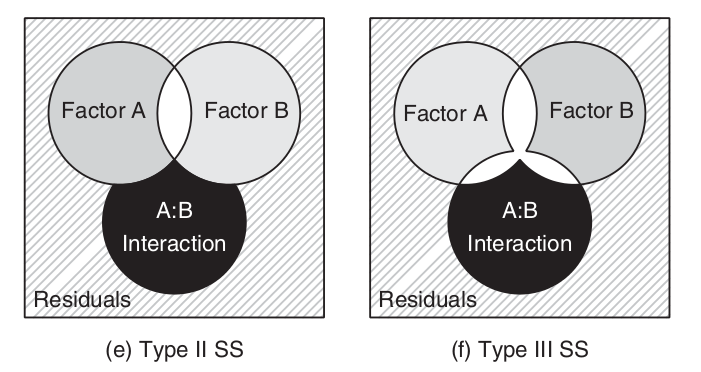
\[SS_{TOTAL} = SS_{A} + SS_{B} + SS_{A:B} + SS_{Resid}\]
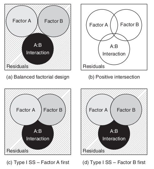
\[SS_{TOTAL} = SS_{A} + SS_{B} + SS_{A:B} + SS_{Resid}\]
\[SS_{TOTAL} \ne SS_{A} + SS_{B} + SS_{A:B} + SS_{Resid}\]
starling <- read.table("../data/starling.csv", header = T,
    sep = ",", strip.white = T)
head(starling)
SITUATION MONTH MASS GROUP
1 S1 November 78 S1Nov
2 S1 November 88 S1Nov
3 S1 November 87 S1Nov
4 S1 November 88 S1Nov
5 S1 November 83 S1Nov
6 S1 November 82 S1Nov
boxplot(MASS ~ SITUATION * MONTH, data = starling)

# Check for balance
replications(MASS ~ SITUATION * MONTH, data = starling)
SITUATION MONTH SITUATION:MONTH
20 40 10 !is.list(replications(MASS ~ SITUATION * MONTH, data = starling))[1] TRUE
starling.lm <- lm(MASS ~ SITUATION * MONTH, data = starling)
# setup a 2x6 plotting device with small margins
par(mfrow = c(2, 2), oma = c(0, 0, 2, 0))
plot(starling.lm, ask = F, which = 1:2)
plot(rstandard(starling.lm) ~ starling$SITUATION)
plot(rstandard(starling.lm) ~ starling$MONTH)

# Examine interaction plot - to help understand
# coefficients
library(car)
with(starling, interaction.plot(SITUATION, MONTH, MASS))

summary(starling.lm)
Call:
lm(formula = MASS ~ SITUATION * MONTH, data = starling)

Residuals:
   Min     1Q Median     3Q    Max
  -7.4   -3.2   -0.4    2.9    9.2

Coefficients:
                          Estimate Std. Error
(Intercept)                  90.80       1.33
SITUATIONS2                  -0.60       1.88
SITUATIONS3                  -2.60       1.88
SITUATIONS4                  -6.60       1.88
MONTHNovember                -7.20       1.88
SITUATIONS2:MONTHNovember    -3.60       2.66
SITUATIONS3:MONTHNovember    -2.40       2.66
SITUATIONS4:MONTHNovember    -1.60       2.66
                          t value Pr(>|t|)
(Intercept)                 68.26  < 2e-16 ***
SITUATIONS2                 -0.32  0.75069
SITUATIONS3                 -1.38  0.17121
SITUATIONS4                 -3.51  0.00078 ***
MONTHNovember               -3.83  0.00027 ***
SITUATIONS2:MONTHNovember   -1.35  0.18023
SITUATIONS3:MONTHNovember   -0.90  0.37000
SITUATIONS4:MONTHNovember   -0.60  0.54946
---
Signif. codes:  0 '***' 0.001 '**' 0.01 '*' 0.05 '.' 0.1 ' ' 1

Residual standard error: 4.21 on 72 degrees of freedom
Multiple R-squared:  0.64,  Adjusted R-squared:  0.605
F-statistic: 18.3 on 7 and 72 DF, p-value: 9.55e-14anova(starling.lm)Analysis of Variance Table
Response: MASS
Df Sum Sq Mean Sq F value Pr(>F)
SITUATION 3 574 191 10.82 6.0e-06
MONTH 1 1656 1656 93.60 1.2e-14
SITUATION:MONTH 3 34 11 0.64 0.59
Residuals 72 1274 18
SITUATION ***
MONTH ***
SITUATION:MONTH
Residuals
---
Signif. codes: 0 '***' 0.001 '**' 0.01 '*' 0.05 '.' 0.1 ' ' 1
library(multcomp)
summary(glht(starling.lm, linfct = mcp(SITUATION = "Tukey")))
     Simultaneous Tests for General Linear Hypotheses

Multiple Comparisons of Means: Tukey Contrasts


Fit: lm(formula = MASS ~ SITUATION * MONTH, data = starling)

Linear Hypotheses:
             Estimate Std. Error t value Pr(>|t|)
S2 - S1 == 0    -0.60       1.88   -0.32   0.9887
S3 - S1 == 0    -2.60       1.88   -1.38   0.5146
S4 - S1 == 0    -6.60       1.88   -3.51   0.0042
S3 - S2 == 0    -2.00       1.88   -1.06   0.7129
S4 - S2 == 0    -6.00       1.88   -3.19   0.0111
S4 - S3 == 0    -4.00       1.88   -2.13   0.1545

S2 - S1 == 0
S3 - S1 == 0
S4 - S1 == 0 **
S3 - S2 == 0
S4 - S2 == 0 *
S4 - S3 == 0
---
Signif. codes:  0 '***' 0.001 '**' 0.01 '*' 0.05 '.' 0.1 ' ' 1
(Adjusted p values reported -- single-step method)
# Added model
summary(glht(lm(MASS ~ SITUATION + MONTH, data = starling),
linfct = mcp(SITUATION = "Tukey")))
     Simultaneous Tests for General Linear Hypotheses

Multiple Comparisons of Means: Tukey Contrasts


Fit: lm(formula = MASS ~ SITUATION + MONTH, data = starling)

Linear Hypotheses:
             Estimate Std. Error t value Pr(>|t|)
S2 - S1 == 0    -2.40       1.32   -1.82   0.2734
S3 - S1 == 0    -3.80       1.32   -2.88   0.0261
S4 - S1 == 0    -7.40       1.32   -5.60   <0.001
S3 - S2 == 0    -1.40       1.32   -1.06   0.7147
S4 - S2 == 0    -5.00       1.32   -3.79   0.0018
S4 - S3 == 0    -3.60       1.32   -2.73   0.0389

S2 - S1 == 0
S3 - S1 == 0 *
S4 - S1 == 0 ***
S3 - S2 == 0
S4 - S2 == 0 **
S4 - S3 == 0 *
---
Signif. codes:  0 '***' 0.001 '**' 0.01 '*' 0.05 '.' 0.1 ' ' 1
(Adjusted p values reported -- single-step method)confint(glht(lm(MASS ~ SITUATION + MONTH, data = starling),
linfct = mcp(SITUATION = "Tukey")))
     Simultaneous Confidence Intervals

Multiple Comparisons of Means: Tukey Contrasts


Fit: lm(formula = MASS ~ SITUATION + MONTH, data = starling)

Quantile = 2.627
95% family-wise confidence level


Linear Hypotheses:
             Estimate lwr     upr
S2 - S1 == 0  -2.400   -5.870   1.070
S3 - S1 == 0  -3.800   -7.270  -0.330
S4 - S1 == 0  -7.400  -10.870  -3.930
S3 - S2 == 0  -1.400   -4.870   2.070
S4 - S2 == 0  -5.000   -8.470  -1.530
S4 - S3 == 0  -3.600   -7.070  -0.130
# Population means
library(effects)
starling.eff <- allEffects(starling.lm)
(starling.means <- with(starling.eff[[1]], data.frame(Fit = fit,
    Lower = lower, Upper = upper, x)))
Fit Lower Upper SITUATION MONTH
1 90.8 88.15 93.45 S1 January
2 90.2 87.55 92.85 S2 January
3 88.2 85.55 90.85 S3 January
4 84.2 81.55 86.85 S4 January
5 83.6 80.95 86.25 S1 November
6 79.4 76.75 82.05 S2 November
7 78.6 75.95 81.25 S3 November
8 75.4 72.75 78.05 S4 Novemberstarling.means <- starling.means[order(starling.means$SITUATION),
]
opar <- par(mar = c(5, 5, 1, 1))
xs <- barplot(starling.means$Fit, ylim = range(c(starling.means[,
2:3])), beside = T, axes = F, ann = F, axisnames = F,
xpd = F, axis.lty = 2, col = c(0, 1), space = c(1,
0, 1, 0, 1, 0))
arrows(xs, starling.means$Fit, xs, starling.means$Upper,
code = 2, length = 0.05, ang = 90)
axis(2, las = 1)
axis(1, at = apply(matrix(xs, nrow = 2), 2, median),
lab = c("Situation 1", "Situation 2", "Situation 3",
"Situation 4"))
mtext(2, text = "Mass (g) of starlings", line = 3,
cex = 1.25)
legend("topright", leg = c("January", "November"),
fill = c(0, 1), col = c(0, 1), bty = "n", cex = 1)
box(bty = "l")
par(opar)
# Raw data
opar <- par(mar = c(5, 5, 1, 1))
star.means <- with(starling, tapply(MASS, list(MONTH,
SITUATION), mean))
star.sds <- with(starling, tapply(MASS, list(MONTH,
SITUATION), sd))
star.len <- with(starling, tapply(MASS, list(MONTH,
SITUATION), length))
star.ses <- star.sds/sqrt(star.len)
xs <- barplot(star.means, ylim = range(starling$MASS),
beside = T, axes = F, ann = F, axisnames = F, xpd = F,
axis.lty = 2, col = c(0, 1))
arrows(xs, star.means, xs, star.means + star.ses, code = 2,
length = 0.05, ang = 90)
axis(2, las = 1)
axis(1, at = apply(xs, 2, median), lab = c("Situation 1",
"Situation 2", "Situation 3", "Situation 4"))
mtext(2, text = "Mass (g) of starlings", line = 3,
cex = 1.25)
legend("topright", leg = c("January", "November"),
fill = c(0, 1), col = c(0, 1), bty = "n", cex = 1)
box(bty = "l")
par(opar)
# Effect of month separately for each situtation
xmat <- expand.grid(SITUATION = levels(starling$SITUATION),
MONTH = levels(starling$MONTH))
mm <- model.matrix(~SITUATION * MONTH, xmat)
mm.jan <- mm[xmat$MONTH == "January", ]
mm.nov <- mm[xmat$MONTH == "November", ]
mm.sit <- mm.jan - mm.nov
data.frame(confint(glht(starling.lm, mm.sit))$confint,
Situation = xmat[xmat$MONTH == "January", 1]) Estimate lwr upr Situation
1 7.2 2.399 12.0 S1
2 10.8 5.999 15.6 S2
3 9.6 4.799 14.4 S3
4 8.8 3.999 13.6 S4# Worked examples
stehman <- read.table("../data/stehman.csv", header = T,
sep = ",", strip.white = T)
head(stehman) PH HEALTH GROUP BRATING
1 3 D D3 0.0
2 3 D D3 0.8
3 3 D D3 0.8
4 3 D D3 0.8
5 3 D D3 0.8
6 3 D D3 0.8
stehman$PH <- as.factor(stehman$PH)

boxplot(BRATING ~ HEALTH * PH, data = stehman)

replications(BRATING ~ HEALTH * PH, data = stehman)
$HEALTH
HEALTH
D H
67 28
$PH
PH
3 5.5 7
34 30 31
$`HEALTH:PH`
PH
HEALTH 3 5.5 7
D 23 23 21
H 11 7 10!is.list(replications(BRATING ~ HEALTH * PH, data = stehman))[1] FALSE
contrasts(stehman$HEALTH) <- contr.sum
contrasts(stehman$PH) <- contr.sum

stehman.lm <- lm(BRATING ~ HEALTH * PH, data = stehman)
par(mfrow = c(2, 2))
plot(stehman.lm, which = 1:2, ask = FALSE)
plot(rstandard(stehman.lm) ~ stehman$HEALTH)
plot(rstandard(stehman.lm) ~ stehman$PH)

library(car)
Anova(stehman.lm, type = "III")
Anova Table (Type III tests)
Response: BRATING
Sum Sq Df F value Pr(>F)
(Intercept) 114.1 1 444.87 <2e-16 ***
HEALTH 2.4 1 9.40 0.0029 **
PH 1.9 2 3.63 0.0306 *
HEALTH:PH 0.2 2 0.37 0.6897
Residuals 22.8 89
---
Signif. codes: 0 '***' 0.001 '**' 0.01 '*' 0.05 '.' 0.1 ' ' 1
library(car)
with(stehman, interaction.plot(PH, HEALTH, BRATING))

library(multcomp)
summary(glht(stehman.lm, linfct = mcp(PH = "Tukey")))
     Simultaneous Tests for General Linear Hypotheses

Multiple Comparisons of Means: Tukey Contrasts


Fit: lm(formula = BRATING ~ HEALTH * PH, data = stehman)

Linear Hypotheses:
             Estimate Std. Error t value Pr(>|t|)
5.5 - 3 == 0   -0.386      0.143   -2.69    0.023
7 - 3 == 0     -0.173      0.134   -1.29    0.407
7 - 5.5 == 0    0.213      0.146    1.46    0.316

5.5 - 3 == 0 *
7 - 3 == 0
7 - 5.5 == 0
---
Signif. codes:  0 '***' 0.001 '**' 0.01 '*' 0.05 '.' 0.1 ' ' 1
(Adjusted p values reported -- single-step method)
confint(glht(stehman.lm, linfct = mcp(PH = "Tukey")))
     Simultaneous Confidence Intervals

Multiple Comparisons of Means: Tukey Contrasts


Fit: lm(formula = BRATING ~ HEALTH * PH, data = stehman)

Quantile = 2.383
95% family-wise confidence level


Linear Hypotheses:
             Estimate lwr     upr
5.5 - 3 == 0 -0.3861  -0.7279 -0.0444
7 - 3 == 0   -0.1728  -0.4933  0.1476
7 - 5.5 == 0  0.2133  -0.1355  0.5620
stehman.lm2 <- lm(BRATING ~ PH * HEALTH, data = stehman,
    contrasts = list(PH = contr.poly(3, scores = c(3,
        5.5, 7)), HEALTH = contr.treatment))
summary(stehman.lm2)
Call:
lm(formula = BRATING ~ PH * HEALTH, data = stehman, contrasts = list(PH = contr.poly(3,
    scores = c(3, 5.5, 7)), HEALTH = contr.treatment))

Residuals:
    Min      1Q  Median      3Q     Max
-1.2286 -0.3238 -0.0087  0.3818  0.9913

Coefficients:
             Estimate Std. Error t value Pr(>|t|)
(Intercept)    1.0413     0.0619   16.81   <2e-16
PH.L          -0.0879     0.1077   -0.82   0.4162
PH.Q           0.2751     0.1069    2.57   0.0117
HEALTH2        0.3543     0.1155    3.07   0.0029
PH.L:HEALTH2  -0.1360     0.1899   -0.72   0.4758
PH.Q:HEALTH2  -0.1008     0.2099   -0.48   0.6323

(Intercept)  ***
PH.L
PH.Q         *
HEALTH2      **
PH.L:HEALTH2
PH.Q:HEALTH2
---
Signif. codes:  0 '***' 0.001 '**' 0.01 '*' 0.05 '.' 0.1 ' ' 1

Residual standard error: 0.506 on 89 degrees of freedom
Multiple R-squared:  0.196, Adjusted R-squared:  0.15
F-statistic: 4.33 on 5 and 89 DF, p-value: 0.00143confint(stehman.lm2) 2.5 % 97.5 %
(Intercept) 0.91821 1.1643
PH.L -0.30184 0.1260
PH.Q 0.06273 0.4875
HEALTH2 0.12475 0.5839
PH.L:HEALTH2 -0.51324 0.2413
PH.Q:HEALTH2 -0.51773 0.3162
# homogeneity of variance assumption TURNS OUT
# THAT THERE IS NO EVIDENCE OF NON-HOMOGENEITY
library(nlme)
stehman.gls <- gls(BRATING ~ HEALTH * PH, data = stehman)
stehman.gls1 <- gls(BRATING ~ HEALTH * PH, data = stehman,
    weights = varIdent(form = ~1 | HEALTH * PH))
anova(stehman.gls, stehman.gls1)
Model df AIC BIC logLik Test
stehman.gls 1 7 170.0 187.4 -78.0
stehman.gls1 2 12 175.6 205.5 -75.8 1 vs 2
L.Ratio p-value
stehman.gls
stehman.gls1 4.393 0.4944
anova(stehman.gls, type = "marginal")Denom. DF: 89
numDF F-value p-value
(Intercept) 1 444.9 <.0001
HEALTH 1 9.4 0.0029
PH 2 3.6 0.0306
HEALTH:PH 2 0.4 0.6897anova(stehman.gls1, type = "marginal")Denom. DF: 89
numDF F-value p-value
(Intercept) 1 341.4 <.0001
HEALTH 1 7.2 0.0086
PH 2 2.6 0.0809
HEALTH:PH 2 0.4 0.6545quinn <- read.table("../data/quinn.csv", header = T,
sep = ",", strip.white = T)
head(quinn) SEASON DENSITY RECRUITS SQRTRECRUITS GROUP
1 Spring Low 15 3.873 SpringLow
2 Spring Low 10 3.162 SpringLow
3 Spring Low 13 3.606 SpringLow
4 Spring Low 13 3.606 SpringLow
5 Spring Low 5 2.236 SpringLow
6 Spring High 11 3.317 SpringHigh
par(mfrow = c(1, 2))
boxplot(RECRUITS ~ SEASON * DENSITY, data = quinn)
boxplot(SQRTRECRUITS ~ SEASON * DENSITY, data = quinn)

!is.list(replications(sqrt(RECRUITS) ~ SEASON * DENSITY,
    data = quinn))
[1] FALSEreplications(sqrt(RECRUITS) ~ SEASON * DENSITY, data = quinn)$SEASON
SEASON
Autumn Spring Summer Winter
10 11 12 9
$DENSITY
DENSITY
High Low
24 18
$`SEASON:DENSITY`
DENSITY
SEASON High Low
Autumn 6 4
Spring 6 5
Summer 6 6
Winter 6 3contrasts(quinn$SEASON) <- contr.sum
contrasts(quinn$DENSITY) <- contr.sum
quinn.lm <- lm(SQRTRECRUITS ~ SEASON * DENSITY, data = quinn)
library(car)
Anova(quinn.lm, type = "III")Anova Table (Type III tests)
Response: SQRTRECRUITS
Sum Sq Df F value Pr(>F)
(Intercept) 540 1 529.04 < 2e-16 ***
SEASON 91 3 29.61 1.3e-09 ***
DENSITY 6 1 6.35 0.017 *
SEASON:DENSITY 11 3 3.71 0.021 *
Residuals 35 34
---
Signif. codes: 0 '***' 0.001 '**' 0.01 '*' 0.05 '.' 0.1 ' ' 1
library(car)
with(quinn, interaction.plot(SEASON, DENSITY, SQRTRECRUITS))
summary(quinn.lm)
Call:
lm(formula = SQRTRECRUITS ~ SEASON * DENSITY, data = quinn)

Residuals:
   Min     1Q Median     3Q    Max
-2.230 -0.598  0.138  0.549  1.886

Coefficients:
                 Estimate Std. Error t value
(Intercept)         3.692      0.161   23.00
SEASON1             0.552      0.281    1.97
SEASON2            -0.534      0.269   -1.98
SEASON3             2.067      0.261    7.91
DENSITY1            0.405      0.161    2.52
SEASON1:DENSITY1   -0.420      0.281   -1.49
SEASON2:DENSITY1   -0.543      0.269   -2.02
SEASON3:DENSITY1    0.702      0.261    2.69
                 Pr(>|t|)
(Intercept)       < 2e-16 ***
SEASON1             0.057 .
SEASON2             0.055 .
SEASON3           3.3e-09 ***
DENSITY1            0.017 *
SEASON1:DENSITY1    0.145
SEASON2:DENSITY1    0.052 .
SEASON3:DENSITY1    0.011 *
---
Signif. codes:  0 '***' 0.001 '**' 0.01 '*' 0.05 '.' 0.1 ' ' 1

Residual standard error: 1.01 on 34 degrees of freedom
Multiple R-squared:  0.753, Adjusted R-squared:  0.702
F-statistic: 14.8 on 7 and 34 DF,  p-value: 1.1e-08
library(biology)
AnovaM(quinn.lm.summer <- mainEffects(quinn.lm, at = SEASON ==
    "Summer"), type = "III")
Df Sum Sq Mean Sq F value Pr(>F)
INT 6 91.2 15.20 14.9 2.8e-08 ***
DENSITY 1 14.7 14.70 14.4 0.00058 ***
Residuals 34 34.7 1.02
---
Signif. codes: 0 '***' 0.001 '**' 0.01 '*' 0.05 '.' 0.1 ' ' 1library(biology)
AnovaM(quinn.lm. <- mainEffects(quinn.lm, at = SEASON ==
"Autumn"), type = "III") Df Sum Sq Mean Sq F value Pr(>F)
INT 6 105.9 17.65 17.3 4.7e-09 ***
DENSITY 1 0.0 0.00 0.0 0.96
Residuals 34 34.7 1.02
---
Signif. codes: 0 '***' 0.001 '**' 0.01 '*' 0.05 '.' 0.1 ' ' 1AnovaM(quinn.lm. <- mainEffects(quinn.lm, at = SEASON ==
"Winter"), type = "III") Df Sum Sq Mean Sq F value Pr(>F)
INT 6 102.4 17.06 16.72 7.1e-09 ***
DENSITY 1 3.5 3.54 3.47 0.071 .
Residuals 34 34.7 1.02
---
Signif. codes: 0 '***' 0.001 '**' 0.01 '*' 0.05 '.' 0.1 ' ' 1AnovaM(quinn.lm. <- mainEffects(quinn.lm, at = SEASON ==
"Spring"), type = "III") Df Sum Sq Mean Sq F value Pr(>F)
INT 6 105.7 17.61 17.3 4.8e-09 ***
DENSITY 1 0.2 0.21 0.2 0.65
Residuals 34 34.7 1.02
---
Signif. codes: 0 '***' 0.001 '**' 0.01 '*' 0.05 '.' 0.1 ' ' 1
# Or via contrasts - not this is still in sqrt
# scale which are not trivial to reverse (due to
# negatives)
library(contrast)
quinn.contr <- contrast(quinn.lm, a = list(SEASON = levels(quinn$SEASON),
    DENSITY = "High"), b = list(SEASON = levels(quinn$SEASON),
    DENSITY = "Low"))
with(quinn.contr, data.frame(SEASON, Contrast, Lower,
    Upper, testStat, df, Pvalue))
SEASON Contrast Lower Upper testStat df
1 Autumn -0.02996 -1.3550 1.2950 -0.04595 34
2 Spring -0.27653 -1.5195 0.9664 -0.45214 34
3 Summer 2.21340 1.0283 3.3985 3.79557 34
4 Winter 1.32959 -0.1219 2.7810 1.86162 34
Pvalue
1 0.9636151
2 0.6540421
3 0.0005794
4 0.0713198
# Or via contrasts
xmat <- with(quinn, expand.grid(SEASON = levels(SEASON),
    DENSITY = levels(DENSITY)))
contrasts(xmat$SEASON) <- "contr.sum"
contrasts(xmat$DENSITY) <- "contr.sum"
mm <- model.matrix(~SEASON * DENSITY, xmat)
mm.high <- mm[xmat$DENSITY == "High", ]
mm.low <- mm[xmat$DENSITY == "Low", ]
mm.density <- mm.high - mm.low
rownames(mm.density) <- levels(quinn$SEASON)
summary(glht(quinn.lm, mm.density))
     Simultaneous Tests for General Linear Hypotheses

Fit: lm(formula = SQRTRECRUITS ~ SEASON * DENSITY, data = quinn)

Linear Hypotheses:
            Estimate Std. Error t value Pr(>|t|)
Autumn == 0   -0.030      0.652   -0.05   1.0000
Spring == 0   -0.277      0.612   -0.45   0.9845
Summer == 0    2.213      0.583    3.80   0.0023
Winter == 0    1.330      0.714    1.86   0.2500

Autumn == 0
Spring == 0
Summer == 0 **
Winter == 0
---
Signif. codes:  0 '***' 0.001 '**' 0.01 '*' 0.05 '.' 0.1 ' ' 1
(Adjusted p values reported -- single-step method)data.frame(confint(glht(quinn.lm, mm.density))$confint,
SEASON = levels(quinn$SEASON)) Estimate lwr upr SEASON
Autumn -0.02996 -1.7399 1.680 Autumn
Spring -0.27653 -1.8806 1.328 Spring
Summer 2.21340 0.6839 3.743 Summer
Winter 1.32959 -0.5436 3.203 Winter