3
22.7
0.9
2.5
23.7
0.5
6
25.7
0.6
5.5
29.1
0.7
9
22
0.8
8.6
29
1.3
12
29.4
1
Multiple Linear Regression
Additive model
\[
\begin{alignat*}{1}
3~&=~\beta_0 ~&+~(\beta_1\times22.7) ~&+~(\beta_2\times0.9)~&+~\varepsilon_1\\
2.5~&=~\beta_0 ~&+~(\beta_1\times23.7) ~&+~(\beta_2\times0.5)~&+~\varepsilon_2\\
6~&=~\beta_0 ~&+~(\beta_1\times25.7) ~&+~(\beta_2\times0.6)~&+~\varepsilon_3\\
5.5~&=~\beta_0 ~&+~(\beta_1\times29.1) ~&+~(\beta_2\times0.7)~&+~\varepsilon_4\\
9~&=~\beta_0 ~&+~(\beta_1\times22) ~&+~(\beta_2\times0.8)~&+~\varepsilon_5\\
8.6~&=~\beta_0 ~&+~(\beta_1\times29) ~&+~(\beta_2\times1.3)~&+~\varepsilon_6\\
12~&=~\beta_0 ~&+~(\beta_1\times29.4) ~&+~(\beta_2\times1)~&+~\varepsilon_7\\
\end{alignat*}
\]
Multiple Linear Regression
Multiplicative model
\[growth = intercept + temp + nitro + temp\times nitro\]
\[y_i=\beta_0+\beta_1x_{i1}+\beta_2x_{i2}+\beta_3x_{i1}x_{i2}+...+\epsilon_i\]
Multiple Linear Regression
Multiplicative model
\[
\begin{alignat*}{1}
3~&=~\beta_0 ~&+~(\beta_1\times22.7) ~&+~(\beta_2\times0.9)~&+~(\beta_3\times22.7\times0.9)~&+~\varepsilon_1\\
2.5~&=~\beta_0 ~&+~(\beta_1\times23.7) ~&+~(\beta_2\times0.5)~&+~(\beta_3\times23.7\times0.5)~&+~\varepsilon_2\\
6~&=~\beta_0 ~&+~(\beta_1\times25.7) ~&+~(\beta_2\times0.6)~&+~(\beta_3\times25.7\times0.6)~&+~\varepsilon_3\\
5.5~&=~\beta_0 ~&+~(\beta_1\times29.1) ~&+~(\beta_2\times0.7)~&+~(\beta_3\times29.1\times0.7)~&+~\varepsilon_4\\
9~&=~\beta_0 ~&+~(\beta_1\times22) ~&+~(\beta_2\times0.8)~&+~(\beta_3\times22\times0.8)~&+~\varepsilon_5\\
8.6~&=~\beta_0 ~&+~(\beta_1\times29) ~&+~(\beta_2\times1.3)~&+~(\beta_3\times29\times1.3)~&+~\varepsilon_6\\
12~&=~\beta_0 ~&+~(\beta_1\times29.4) ~&+~(\beta_2\times1)~&+~(\beta_3\times29.4\times1)~&+~\varepsilon_7\\
\end{alignat*}
\]
Multiple Linear Regression
Centering
Multiple Linear Regression
Centering
Multiple Linear Regression
Centering
Multiple Linear Regression
Centering
Multiple Linear Regression
Centering
Multiple Linear Regression
Assumptions
Normality, homog., linearity
Multiple Linear Regression
Assumptions
(multi)collinearity
Multiple Linear Regression
Variance inflation
Strength of a relationship \[
R^2
\] Strong when \(R^2 \ge 0.8\)
Multiple Linear Regression
Variance inflation
\[
var.inf = \frac{1}{1-R^2}
\] Collinear when \(var.inf >= 5\)
Some prefer \(>3\)
Multiple Linear Regression
Assumptions
(multi)collinearity
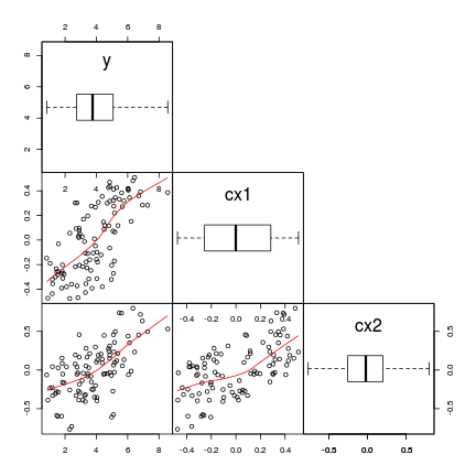
library (car)
# additive model - scaled predictors
vif (lm (y ~ cx1 + cx2, data)) cx1 cx2
1.743817 1.743817
Multiple Linear Regression
Assumptions
(multi)collinearity
library (car)
# additive model - scaled predictors
vif (lm (y ~ cx1 + cx2, data)) cx1 cx2
1.743817 1.743817 # multiplicative model - raw predictors
vif (lm (y ~ x1 * x2, data)) x1 x2 x1:x2
7.259729 5.913254 16.949468
Multiple Linear Regression
Assumptions
# multiplicative model - raw predictors
vif (lm (y ~ x1 * x2, data)) x1 x2 x1:x2
7.259729 5.913254 16.949468 # multiplicative model - scaled predictors
vif (lm (y ~ cx1 * cx2, data)) cx1 cx2 cx1:cx2
1.769411 1.771994 1.018694
Multiple linear models in R
Model fitting
Additive model
\(y_i=\beta_0+\beta_1x_{i1}+\beta_2x_{i2}+\epsilon_i\)
data.add.lm <- lm (y~cx1+cx2, data)
Model fitting
Additive model
\(y_i=\beta_0+\beta_1x_{i1}+\beta_2x_{i2}+\epsilon_i\)
data.add.lm <- lm (y~cx1+cx2, data)
\(y_i=\beta_0+\beta_1x_{i1}+\beta_2x_{i2}+\beta_3x_{i1}x_{i2}+\epsilon_i\)
data.mult.lm <- lm (y~cx1+cx2+cx1:cx2, data)
#OR
data.mult.lm <- lm (y~cx1*cx2, data)
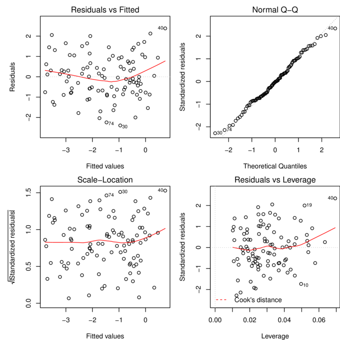
Model evaluation
Additive model
plot (data.add.lm)
Model evaluation
Multiplicative model
plot (data.mult.lm)
Model summary
Additive model
summary (data.add.lm)
Call:
lm(formula = y ~ cx1 + cx2, data = data)

Residuals:
     Min       1Q   Median       3Q      Max
-2.39418 -0.75888 -0.02463  0.73688  2.37938

Coefficients:
            Estimate Std. Error t value Pr(>|t|)
(Intercept)  -1.5161     0.1055 -14.364  < 2e-16 ***
cx1           2.5749     0.4683   5.499  3.1e-07 ***
cx2          -4.0475     0.3734 -10.839  < 2e-16 ***
---
Signif. codes:  0 '***' 0.001 '**' 0.01 '*' 0.05 '.' 0.1 ' ' 1

Residual standard error: 1.055 on 97 degrees of freedom
Multiple R-squared:  0.5567,    Adjusted R-squared:  0.5476
F-statistic: 60.91 on 2 and 97 DF,  p-value: < 2.2e-16
Model summary
Additive model
confint (data.add.lm) 2.5 % 97.5 %
(Intercept) -1.725529 -1.306576
cx1 1.645477 3.504300
cx2 -4.788628 -3.306308
Model summary
Multiplicative model
summary (data.mult.lm)
Call:
lm(formula = y ~ cx1 * cx2, data = data)

Residuals:
     Min       1Q   Median       3Q      Max
-2.23364 -0.62188  0.01763  0.80912  1.98568

Coefficients:
            Estimate Std. Error t value Pr(>|t|)
(Intercept)  -1.6995     0.1228 -13.836  < 2e-16 ***
cx1           2.7232     0.4571   5.957 4.22e-08 ***
cx2          -4.1716     0.3648 -11.435  < 2e-16 ***
cx1:cx2       2.5283     0.9373   2.697  0.00826 **
---
Signif. codes:  0 '***' 0.001 '**' 0.01 '*' 0.05 '.' 0.1 ' ' 1

Residual standard error: 1.023 on 96 degrees of freedom
Multiple R-squared:  0.588, Adjusted R-squared:  0.5751
F-statistic: 45.66 on 3 and 96 DF,  p-value: < 2.2e-16
Graphical summaries
Additive model
library (effects)
plot (effect ("cx1" ,data.add.lm, partial.residuals= TRUE ))
Graphical summaries
Additive model
library (effects)
library (ggplot2)
e <- effect ("cx1" ,data.add.lm, xlevels= list (
cx1= seq (-0.4 ,0.4 , len= 10 )), partial.residuals= TRUE )
newdata <- data.frame (fit= e$fit, cx1= e$x, lower= e$lower,
upper= e$upper)
resids <- data.frame (resid= e$partial.residuals.raw,
cx1= e$data$cx1) Error in data.frame(resid = e$partial.residuals.raw, cx1 = e$data$cx1): arguments imply differing number of rows: 0, 100ggplot (newdata, aes (y= fit, x= cx1)) +
geom_point (data= resids, aes (y= resid, x= cx1))+
geom_ribbon (aes (ymin= lower, ymax= upper), fill= 'blue' ,
alpha= 0.2 )+
geom_line ()+theme_classic ()Error in fortify(data): object 'resids' not found
Graphical summaries
Additive model
library (effects)
plot (allEffects (data.add.lm))
Graphical summaries
Multiplicative model
library (effects)
plot (allEffects (data.mult.lm))
Graphical summaries
Multiplicative model
library (effects)
plot (Effect (focal.predictors= c ("cx1" ,"cx2" ),data.mult.lm))
How good is a model?
“All models are wrong, but some are useful” George E. P. Box
Criteria
\(R^2\) - noInformation criteria
AIC, AICc
penalize for complexity
Model selection
Candidates
AIC (data.add.lm, data.mult.lm) df AIC
data.add.lm 4 299.5340
data.mult.lm 5 294.2283library (MuMIn)
AICc (data.add.lm, data.mult.lm) df AICc
data.add.lm 4 299.9551
data.mult.lm 5 294.8666
Model selection
Dredging
library (MuMIn)
data.mult.lm <- lm (y~cx1*cx2, data, na.action= na.fail)
dredge (data.mult.lm, rank= "AICc" , trace= TRUE )0 : lm(formula = y ~ 1, data = data, na.action = na.fail)
1 : lm(formula = y ~ cx1 + 1, data = data, na.action = na.fail)
2 : lm(formula = y ~ cx2 + 1, data = data, na.action = na.fail)
3 : lm(formula = y ~ cx1 + cx2 + 1, data = data, na.action = na.fail)
7 : lm(formula = y ~ cx1 + cx2 + cx1:cx2 + 1, data = data, na.action = na.fail)Global model call: lm(formula = y ~ cx1 * cx2, data = data, na.action = na.fail)
---
Model selection table
(Int) cx1 cx2 cx1:cx2 df logLik AICc delta weight
8 -1.699 2.7230 -4.172 2.528 5 -142.114 294.9 0.00 0.927
4 -1.516 2.5750 -4.047 4 -145.767 300.0 5.09 0.073
3 -1.516 -2.706 3 -159.333 324.9 30.05 0.000
1 -1.516 2 -186.446 377.0 82.15 0.000
2 -1.516 -0.7399 3 -185.441 377.1 82.27 0.000
Models ranked by AICc(x)
Multiple Linear Regression
Model averaging
library (MuMIn)
data.dredge<-dredge (data.mult.lm, rank= "AICc" )
model.avg (data.dredge, subset= delta<20 )
Call:
model.avg(object = data.dredge, subset = delta < 20)

Component models:
'123' '12'

Coefficients:
       (Intercept)      cx1       cx2  cx1:cx2
full     -1.686125 2.712397 -4.162525 2.344227
subset   -1.686125 2.712397 -4.162525 2.528328
Multiple Linear Regression
Model selection
Or more preferable:
identify 10-15 candidate models
compare these via AIC (etc)
Worked examples
Format of loyn.csv data file
ABUND
DIST
LDIST
AREA
GRAZE
ALT
YR.ISOL
..
..
..
..
..
..
..
ABUND
Abundance of forest birds in patch- response variable
DIST
Distance to nearest patch - predictor variable
LDIST
Distance to nearest larger patch - predictor variable
AREA
Size of the patch - predictor variable
GRAZE
Grazing intensity (1 to 5, representing light to heavy) - predictor variable
ALT
Altitude - predictor variable
YR.ISOL
Number of years since the patch was isolated - predictor variable
loyn <- read.csv ('../data/loyn.csv' , strip.white= T)
head (loyn) ABUND AREA YR.ISOL DIST LDIST GRAZE ALT
1 5.3 0.1 1968 39 39 2 160
2 2.0 0.5 1920 234 234 5 60
3 1.5 0.5 1900 104 311 5 140
4 17.1 1.0 1966 66 66 3 160
5 13.8 1.0 1918 246 246 5 140
6 14.1 1.0 1965 234 285 3 130
Worked Examples
Question: what effects do fragmentation variables have on the abundance of forest birds
Linear model:
\[
Abund_i = \beta_0 + \sum^N_{j=1:n}{\beta_j X_{ji}}+\varepsilon_i \hspace{1cm} \varepsilon \sim{} \mathcal{N}(0, \sigma^2)
\]