Workshop 9.15.4: Non-linearity
Murray Logan
10-11-2014
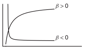
Linear models
\[
\begin{align*}
y_{i} &= \beta_0 + \beta_1 \times x_{i} + \varepsilon_i\\
\epsilon_i&\sim\mathcal{N}(0, \sigma^2) \\
\end{align*}
\]
Polynomials
LM
\(y \sim{} N(\mu, \sigma^2)\\ \mu = \beta_0 + \beta_1 x_1 + \beta_2 x_2\)
Polynomials
data.gp.lm <- lm (y~x+I (x^2 ), data= data.gp)
#OR
data.gp.lm <- lm (y~poly (x,2 ), data= data.gp)
summary (data.gp.lm)
Call:
lm(formula = y ~ poly(x, 2), data = data.gp)

Residuals:
       1        2        3        4        5
-0.00866  0.12987 -0.58009  0.57143 -0.11255

Coefficients:
             Estimate Std. Error t value Pr(>|t|)
(Intercept) -7.58e-17   2.63e-01    0.00     1.00
poly(x, 2)1  1.05e+00   5.88e-01    1.78     0.22
poly(x, 2)2 -2.87e+00   5.88e-01   -4.87     0.04

(Intercept)
poly(x, 2)1
poly(x, 2)2 *
---
Signif. codes:
0 '***' 0.001 '**' 0.01 '*' 0.05 '.' 0.1 ' ' 1

Residual standard error: 0.588 on 2 degrees of freedom
Multiple R-squared:  0.931, Adjusted R-squared:  0.861
F-statistic: 13.4 on 2 and 2 DF,  p-value: 0.0693
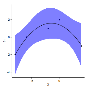
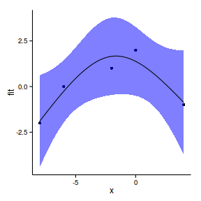
Polynomials
newdata <- data.frame (x= seq (min (data.gp$x),
max (data.gp$x), l= 100 ))
pred <- predict (data.gp.lm, newdata= newdata,
interval= 'confidence' )
newdata <- cbind (newdata,pred)
head (newdata) x fit lwr upr
1 -8.000 -1.991 -4.220 0.2376
2 -7.879 -1.859 -4.011 0.2922
3 -7.758 -1.730 -3.808 0.3483
4 -7.636 -1.603 -3.612 0.4061
5 -7.515 -1.478 -3.422 0.4655
6 -7.394 -1.356 -3.240 0.5268
Polynomials
ggplot (newdata, aes (y= fit, x= x))+
geom_point (data= data.gp, aes (y= y))+
geom_ribbon (aes (ymin= lwr,ymax= upr),fill= 'blue' ,alpha= 0.5 )+
geom_line ()+
theme_classic ()
Non-linear models
nls (y ~ a * exp (b*x), start= list (a= 1 , b= 1 ), data= data)
Non-linear models
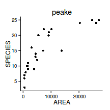
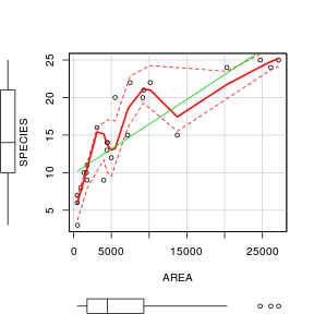
peake <- read.table ('../data/peake.csv' , header= T, sep= ',' , strip.white= T)
head (peake) AREA SPECIES INDIV
1 516.0 3 18
2 469.1 7 60
3 462.2 6 57
4 938.6 8 100
5 1357.2 10 48
6 1773.7 9 118library (car)
scatterplot (SPECIES~AREA,data= peake)
Non-linear models
Fit models
#Linear
peake.lmLin<-lm (SPECIES~AREA, data= peake)
#Polynomial
peake.lm <- lm (SPECIES~AREA+poly (AREA,2 ), data= peake)
#Power function
peake.nls <- nls (SPECIES~alpha*AREA^beta, data= peake,
start= list (alpha= 0.1 ,beta= 0.5 ))
#Assymptotic exponential
peake.nls.as <- nls (SPECIES~SSasymp (AREA,a,b,c),
data= peake)
Non-linear models
Model Validation
#Linear
plot (resid (peake.lmLin)~fitted (peake.lmLin))
Non-linear models
Model Validation
#calculate AIC for the linear model
AIC (peake.lmLin, peake.lm, peake.nls, peake.nls.as) df AIC
peake.lmLin 3 141.1
peake.lm 4 129.5
peake.nls 3 125.1
peake.nls.as 4 125.8#assess the goodness of fit between pairs of models
peake.nls1 <- peake.nls.as
anova (peake.lmLin,peake.lm)Analysis of Variance Table
Model 1: SPECIES ~ AREA
Model 2: SPECIES ~ AREA + poly(AREA, 2)
Res.Df RSS Df Sum of Sq F Pr(>F)
1 23 325
2 22 189 1 136 15.8 0.00064 ***
---
Signif. codes:
0 '***' 0.001 '**' 0.01 '*' 0.05 '.' 0.1 ' ' 1anova (peake.nls, peake.nls1)Analysis of Variance Table
Model 1: SPECIES ~ alpha * AREA^beta
Model 2: SPECIES ~ SSasymp(AREA, a, b, c)
Res.Df Res.Sum Sq Df Sum Sq F value Pr(>F)
1 23 172
2 22 163 1 9.14 1.24 0.28
Non-linear models
Model Validation
## calculate mean-square residual of the models
deviance (peake.lmLin)/df.residual (peake.lmLin)[1] 14.13deviance (peake.lm)/df.residual (peake.lm)[1] 8.602deviance (peake.nls)/df.residual (peake.nls)[1] 7.469deviance (peake.nls1)/df.residual (peake.nls1)[1] 7.393
Non-linear models
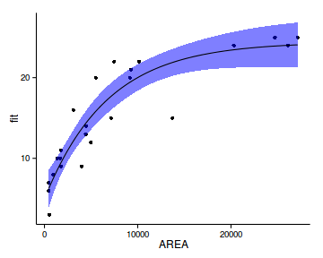
Plotting from SS models
xs<-with (peake,seq (min (AREA),max (AREA),l= 100 ))
ys <- predict (peake.nls.as, data.frame (AREA= xs))
se <- sqrt (apply (attr (ys,"gradient" ),1 ,function(x)
sum (vcov (peake.nls.as)*outer (x,x))))
newdata <- data.frame (AREA= xs, fit= ys,
lower= ys-2 *se,
upper= ys+2 *se)
head (newdata) AREA fit lower upper
1 462.2 6.248 3.907 8.589
2 731.8 6.962 4.866 9.057
3 1001.3 7.647 5.760 9.534
4 1270.8 8.305 6.590 10.021
5 1540.3 8.938 7.357 10.519
6 1809.8 9.546 8.065 11.026
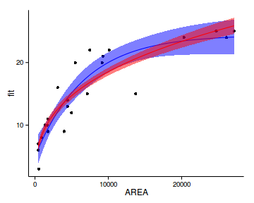
Non-linear models
Plotting from SS models
ggplot (newdata, aes (y= fit, x= AREA))+
geom_point (data= peake, aes (y= SPECIES))+
geom_ribbon (aes (ymin= lower,ymax= upper),
fill= 'blue' ,alpha= 0.5 )+
geom_line ()+
theme_classic ()
Non-linear models
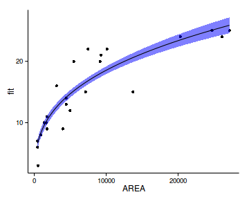
Plotting from own model
grad <- deriv3 (~alpha*AREA^beta, c ("alpha" ,"beta" ),
function(alpha,beta,AREA) NULL )
peake.nls<-nls (SPECIES~grad (alpha,beta,AREA),
data= peake,start= list (alpha= 0.1 ,beta= 1 ))
xs<-with (peake,seq (min (AREA),max (AREA),l= 100 ))
ys <- predict (peake.nls, data.frame (AREA= xs))
se.fit <- sqrt (apply (attr (ys,"gradient" ),1 ,function(x)
sum (vcov (peake.nls)*outer (x,x))))
newdata1 <- data.frame (AREA= xs, fit= ys, lower= ys-se.fit,
upper= ys+se.fit)
head (newdata1) AREA fit lower upper
1 462.2 6.648 5.908 7.388
2 731.8 7.749 7.004 8.494
3 1001.3 8.604 7.864 9.343
4 1270.8 9.316 8.586 10.046
5 1540.3 9.933 9.215 10.652
6 1809.8 10.482 9.776 11.189
Non-linear models
Plotting from SS models
ggplot (newdata1, aes (y= fit, x= AREA))+
geom_point (data= peake, aes (y= SPECIES))+
geom_ribbon (aes (ymin= lower,ymax= upper),
fill= 'blue' ,alpha= 0.5 )+
geom_line ()+
theme_classic ()
Non-linear models
Plotting both
ggplot (newdata, aes (y= fit, x= AREA))+
geom_point (data= peake, aes (y= SPECIES))+
geom_ribbon (aes (ymin= lower,ymax= upper),
fill= 'blue' ,alpha= 0.5 )+
geom_line (color= 'blue' )+
geom_ribbon (data= newdata1,aes (ymin= lower,ymax= upper),
fill= 'red' ,alpha= 0.5 )+
geom_line (data= newdata1,aes (y= fit,x= AREA), color= 'red' )+
theme_classic ()
Non-linear models
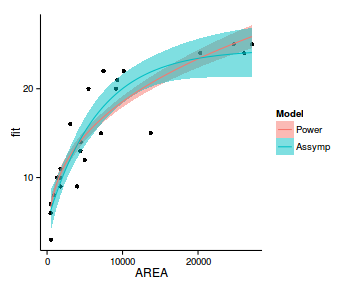
Plotting both
newdata2 <- rbind (cbind (Model= 'Power' ,newdata1),
cbind (Model= 'Assymp' ,newdata))
ggplot (data= newdata2, aes (y= fit, x= AREA))+
geom_point (data= peake, aes (y= SPECIES))+
geom_ribbon (aes (ymin= lower,ymax= upper, fill= Model),alpha= 0.5 )+
geom_line (aes (fill= Model, color= Model))+
theme_classic ()
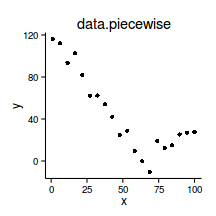
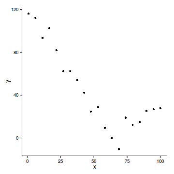
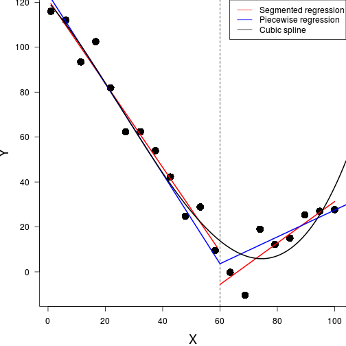
Piecewise Regression
data.piecewise <- read.csv ('../data/data.piecewise.csv' )
ggplot (data.piecewise, aes (y= y, x= x))+geom_point ()+
theme_classic ()
Piecewise Regression
Piecewise Regression
Piecewise Regression
\[
y_i=\beta_0 + \beta_1(x_i) + \beta_2(x_i > x_{cp})(x_i - cp)\\
\] \[
y_i=\beta_0 + \beta_1I(x_i < x_{cp})(x_i) + \beta_2I(x_i > x_{cp})(x_i - x_{cp})\\
\]
single knot
determined by hypothesis
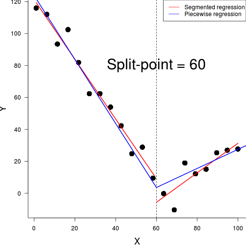
Piecewise Regression
#for a breakpoint of 60
data.piecewise.lm <- lm (y~x+I (ifelse (x>60 ,x-60 ,0 )),
data= data.piecewise)
summary (data.piecewise.lm)
Call:
lm(formula = y ~ x + I(ifelse(x > 60, x - 60, 0)), data = data.piecewise)

Residuals:
   Min     1Q Median     3Q    Max
-19.18  -3.79   1.28   3.96  11.99

Coefficients:
                             Estimate Std. Error
(Intercept)                   123.824      4.057
x                              -2.003      0.104
I(ifelse(x > 60, x - 60, 0))    2.600      0.239
                             t value Pr(>|t|)
(Intercept)                     30.5  2.7e-16 ***
x                              -19.3  5.5e-13 ***
I(ifelse(x > 60, x - 60, 0))    10.9  4.4e-09 ***
---
Signif. codes:
0 '***' 0.001 '**' 0.01 '*' 0.05 '.' 0.1 ' ' 1

Residual standard error: 7.61 on 17 degrees of freedom
Multiple R-squared:  0.965, Adjusted R-squared:  0.961
F-statistic:  233 on 2 and 17 DF,  p-value: 4.45e-13
Piecewise Regression
#for a breakpoint of 60
before <- function(x) ifelse (x<60 , 60 -x,0 )
after <- function(x) ifelse (x<60 , 0 , x-60 )
seq (0 ,100 ,by= 10 ) [1] 0 10 20 30 40 50 60 70 80 90 100before (seq (0 ,100 ,by= 10 )) [1] 60 50 40 30 20 10 0 0 0 0 0after (seq (0 ,100 ,by= 10 )) [1] 0 0 0 0 0 0 0 10 20 30 40before (70 )[1] 0data.piecewise.lm <- lm (y~before (x)+after (x), data= data.piecewise)
summary (data.piecewise.lm)
Call:
lm(formula = y ~ before(x) + after(x), data = data.piecewise)

Residuals:
   Min     1Q Median     3Q    Max
-19.18  -3.79   1.28   3.96  11.99

Coefficients:
            Estimate Std. Error t value Pr(>|t|)
(Intercept)    3.619      3.413    1.06   0.3038
before(x)      2.003      0.104   19.27  5.5e-13
after(x)       0.597      0.162    3.68   0.0018

(Intercept)
before(x)   ***
after(x)    **
---
Signif. codes:
0 '***' 0.001 '**' 0.01 '*' 0.05 '.' 0.1 ' ' 1

Residual standard error: 7.61 on 17 degrees of freedom
Multiple R-squared:  0.965, Adjusted R-squared:  0.961
F-statistic:  233 on 2 and 17 DF,  p-value: 4.45e-13
Piecewise Regression
#What if we dont know the breakpoint?
before <- function(x,bp) ifelse (x<bp, bp-x,0 )
after <- function(x,bp) ifelse (x<bp, 0 , x-bp)
piecewise <- function(bp) {
mod <- lm (y ~ before (x,bp)+after (x,bp),
data= data.piecewise)
sum (resid (mod)^2 )
}
search.range <- c (min (data.piecewise$x,na.rm= TRUE )+0.5 ,
max (data.piecewise$x, na.rm= TRUE )-0.5 )
search.range <- c (0 ,100 )
pw.opt <- optimize (piecewise, interval = search.range)
(bp <- pw.opt$minimum)[1] 65.51bp[1] 65.51mod <- lm (y ~ before (x,bp)+after (x,bp),
data= data.piecewise)
summary (mod)
Call:
lm(formula = y ~ before(x, bp) + after(x, bp), data = data.piecewise)

Residuals:
    Min      1Q  Median      3Q     Max
-11.549  -3.860   0.466   2.362  12.651

Coefficients:
              Estimate Std. Error t value
(Intercept)    -1.9740     2.9397   -0.67
before(x, bp)   1.8868     0.0809   23.31
after(x, bp)    0.9829     0.1657    5.93
              Pr(>|t|)
(Intercept)       0.51
before(x, bp)  2.4e-14 ***
after(x, bp)   1.6e-05 ***
---
Signif. codes:
0 '***' 0.001 '**' 0.01 '*' 0.05 '.' 0.1 ' ' 1

Residual standard error: 6.55 on 17 degrees of freedom
Multiple R-squared:  0.974, Adjusted R-squared:  0.971
F-statistic:  317 on 2 and 17 DF,  p-value: 3.48e-14
Linear models
only permit parametric non-linearity
polynomials
nls
piecewise regression
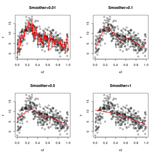
Cubic spline
Smoother
a function that relates Y to one or more X’s
types of smoothers
polynomials (parametric)
lowess, loess
splines
Smoother
non-parametric
no parameters
must be plotted to explore relationship
Smoother - lowess
Splines
library (splines)
ns (natural cubic splines)
bs (polynomial splines)
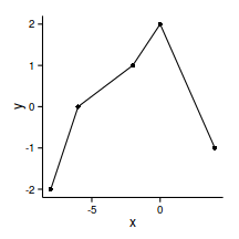
Splines
data.gp <- read.csv ('../data/data.gp.csv' )
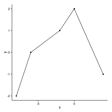
head (data.gp) x y
1 -8 -2
2 -6 0
3 -2 1
4 0 2
5 4 -1ggplot (data.gp, aes (y= y, x= x))+geom_point ()+geom_line ()+
theme_classic ()
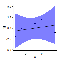
Splines
library (splines)
data.gp.lm <- lm (y~x, data= data.gp)
summary (data.gp.lm)
Call:
lm(formula = y ~ x, data = data.gp)

Residuals:
     1      2      3      4      5
-1.386  0.395  0.956  1.737 -1.702

Coefficients:
            Estimate Std. Error t value Pr(>|t|)
(Intercept)    0.263      0.884    0.30     0.79
x              0.110      0.180    0.61     0.59

Residual standard error: 1.72 on 3 degrees of freedom
Multiple R-squared:  0.11,  Adjusted R-squared:  -0.187
F-statistic: 0.369 on 1 and 3 DF,  p-value: 0.586
Splines
newdata <- data.frame (x= seq (min (data.gp$x),
max (data.gp$x), l= 100 ))
pred <- predict (data.gp.lm, newdata= newdata,interval= 'confidence' )
newdata <- cbind (newdata,pred)
ggplot (newdata, aes (y= fit, x= x))+
geom_point (data= data.gp, aes (y= y))+
geom_ribbon (aes (ymin= lwr,ymax= upr),fill= 'blue' ,alpha= 0.5 )+
geom_line ()+
theme_classic ()
Splines
library (splines)
ns (data.gp$x) 1
[1,] 0.0000
[2,] 0.1336
[3,] 0.4009
[4,] 0.5345
[5,] 0.8018
attr(,"degree")
[1] 3
attr(,"knots")
numeric(0)
attr(,"Boundary.knots")
[1] -8 4
attr(,"intercept")
[1] FALSE
attr(,"class")
[1] "ns" "basis" "matrix"ns (data.gp$x,k= 3 ) 1 2
[1,] 0.0000 0.0000
[2,] 0.1701 -0.1523
[3,] 0.4472 -0.2869
[4,] 0.5228 -0.1842
[5,] 0.4730 0.5634
attr(,"degree")
[1] 3
attr(,"knots")
[1] 3
attr(,"Boundary.knots")
[1] -8 4
attr(,"intercept")
[1] FALSE
attr(,"class")
[1] "ns" "basis" "matrix"ns (data.gp$x, df= 4 ) 1 2 3 4
[1,] 0.00000 0.0000 0.0000 0.00000
[2,] 0.08333 -0.1836 0.4590 -0.27541
[3,] 0.65000 0.2124 0.1357 -0.08145
[4,] 0.26667 0.5860 0.2018 -0.05439
[5,] 0.00000 -0.1579 0.3947 0.76316
attr(,"degree")
[1] 3
attr(,"knots")
25% 50% 75%
-6 -2 0
attr(,"Boundary.knots")
[1] -8 4
attr(,"intercept")
[1] FALSE
attr(,"class")
[1] "ns" "basis" "matrix"data.gp.lm <- lm (y~ns (x,df= 2 ), data= data.gp)
summary (data.gp.lm)
Call:
lm(formula = y ~ ns(x, df = 2), data = data.gp)

Residuals:
     1      2      3      4      5
-0.099  0.264 -0.657  0.622 -0.130

Coefficients:
               Estimate Std. Error t value
(Intercept)      -1.901      0.586   -3.24
ns(x, df = 2)1    5.815      1.427    4.07
ns(x, df = 2)2   -1.258      0.855   -1.47
               Pr(>|t|)
(Intercept)       0.083 .
ns(x, df = 2)1    0.055 .
ns(x, df = 2)2    0.279
---
Signif. codes:
0 '***' 0.001 '**' 0.01 '*' 0.05 '.' 0.1 ' ' 1

Residual standard error: 0.676 on 2 degrees of freedom
Multiple R-squared:  0.909, Adjusted R-squared:  0.817
F-statistic: 9.93 on 2 and 2 DF,  p-value: 0.0915
Splines
data.gp.ns <- lm (y~ns (x), data= data.gp)
summary (data.gp.ns)
Call:
lm(formula = y ~ ns(x), data = data.gp)

Residuals:
     1      2      3      4      5
-1.386  0.395  0.956  1.737 -1.702

Coefficients:
            Estimate Std. Error t value Pr(>|t|)
(Intercept)   -0.614      1.270   -0.48     0.66
ns(x)          1.641      2.700    0.61     0.59

Residual standard error: 1.72 on 3 degrees of freedom
Multiple R-squared:  0.11,  Adjusted R-squared:  -0.187
F-statistic: 0.369 on 1 and 3 DF,  p-value: 0.586
Splines
newdata <- data.frame (
x= seq (min (data.gp$x),
max (data.gp$x), l= 100 ))
pred <- predict (data.gp.lm, newdata= newdata,
interval= 'confidence' )
newdata <- cbind (newdata,pred)
head (newdata) x fit lwr upr
1 -8.000 -1.901 -4.423 0.6213
2 -7.879 -1.798 -4.248 0.6515
3 -7.758 -1.696 -4.075 0.6836
4 -7.636 -1.593 -3.905 0.7177
5 -7.515 -1.491 -3.737 0.7540
6 -7.394 -1.390 -3.572 0.7925newdata.ns <- newdata
pred.ns <- predict (data.gp.ns, newdata= newdata,
interval= 'confidence' )
newdata.ns <- cbind (newdata.ns,pred.ns)
head (newdata) x fit lwr upr
1 -8.000 -1.901 -4.423 0.6213
2 -7.879 -1.798 -4.248 0.6515
3 -7.758 -1.696 -4.075 0.6836
4 -7.636 -1.593 -3.905 0.7177
5 -7.515 -1.491 -3.737 0.7540
6 -7.394 -1.390 -3.572 0.7925
Splines
ggplot (newdata, aes (y= fit, x= x))+
geom_point (data= data.gp, aes (y= y))+
geom_ribbon (aes (ymin= lwr,ymax= upr),fill= 'blue' ,alpha= 0.5 )+
geom_line ()+
theme_classic ()
ggplot (newdata.ns, aes (y= fit, x= x))+
geom_point (data= data.gp, aes (y= y))+
geom_ribbon (aes (ymin= lwr,ymax= upr),fill= 'blue' ,alpha= 0.5 )+
geom_line ()+
theme_classic ()
Splines
data.gp.ns1 <- lm (y~ns (x,k= 1 ), data= data.gp)
summary (data.gp.ns1)
Call:
lm(formula = y ~ ns(x, k = 1), data = data.gp)

Residuals:
      1       2       3       4       5
-0.1720  0.3791 -0.5652  0.4162 -0.0581

Coefficients:
              Estimate Std. Error t value
(Intercept)     -1.828      0.492   -3.72
ns(x, k = 1)1    5.587      1.245    4.49
ns(x, k = 1)2   -2.183      0.778   -2.81
              Pr(>|t|)
(Intercept)      0.065 .
ns(x, k = 1)1    0.046 *
ns(x, k = 1)2    0.107
---
Signif. codes:
0 '***' 0.001 '**' 0.01 '*' 0.05 '.' 0.1 ' ' 1

Residual standard error: 0.579 on 2 degrees of freedom
Multiple R-squared:  0.933, Adjusted R-squared:  0.866
F-statistic: 13.9 on 2 and 2 DF,  p-value: 0.0669
Splines
newdata1 <- data.frame (
x= seq (min (data.gp$x),
max (data.gp$x), l= 100 ))
pred1 <- predict (data.gp.ns1, newdata= newdata1,
interval= 'confidence' )
newdata1 <- cbind (newdata1,pred1)
head (newdata1) x fit lwr upr
1 -8.000 -1.828 -3.944 0.2883
2 -7.879 -1.738 -3.800 0.3241
3 -7.758 -1.648 -3.656 0.3611
4 -7.636 -1.558 -3.515 0.3994
5 -7.515 -1.468 -3.374 0.4390
6 -7.394 -1.378 -3.236 0.4801
Splines
ggplot (newdata1, aes (y= fit, x= x))+
geom_point (data= data.gp, aes (y= y))+
geom_ribbon (aes (ymin= lwr,ymax= upr),fill= 'blue' ,alpha= 0.5 )+
geom_line ()+
theme_classic ()
Splines
anova (data.gp.lm,data.gp.ns, data.gp.ns1)Analysis of Variance Table
Model 1: y ~ ns(x, df = 2)
Model 2: y ~ ns(x)
Model 3: y ~ ns(x, k = 1)
Res.Df RSS Df Sum of Sq F Pr(>F)
1 2 0.91
2 3 8.90 -1 -7.99 17.5 0.053 .
3 2 0.67 1 8.23 18.0 0.051 .
---
Signif. codes:
0 '***' 0.001 '**' 0.01 '*' 0.05 '.' 0.1 ' ' 1AIC (data.gp.lm, data.gp.ns, data.gp.ns1) df AIC
data.gp.lm 4 13.70
data.gp.ns 3 23.07
data.gp.ns1 4 12.14
Splines
library (splines)
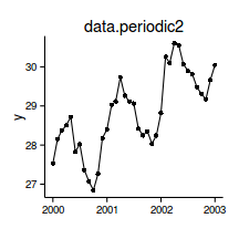
data.periodic2 <- read.csv ('../data/data.periodic2.csv' )
head (data.periodic2) y time month day
1 27.53 2000-01-01 1 0.002807
2 28.15 2000-02-01 2 0.089825
3 28.37 2000-03-01 3 0.171228
4 28.51 2000-04-01 4 0.258246
5 28.72 2000-05-01 5 0.342456
6 27.83 2000-06-01 6 0.429474library (lubridate)
data.periodic2$Dt.num <- decimal_date (as.Date (data.periodic2$time))
data.periodic2.ns <- lm (y~ns (Dt.num), data= data.periodic2)
summary (data.periodic2.ns)
Call:
lm(formula = y ~ ns(Dt.num), data = data.periodic2)

Residuals:
    Min      1Q  Median      3Q     Max
-1.3889 -0.5069 -0.0134  0.5559  1.1787

Coefficients:
            Estimate Std. Error t value Pr(>|t|)
(Intercept)   27.645      0.227  121.67  < 2e-16
ns(Dt.num)     2.959      0.488    6.06  6.4e-07

(Intercept) ***
ns(Dt.num)  ***
---
Signif. codes:
0 '***' 0.001 '**' 0.01 '*' 0.05 '.' 0.1 ' ' 1

Residual standard error: 0.706 on 35 degrees of freedom
Multiple R-squared:  0.512, Adjusted R-squared:  0.498
F-statistic: 36.8 on 1 and 35 DF,  p-value: 6.35e-07
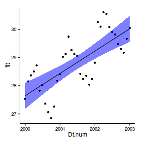
Splines
newdata <- data.frame (
Dt.num= seq (min (data.periodic2$Dt.num),
max (data.periodic2$Dt.num), l= 100 ))
pred <- predict (data.periodic2.ns, newdata= newdata,
interval= 'confidence' )
newdata <- cbind (newdata,pred)
head (newdata) Dt.num fit lwr upr
1 2000 27.64 27.18 28.11
2 2000 27.67 27.21 28.12
3 2000 27.69 27.24 28.14
4 2000 27.72 27.28 28.16
5 2000 27.74 27.31 28.17
6 2000 27.76 27.34 28.19
Splines
ggplot (newdata, aes (y= fit, x= Dt.num))+
geom_point (data= data.periodic2, aes (y= y))+
geom_ribbon (aes (ymin= lwr,ymax= upr),fill= 'blue' ,alpha= 0.5 )+
geom_line ()+
theme_classic ()
Splines
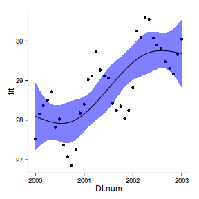
data.periodic2.ns <- lm (y~ns (Dt.num,df= 4 ), data= data.periodic2)
summary (data.periodic2.ns)
Call:
lm(formula = y ~ ns(Dt.num, df = 4), data = data.periodic2)

Residuals:
   Min     1Q Median     3Q    Max
-1.224 -0.556  0.103  0.488  1.289

Coefficients:
                    Estimate Std. Error t value
(Intercept)           28.097      0.424   66.27
ns(Dt.num, df = 4)1    0.699      0.567    1.23
ns(Dt.num, df = 4)2    1.889      0.554    3.41
ns(Dt.num, df = 4)3    1.340      1.095    1.22
ns(Dt.num, df = 4)4    1.799      0.512    3.51
                    Pr(>|t|)
(Intercept)           <2e-16 ***
ns(Dt.num, df = 4)1   0.2265
ns(Dt.num, df = 4)2   0.0018 **
ns(Dt.num, df = 4)3   0.2303
ns(Dt.num, df = 4)4   0.0013 **
---
Signif. codes:
0 '***' 0.001 '**' 0.01 '*' 0.05 '.' 0.1 ' ' 1

Residual standard error: 0.702 on 32 degrees of freedom
Multiple R-squared:  0.558, Adjusted R-squared:  0.503
F-statistic: 10.1 on 4 and 32 DF,  p-value: 2.07e-05
Splines
newdata <- data.frame (Dt.num= seq (min (data.periodic2$Dt.num), max (data.periodic2$Dt.num), l= 100 ))
pred <- predict (data.periodic2.ns, newdata= newdata, interval= 'confidence' )
newdata <- cbind (newdata,pred)
head (newdata) Dt.num fit lwr upr
1 2000 28.10 27.23 28.96
2 2000 28.08 27.27 28.89
3 2000 28.07 27.31 28.82
4 2000 28.05 27.35 28.76
5 2000 28.04 27.38 28.69
6 2000 28.02 27.41 28.64
Splines
ggplot (newdata, aes (y= fit, x= Dt.num))+
geom_point (data= data.periodic2, aes (y= y))+
geom_ribbon (aes (ymin= lwr,ymax= upr),fill= 'blue' ,alpha= 0.5 )+
geom_line ()+
theme_classic ()
Splines
data.periodic2.ns <- lm (y~ns (Dt.num,df= 7 ), data= data.periodic2)
summary (data.periodic2.ns)
Call:
lm(formula = y ~ ns(Dt.num, df = 7), data = data.periodic2)

Residuals:
    Min      1Q  Median      3Q     Max
-0.5270 -0.2335  0.0417  0.2266  0.5712

Coefficients:
                    Estimate Std. Error t value
(Intercept)           27.893      0.241  115.62
ns(Dt.num, df = 7)1   -1.980      0.344   -5.76
ns(Dt.num, df = 7)2    3.720      0.422    8.81
ns(Dt.num, df = 7)3   -1.815      0.385   -4.72
ns(Dt.num, df = 7)4    3.513      0.400    8.78
ns(Dt.num, df = 7)5    1.105      0.333    3.32
ns(Dt.num, df = 7)6    2.401      0.623    3.86
ns(Dt.num, df = 7)7    1.359      0.281    4.83
                    Pr(>|t|)
(Intercept)          < 2e-16 ***
ns(Dt.num, df = 7)1  3.1e-06 ***
ns(Dt.num, df = 7)2  1.1e-09 ***
ns(Dt.num, df = 7)3  5.5e-05 ***
ns(Dt.num, df = 7)4  1.2e-09 ***
ns(Dt.num, df = 7)5  0.00242 **
ns(Dt.num, df = 7)6  0.00059 ***
ns(Dt.num, df = 7)7  4.0e-05 ***
---
Signif. codes:
0 '***' 0.001 '**' 0.01 '*' 0.05 '.' 0.1 ' ' 1

Residual standard error: 0.325 on 29 degrees of freedom
Multiple R-squared:  0.915, Adjusted R-squared:  0.894
F-statistic: 44.3 on 7 and 29 DF,  p-value: 8.44e-14
Splines
newdata <- data.frame (Dt.num= seq (min (data.periodic2$Dt.num), max (data.periodic2$Dt.num), l= 100 ))
pred <- predict (data.periodic2.ns, newdata= newdata, interval= 'confidence' )
newdata <- cbind (newdata,pred)
head (newdata) Dt.num fit lwr upr
1 2000 27.89 27.40 28.39
2 2000 27.95 27.51 28.39
3 2000 28.01 27.62 28.40
4 2000 28.07 27.72 28.42
5 2000 28.12 27.81 28.43
6 2000 28.17 27.88 28.45
Splines
ggplot (newdata, aes (y= fit, x= Dt.num))+
geom_point (data= data.periodic2, aes (y= y))+
geom_ribbon (aes (ymin= lwr,ymax= upr),fill= 'blue' ,alpha= 0.5 )+
geom_line ()+
theme_classic ()
Splines
data.periodic2.ns <- lm (y~ns (Dt.num,df= 2 ) + ns (month,df= 3 ), data= data.periodic2)
summary (data.periodic2.ns)
Call:
lm(formula = y ~ ns(Dt.num, df = 2) + ns(month, df = 3), data = data.periodic2)

Residuals:
    Min      1Q  Median      3Q     Max
-0.4370 -0.2057  0.0185  0.1677  0.6720

Coefficients:
                    Estimate Std. Error t value
(Intercept)           27.363      0.150  182.14
ns(Dt.num, df = 2)1    3.268      0.276   11.82
ns(Dt.num, df = 2)2    2.354      0.151   15.63
ns(month, df = 3)1    -1.453      0.188   -7.73
ns(month, df = 3)2     0.772      0.298    2.59
ns(month, df = 3)3    -1.679      0.139  -12.07
                    Pr(>|t|)
(Intercept)          < 2e-16 ***
ns(Dt.num, df = 2)1  5.1e-13 ***
ns(Dt.num, df = 2)2  3.0e-16 ***
ns(month, df = 3)1   1.0e-08 ***
ns(month, df = 3)2     0.014 *
ns(month, df = 3)3   3.0e-13 ***
---
Signif. codes:
0 '***' 0.001 '**' 0.01 '*' 0.05 '.' 0.1 ' ' 1

Residual standard error: 0.266 on 31 degrees of freedom
Multiple R-squared:  0.939, Adjusted R-squared:  0.929
F-statistic: 95.1 on 5 and 31 DF,  p-value: <2e-16
Splines
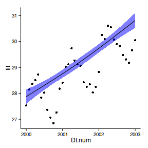
Long-term trend
newdata <- data.frame (
Dt.num= seq (min (data.periodic2$Dt.num), max (data.periodic2$Dt.num), l= 100 ),
month= 6 )
pred <- predict (data.periodic2.ns, newdata= newdata, interval= 'confidence' )
newdata <- cbind (newdata,pred)
head (newdata) Dt.num month fit lwr upr
1 2000 6 27.87 27.60 28.15
2 2000 6 27.90 27.63 28.17
3 2000 6 27.93 27.67 28.19
4 2000 6 27.95 27.70 28.21
5 2000 6 27.98 27.73 28.22
6 2000 6 28.00 27.77 28.24
Splines
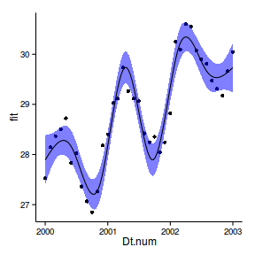
ggplot (newdata, aes (y= fit, x= Dt.num))+
geom_point (data= data.periodic2, aes (y= y))+
geom_ribbon (aes (ymin= lwr,ymax= upr),fill= 'blue' ,alpha= 0.5 )+
geom_line ()+
theme_classic ()
Splines
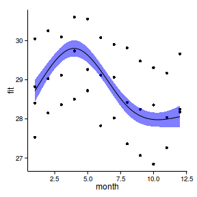
Long-term trend
newdata <- data.frame (
month= seq (1 ,12 , l= 100 ),
Dt.num= 2001.5 )
pred <- predict (data.periodic2.ns, newdata= newdata, interval= 'confidence' )
newdata <- cbind (newdata,pred)
head (newdata) month Dt.num fit lwr upr
1 1.000 2002 28.72 28.44 29.00
2 1.111 2002 28.78 28.51 29.05
3 1.222 2002 28.84 28.58 29.10
4 1.333 2002 28.90 28.65 29.15
5 1.444 2002 28.96 28.72 29.20
6 1.556 2002 29.02 28.79 29.25
Splines
ggplot (newdata, aes (y= fit, x= month))+
geom_point (data= data.periodic2, aes (y= y))+
geom_ribbon (aes (ymin= lwr,ymax= upr),fill= 'blue' ,alpha= 0.5 )+
geom_line ()+
theme_classic ()
Splines
Issues
Number of knots (df)
How to arrange the knots
evenly (cubic spline) - ns
density dependent - ps
Large datasets
thin-plate
fewer coefficients (low rank)
Degree of smoothing
\(\lambda\)
compromise
under and over smoothing
describe trend without focusing on outliers
model fit (residual sum of squares)
penalized for degree of smoothing (wiggliness)
Degree of smoothing
Generalized Cross-validation
create as many subsets as their are observations
fit all models with all \(\lambda\)
select best \(\lambda\)
Generalized Additive Models
LM
\(y \sim{} N(\mu, \sigma^2)\\ \mu = \beta_0 + \beta_1 x_1 + \beta_2 x_2\)
GLM
\(y \sim{} Pois(\mu, \sigma^2)\\ g(\mu) = \beta_0 + \beta_1 x_1 + \beta_2 x_2\)
Generalized Additive Models
GLM
\(y \sim{} Pois(\mu, \sigma^2)\\ g(\mu) = \beta_0 + \beta_1 x_1 + \beta_2 x_2\)
GAM
\(y \sim{} Pois(\mu, \sigma^2)\\ g(\mu) = \beta_0 + f(x_1) + f(x_2)\)
Generalized Additive Models
allow multiple predictors (each with own smoothing function)
assume pure additivity (no interactions)
GAM
library (mgcv)
dat.gam <- gam (y~s (x1)+s (x2)+s (x3), data= dat)
summary (dat.gam)
GAM
Family: gaussian
Link function: identity

Formula:
y ~ s(x1) + s(x2) + s(x3)

Parametric coefficients:
            Estimate Std. Error t value Pr(>|t|)
(Intercept)    7.728      0.103    75.3   <2e-16

(Intercept) ***
---
Signif. codes:
0 '***' 0.001 '**' 0.01 '*' 0.05 '.' 0.1 ' ' 1

Approximate significance of smooth terms:
       edf Ref.df     F p-value
s(x1) 2.82   3.51 77.82  <2e-16 ***
s(x2) 8.21   8.83 84.16  <2e-16 ***
s(x3) 1.00   1.00  0.01    0.92
---
Signif. codes:
0 '***' 0.001 '**' 0.01 '*' 0.05 '.' 0.1 ' ' 1

R-sq.(adj) =  0.725   Deviance explained = 73.3%
GCV = 4.3588  Scale est. = 4.2168    n = 400
GAM
plot (dat.gam, pages= 1 )
GAM
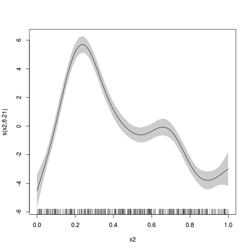
plot (dat.gam, select= 2 , shade= TRUE )
GAM
Interactions
library (mgcv)
dat.gam <- gam (y~s (x2,x3), data= dat)
summary (dat.gam)
GAM
Family: gaussian
Link function: identity

Formula:
y ~ s(x2, x3)

Parametric coefficients:
            Estimate Std. Error t value Pr(>|t|)
(Intercept)    7.728      0.135    57.4   <2e-16

(Intercept) ***
---
Signif. codes:
0 '***' 0.001 '**' 0.01 '*' 0.05 '.' 0.1 ' ' 1

Approximate significance of smooth terms:
          edf Ref.df    F p-value
s(x2,x3) 25.9   28.4 15.9  <2e-16 ***
---
Signif. codes:
0 '***' 0.001 '**' 0.01 '*' 0.05 '.' 0.1 ' ' 1

R-sq.(adj) =  0.528   Deviance explained = 55.8%
GCV = 7.7651  Scale est. = 7.2425    n = 400
GAM
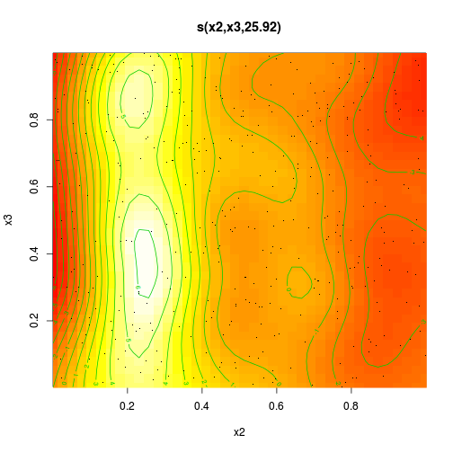
plot (dat.gam, pages= 1 , scheme= 2 )
GAM
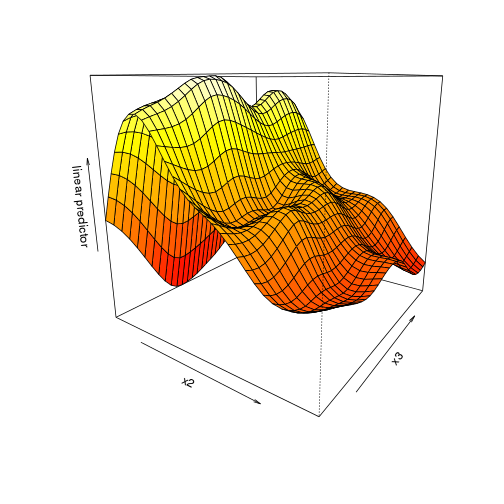
vis.gam (dat.gam, theta= 35 )
GAM
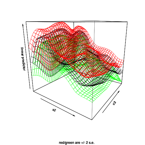
vis.gam (dat.gam, theta= 35 , se= 2 )
GAM Examples 1
data.gp <- read.csv ('../data/data.gp.csv' )
ggplot (data.gp, aes (y= y, x= x))+geom_point ()+geom_line ()+
theme_classic ()
GAM Examples 1
library (mgcv)
data.gp.gam <- gam (y~s (x,k= 3 ), data= data.gp)
summary (data.gp.gam)
Family: gaussian
Link function: identity
Formula:
y ~ s(x, k = 3)
Parametric coefficients:
Estimate Std. Error t value Pr(>|t|)
(Intercept) 9.93e-17 2.87e-01 0 1
Approximate significance of smooth terms:
edf Ref.df F p-value
s(x) 1.95 2 10.9 0.081 .
---
Signif. codes:
0 '***' 0.001 '**' 0.01 '*' 0.05 '.' 0.1 ' ' 1
R-sq.(adj) = 0.835 Deviance explained = 91.5%
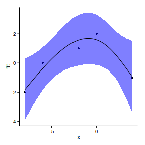
GCV = 1.0045 Scale est. = 0.41203 n = 5plot (data.gp.gam, resid= TRUE , cex= 4 )
Examples 1
xs <- seq (-8 ,4 ,l= 100 )
pred <- predict (data.gp.gam,
newdata = data.frame (x= xs), se= TRUE )
dat <- data.frame (x= xs,fit= pred$fit,
lower= pred$fit-2 *pred$se.fit,
upper= pred$fit+2 *pred$se.fit)
ggplot (data= dat, aes (y= fit, x= x)) +
geom_ribbon (data= dat,
aes (y= fit, x= x, ymin= lower, ymax= upper),
fill= 'blue' ,alpha= 0.2 )+
geom_line ()+
geom_point (data= data.gp, aes (y= y,x= x))+
theme_classic ()
Examples 1
AIC (data.gp.gam)[1] 15.2
GAM Examples 1
library (mgcv)
data.gp.gam <- gam (y~s (x,k= 3 ), data= data.gp)
summary (data.gp.gam)
Family: gaussian
Link function: identity

Formula:
y ~ s(x, k = 3)

Parametric coefficients:
            Estimate Std. Error t value Pr(>|t|)
(Intercept) 9.93e-17   2.87e-01       0        1

Approximate significance of smooth terms:
      edf Ref.df    F p-value
s(x) 1.95      2 10.9   0.081 .
---
Signif. codes:
0 '***' 0.001 '**' 0.01 '*' 0.05 '.' 0.1 ' ' 1

R-sq.(adj) =  0.835   Deviance explained = 91.5%
GCV = 1.0045  Scale est. = 0.41203   n = 5
Examples 1
xs <- seq (-8 ,4 ,l= 100 )
pred <- predict (data.gp.gam,
newdata = data.frame (x= xs), se= TRUE )
dat <- data.frame (x= xs,fit= pred$fit,
lower= pred$fit-2 *pred$se.fit,
upper= pred$fit+2 *pred$se.fit)
head (dat) x fit lower upper
1 -8.000 -1.841 -2.946 -0.7368
2 -7.879 -1.742 -2.815 -0.6687
3 -7.758 -1.643 -2.686 -0.5998
4 -7.636 -1.544 -2.557 -0.5302
5 -7.515 -1.445 -2.430 -0.4597
6 -7.394 -1.346 -2.304 -0.3885ggplot (data= dat, aes (y= fit, x= x)) +
geom_ribbon (data= dat,
aes (y= fit, x= x, ymin= lower, ymax= upper),
fill= 'blue' ,alpha= 0.2 )+
geom_line ()+
geom_point (data= data.gp, aes (y= y,x= x))+
theme_classic ()
Examples 1
AIC (data.gp.gam)[1] 15.2