Linear modelling assumptions

\[ \begin{align*} y_{i} &= \beta_0 + \beta_1 \times x_{i} + \varepsilon_i\\ \epsilon_i&\sim\mathcal{N}(0, \sigma^2) \\ \end{align*} \]

Linear modelling assumptions

\[ \begin{align*} y_{i} &= \beta_0 + \beta_1 \times x_{i} + \varepsilon_i\\ \epsilon_i&\sim\mathcal{N}(0, \sigma^2) \\ \end{align*} \]

Dealing with Heterogeneity

y	x
41.9	1
48.5	2
43	3
51.4	4
51.2	5
37.7	6
50.7	7
65.1	8
51.7	9
38.9	10
70.6	11
51.4	12
62.7	13
34.9	14
95.3	15
63.9	16

Dealing with Heterogeneity

data1 <- read.csv('../data/D1.csv')
summary(data1)

       y              x        
 Min.   :34.9   Min.   : 1.00  
 1st Qu.:42.7   1st Qu.: 4.75  
 Median :51.3   Median : 8.50  
 Mean   :53.7   Mean   : 8.50  
 3rd Qu.:63.0   3rd Qu.:12.25  
 Max.   :95.3   Max.   :16.00

\[ \begin{align*} y_{i} &= \beta_0 + \beta_1 \times x_{i} + \varepsilon_i\\ \epsilon_i&\sim\mathcal{N}(0, \sigma^2) \\ \end{align*} \]

estimate \(\beta_0\), \(\beta_1\) and \(\sigma^2\)

Dealing with Heterogeneity

Dealing with Heterogeneity

Dealing with Heterogeneity

\[ \mathbf{V} = cov = \underbrace{ \begin{pmatrix} \sigma^2&0&0&0&0&0&0&0&0&0&0&0&0&0&0\\ 0&\sigma^2&0&0&0&0&0&0&0&0&0&0&0&0&0\\ 0&0&\sigma^2&0&0&0&0&0&0&0&0&0&0&0&0\\ 0&0&0&\sigma^2&0&0&0&0&0&0&0&0&0&0&0\\ 0&0&0&0&\sigma^2&0&0&0&0&0&0&0&0&0&0\\ 0&0&0&0&0&\sigma^2&0&0&0&0&0&0&0&0&0\\ 0&0&0&0&0&0&\sigma^2&0&0&0&0&0&0&0&0\\ 0&0&0&0&0&0&0&\sigma^2&0&0&0&0&0&0&0\\ 0&0&0&0&0&0&0&0&\sigma^2&0&0&0&0&0&0\\ 0&0&0&0&0&0&0&0&0&\sigma^2&0&0&0&0&0\\ 0&0&0&0&0&0&0&0&0&0&\sigma^2&0&0&0&0\\ 0&0&0&0&0&0&0&0&0&0&0&\sigma^2&0&0&0\\ 0&0&0&0&0&0&0&0&0&0&0&0&\sigma^2&0&0\\ 0&0&0&0&0&0&0&0&0&0&0&0&0&\sigma^2&0\\ 0&0&0&0&0&0&0&0&0&0&0&0&0&0&\sigma^2\\ \end{pmatrix}}_\text{Variance-covariance matrix} \]

Dealing with Heterogeneity

\[ \mathbf{V} = \sigma^2\times \underbrace{ \begin{pmatrix} 1&0&\cdots&0\\ 0&1&\cdots&\vdots\\ \vdots&\cdots&1&\vdots\\ 0&\cdots&\cdots&1\\ \end{pmatrix}}_\text{Identity matrix} = \underbrace{ \begin{pmatrix} \sigma^2&0&\cdots&0\\ 0&\sigma^2&\cdots&\vdots\\ \vdots&\cdots&\sigma^2&\vdots\\ 0&\cdots&\cdots&\sigma^2\\ \end{pmatrix}}_\text{Variance-covariance matrix} \]

Dealing with Heterogeneity

variance proportional to X
variance inversely proportional to X

Dealing with Heterogeneity

variance inversely proportional to X

\[ \mathbf{V} = \sigma^2\times X\times \underbrace{ \begin{pmatrix} 1&0&\cdots&0\\ 0&1&\cdots&\vdots\\ \vdots&\cdots&1&\vdots\\ 0&\cdots&\cdots&1\\ \end{pmatrix}}_\text{Identity matrix} = \underbrace{ \begin{pmatrix} \sigma^2\times \frac{1}{\sqrt{X_1}}&0&\cdots&0\\ 0&\sigma^2\times \frac{1}{\sqrt{X_2}}&\cdots&\vdots\\ \vdots&\cdots&\sigma^2\times \frac{1}{\sqrt{X_i}}&\vdots\\ 0&\cdots&\cdots&\sigma^2\times \frac{1}{\sqrt{X_n}}\\ \end{pmatrix}}_\text{Variance-covariance matrix} \]

Dealing with Heterogeneity

\[ \mathbf{V} = \sigma^2\times \omega, \hspace{1cm} \text{where } \omega = \underbrace{ \begin{pmatrix} \frac{1}{\sqrt{X_1}}&0&\cdots&0\\ 0&\frac{1}{\sqrt{X_2}}&\cdots&\vdots\\ \vdots&\cdots&\frac{1}{\sqrt{X_i}}&\vdots\\ 0&\cdots&\cdots&\frac{1}{\sqrt{X_n}}\\ \end{pmatrix}}_\text{Weights matrix} \]

Dealing with Heterogeneity

Calculating weights

1/sqrt(data1$x)

 [1] 1.0000 0.7071 0.5774 0.5000 0.4472 0.4082
 [7] 0.3780 0.3536 0.3333 0.3162 0.3015 0.2887
[13] 0.2774 0.2673 0.2582 0.2500

Generalized least squares (GLS)

use OLS to estimate fixed effects
use these estimates to estimate variances via ML
use these to re-estimate fixed effects (OLS)

Generalized least squares (GLS)

ML is biased (for variance) when N is small:

use REML
max. likelihood of residuals rather than data

Variance structures

Variance function	Variance structure	Description
`varFixed(~x)`	\(V = \sigma^2\times x\)	variance proportional to `x` the covariate
`varExp(form=~x)`	\(V = \sigma^2\times e^{2\delta\times x}\)	variance proportional to the exponential of `x` multiplied by a constant
`varPower(form=~x)`	\(V = \sigma^2\times \|x\|^{2\delta}\)	variance proportional to the absolute value of `x` raised to a constant power
`varConstPower(form=~x)`	\(V = \sigma^2\times (\delta_1 + \|x\|^{\delta_2})^2\)	a variant on the power function
`varIdent(form=~\|A)`	\(V = \sigma_j^2\times I\)	when `A` is a factor, variance is allowed to be different for each level (\(j\)) of the factor
`varComb(form=~x\|A)`	\(V = \sigma_j^2\times x\)	combination of two of the above

Generalized least squares (GLS)

library(nlme)
data1.gls <- gls(y~x, data1,
                 method='REML')
plot(data1.gls)

library(nlme)
data1.gls1 <- gls(y~x, data=data1, weights=varFixed(~x),
                  method='REML')
plot(data1.gls1)

Generalized least squares (GLS)

wrong

plot(resid(data1.gls) ~
     fitted(data1.gls))

plot(resid(data1.gls1) ~
     fitted(data1.gls1))

Generalized least squares (GLS)

CORRECT

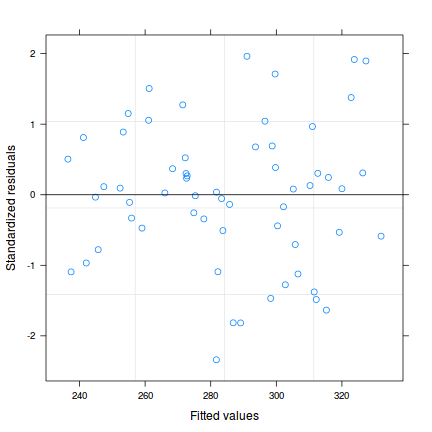
plot(resid(data1.gls,'normalized') ~
     fitted(data1.gls))

plot(resid(data1.gls1,'normalized') ~
     fitted(data1.gls1))

Generalized least squares (GLS)

plot(resid(data1.gls,'normalized') ~ data1$x)

plot(resid(data1.gls1,'normalized') ~ data1$x)

Generalized least squares (GLS)

AIC(data1.gls, data1.gls1)

           df   AIC
data1.gls   3 127.6
data1.gls1  3 121.1

#OR
anova(data1.gls, data1.gls1)

           Model df   AIC   BIC logLik
data1.gls      1  3 127.6 129.6 -60.82
data1.gls1     2  3 121.1 123.0 -57.54

Generalized least squares (GLS)

Can we go better

library(nlme)
data1.gls1 <- gls(y~x, data=data1,
  weights=varFixed(~x),method='REML')
plot(data1.gls1)

library(nlme)
data1.gls2 <- gls(y~x, data=data1,
  weights=varFixed(~x^2),method='REML')
plot(data1.gls2)

Generalized least squares (GLS)

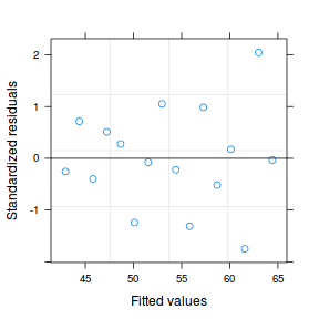
CORRECT

plot(resid(data1.gls1,'normalized') ~
     fitted(data1.gls1))

plot(resid(data1.gls2,'normalized') ~
     fitted(data1.gls2))

Generalized least squares (GLS)

AIC(data1.gls, data1.gls1, data1.gls2)

           df   AIC
data1.gls   3 127.6
data1.gls1  3 121.1
data1.gls2  3 119.0

#OR
anova(data1.gls, data1.gls1, data1.gls2)

           Model df   AIC   BIC logLik
data1.gls      1  3 127.6 129.6 -60.82
data1.gls1     2  3 121.1 123.0 -57.54
data1.gls2     3  3 119.0 120.9 -56.50

Generalized least squares (GLS)

summary(data1.gls)

Generalized least squares fit by REML
  Model: y ~ x 
  Data: data1 
    AIC   BIC logLik
  127.6 129.6 -60.82

Coefficients:
            Value Std.Error t-value p-value
(Intercept) 40.33     7.189   5.610  0.0001
x            1.57     0.744   2.113  0.0531

 Correlation: 
  (Intr)
x -0.879

Standardized residuals:
     Min       Q1      Med       Q3      Max 
-2.00006 -0.29320 -0.02283  0.35358  2.29100 

Residual standard error: 13.71 
Degrees of freedom: 16 total; 14 residual

summary(data1.gls2)

Generalized least squares fit by REML
  Model: y ~ x 
  Data: data1 
  AIC   BIC logLik
  119 120.9  -56.5

Variance function:
 Structure: fixed weights
 Formula: ~x^2 

Coefficients:
            Value Std.Error t-value p-value
(Intercept) 41.22     1.494  27.598  0.0000
x            1.49     0.470   3.176  0.0067

 Correlation: 
  (Intr)
x -0.671

Standardized residuals:
     Min       Q1      Med       Q3      Max 
-1.49260 -0.59853 -0.07669  0.77799  1.54158 

Residual standard error: 1.393 
Degrees of freedom: 16 total; 14 residual

Generalized least squares (GLS)

data1$cx <- scale(data1$x, scale=FALSE)
data1.gls <- gls(y~cx, data1,
                 method='REML')
summary(data1.gls)

Generalized least squares fit by REML
  Model: y ~ cx 
  Data: data1 
    AIC   BIC logLik
  127.6 129.6 -60.82

Coefficients:
            Value Std.Error t-value p-value
(Intercept) 53.68     3.427  15.662  0.0000
cx           1.57     0.744   2.113  0.0531

 Correlation: 
   (Intr)
cx 0     

Standardized residuals:
     Min       Q1      Med       Q3      Max 
-2.00006 -0.29320 -0.02283  0.35358  2.29100 

Residual standard error: 13.71 
Degrees of freedom: 16 total; 14 residual

data1$cx <- scale(data1$x, scale=FALSE)
data1.gls2 <- gls(y~cx, data1,
                  weights=varFixed(~x^2), method='REML')
summary(data1.gls2)

Generalized least squares fit by REML
  Model: y ~ cx 
  Data: data1 
  AIC   BIC logLik
  119 120.9  -56.5

Variance function:
 Structure: fixed weights
 Formula: ~x^2 

Coefficients:
            Value Std.Error t-value p-value
(Intercept) 53.91      3.19  16.898  0.0000
cx           1.49      0.47   3.176  0.0067

 Correlation: 
   (Intr)
cx 0.938 

Standardized residuals:
     Min       Q1      Med       Q3      Max 
-1.49260 -0.59853 -0.07669  0.77799  1.54158 

Residual standard error: 1.393 
Degrees of freedom: 16 total; 14 residual

Heteroscadacity in ANOVA

data2 <- read.csv('../data/D2.csv')
summary(data2)

       y        x     
 Min.   :29.3   A:10  
 1st Qu.:36.2   B:10  
 Median :40.9   C:10  
 Mean   :42.3   D:10  
 3rd Qu.:49.3   E:10  
 Max.   :56.8

\[ \begin{align*} y_{i} &= \mu + \alpha_i + \varepsilon_i\\ \epsilon_i&\sim\mathcal{N}(0, \sigma^2) \\ \end{align*} \]

estimate \(\mu\), \(\alpha_i\) and \(\sigma^2\)

Heteroscadacity in ANOVA

boxplot(y~x, data2)

Heteroscadacity in ANOVA

plot(lm(y~x, data2), which=3)

Heteroscadacity in ANOVA

\[\varepsilon \sim \mathcal{N}(0,\sigma_i^2\times \omega)\]

\[\text{Effect (}\alpha\text{) 1 (i=1)} \quad \begin{pmatrix} y_{1i}\\ y_{2i}\\ y_{3i}\\ \end{pmatrix} = \begin{pmatrix} 1&1&0&0\\ 1&1&0&0\\ 1&1&0&0\\ \end{pmatrix} \times \begin{pmatrix} \beta_i \end{pmatrix} + \begin{pmatrix} \varepsilon_{1i}\\ \varepsilon_{2i}\\ \varepsilon_{3i} \end{pmatrix} \quad \varepsilon_i \sim \mathcal{N}(0, \begin{pmatrix} \sigma_1^2&0&0\\ 0&\sigma_1^2&0\\ 0&0&\sigma_1^2 \end{pmatrix} ) \] \[\text{Effect (}\alpha\text{) 2 (i=2)} \quad \begin{pmatrix} y_{1i}\\ y_{2i}\\ y_{3i}\\ \end{pmatrix} = \begin{pmatrix} 1&0&1&0\\ 1&0&1&0\\ 1&0&1&0\\ \end{pmatrix} \times \begin{pmatrix} \beta_i \end{pmatrix} + \begin{pmatrix} \varepsilon_{1i}\\ \varepsilon_{2i}\\ \varepsilon_{3i} \end{pmatrix} \quad \varepsilon_i \sim \mathcal{N}(0, \begin{pmatrix} \sigma_2^2&0&0\\ 0&\sigma_2^2&0\\ 0&0&\sigma_2^2 \end{pmatrix} ) \] \[\text{Effect (}\alpha\text{) 3 (i=3)} \quad \begin{pmatrix} y_{1i}\\ y_{2i}\\ y_{3i}\\ \end{pmatrix} = \begin{pmatrix} 1&0&0&1\\ 1&0&0&1\\ 1&0&0&1\\ \end{pmatrix} \times \begin{pmatrix} \beta_i \end{pmatrix} + \begin{pmatrix} \varepsilon_{1i}\\ \varepsilon_{2i}\\ \varepsilon_{3i} \end{pmatrix} \quad \varepsilon_i \sim \mathcal{N}(0, \begin{pmatrix} \sigma_3^2&0&0\\ 0&\sigma_3^2&0\\ 0&0&\sigma_3^2 \end{pmatrix} ) \]

Heteroscadacity in ANOVA

\[ V_{ji} = \begin{pmatrix} \sigma_1^2&0&0&0&0&0&0&0&0\\ 0&\sigma_1^2&0&0&0&0&0&0&0\\ 0&0&\sigma_1^2&0&0&0&0&0&0\\ 0&0&0&\sigma_2^2&0&0&0&0&0\\ 0&0&0&0&\sigma_2^2&0&0&0&0\\ 0&0&0&0&0&\sigma_2^2&0&0&0\\ 0&0&0&0&0&0&\sigma_3^2&0&0\\ 0&0&0&0&0&0&0&\sigma_3^2&0\\ 0&0&0&0&0&0&0&0&\sigma_3^2\\ \end{pmatrix} \]

Heteroscadacity in ANOVA

data2.sd <- with(data2, tapply(y,x,sd))
1/(data2.sd[1]/data2.sd)

      A       B       C       D       E 
1.00000 0.91343 0.40807 0.08632 0.12720

Variance structures

Variance function	Variance structure	Description
`varFixed(~x)`	\(V = \sigma^2\times x\)	variance proportional to `x` the covariate
`varExp(form=~x)`	\(V = \sigma^2\times e^{2\delta\times x}\)	variance proportional to the exponential of `x` multiplied by a constant
`varPower(form=~x)`	\(V = \sigma^2\times \|x\|^{2\delta}\)	variance proportional to the absolute value of `x` raised to a constant power
`varConstPower(form=~x)`	\(V = \sigma^2\times (\delta_1 + \|x\|^{\delta_2})^2\)	a variant on the power function
`varIdent(form=~\|A)`	\(V = \sigma_j^2\times I\)	when `A` is a factor, variance is allowed to be different for each level (\(j\)) of the factor
`varComb(form=~x\|A)`	\(V = \sigma_j^2\times x\)	combination of two of the above

Heteroscadacity in ANOVA

library(nlme)
data2.gls <- gls(y~x, data=data2,
                 method="REML")

library(nlme)
data2.gls1 <- gls(y~x, data=data2,
   weights=varIdent(form=~1|x), method="REML")

Heteroscadacity in ANOVA

library(nlme)
data2.gls <- gls(y~x, data=data2,
                 method="REML")
plot(resid(data2.gls,'normalized') ~
     fitted(data2.gls))

library(nlme)
data2.gls1 <- gls(y~x, data=data2,
   weights=varIdent(form=~1|x), method="REML")
plot(resid(data2.gls1,'normalized') ~
     fitted(data2.gls1))

Heteroscadacity in ANOVA

AIC(data2.gls,data2.gls1)

           df   AIC
data2.gls   6 249.5
data2.gls1 10 199.2

anova(data2.gls,data2.gls1)

           Model df   AIC   BIC logLik   Test
data2.gls      1  6 249.5 260.3 -118.8       
data2.gls1     2 10 199.2 217.3  -89.6 1 vs 2
           L.Ratio p-value
data2.gls                 
data2.gls1   58.29  <.0001

note: it costs d.f.

Heteroscadacity in ANOVA

summary(data2.gls)

Generalized least squares fit by REML
  Model: y ~ x 
  Data: data2 
    AIC   BIC logLik
  249.5 260.3 -118.7

Coefficients:
             Value Std.Error t-value p-value
(Intercept)  40.79    0.9424   43.29  0.0000
xB            5.20    1.3328    3.90  0.0003
xC           13.94    1.3328   10.46  0.0000
xD           -0.73    1.3328   -0.55  0.5851
xE          -10.66    1.3328   -8.00  0.0000

 Correlation: 
   (Intr) xB     xC     xD    
xB -0.707                     
xC -0.707  0.500              
xD -0.707  0.500  0.500       
xE -0.707  0.500  0.500  0.500

Standardized residuals:
     Min       Q1      Med       Q3      Max 
-3.30654 -0.24626  0.06468  0.39047  2.94559 

Residual standard error: 2.98 
Degrees of freedom: 50 total; 45 residual

summary(data2.gls1)

Generalized least squares fit by REML
  Model: y ~ x 
  Data: data2 
    AIC   BIC logLik
  199.2 217.3  -89.6

Variance function:
 Structure: Different standard deviations per stratum
 Formula: ~1 | x 
 Parameter estimates:
      A       B       C       D       E 
1.00000 0.91342 0.40807 0.08632 0.12720 

Coefficients:
             Value Std.Error t-value p-value
(Intercept)  40.79     1.481  27.543  0.0000
xB            5.20     2.006   2.593  0.0128
xC           13.94     1.600   8.714  0.0000
xD           -0.73     1.487  -0.493  0.6244
xE          -10.66     1.493  -7.139  0.0000

 Correlation: 
   (Intr) xB     xC     xD    
xB -0.738                     
xC -0.926  0.684              
xD -0.996  0.736  0.922       
xE -0.992  0.732  0.918  0.988

Standardized residuals:
    Min      Q1     Med      Q3     Max 
-2.3034 -0.6179  0.1065  0.7597  1.8743 

Residual standard error: 4.684 
Degrees of freedom: 50 total; 45 residual

Bayesian

library(R2jags)

modelString = "
model {
   #Likelihood
   for (i in 1:n) {
      y[i]~dnorm(mu[i],tau)
      mu[i] <- beta0+beta1*x[i]
   }
 
   #Priors
   beta0 ~ dnorm(0.01,1.0E-6)
   beta1 ~ dnorm(0,1.0E-6)
   tau <- 1 / (sigma*sigma)     
   sigma~dunif(0,100)
 }
"

writeLines(modelString, con='../BUGSscripts/simpleRegression.JAGS')

data1.list <- list(y = data1$y, x = data1$x,
      n = nrow(data1))

params <- c("beta0", "beta1", "sigma")
nChains = 3
burnInSteps = 3000
thinSteps = 10
numSavedSteps = 15000 
nIter = ceiling(burnInSteps+(numSavedSteps * thinSteps)/nChains)
nIter

[1] 53000

data1.r2jags <- jags(data=data1.list, 
           inits=NULL, 
           parameters.to.save=params,
           model.file="../BUGSscripts/simpleRegression.JAGS",
           n.chains=nChains,
           n.iter=nIter,
           n.burnin=burnInSteps,
           n.thin=thinSteps
           )

Compiling model graph
   Resolving undeclared variables
   Allocating nodes
   Graph Size: 121

Initializing model

print(data1.r2jags)

Inference for Bugs model at "../BUGSscripts/simpleRegression.JAGS", fit using jags,
 3 chains, each with 53000 iterations (first 3000 discarded), n.thin = 10
 n.sims = 15000 iterations saved
         mu.vect sd.vect    2.5%     25%     50%
beta0     50.503   2.642  45.318  48.742  50.509
beta1     -2.716   0.799  -4.283  -3.259  -2.707
sigma      7.965   0.844   6.540   7.377   7.889
deviance 347.934   2.585 345.008 346.051 347.273
             75%   97.5%  Rhat n.eff
beta0     52.251  55.705 1.001 15000
beta1     -2.185  -1.154 1.001 15000
sigma      8.487   9.856 1.001 15000
deviance 349.079 354.550 1.001  3700

For each parameter, n.eff is a crude measure of effective sample size,
and Rhat is the potential scale reduction factor (at convergence, Rhat=1).

DIC info (using the rule, pD = var(deviance)/2)
pD = 3.3 and DIC = 351.3
DIC is an estimate of expected predictive error (lower deviance is better).

summary(data1.gls)

Generalized least squares fit by REML
  Model: y ~ cx 
  Data: data1 
    AIC   BIC logLik
  127.6 129.6 -60.82

Coefficients:
            Value Std.Error t-value p-value
(Intercept) 53.68     3.427  15.662  0.0000
cx           1.57     0.744   2.113  0.0531

 Correlation: 
   (Intr)
cx 0     

Standardized residuals:
     Min       Q1      Med       Q3      Max 
-2.00006 -0.29320 -0.02283  0.35358  2.29100 

Residual standard error: 13.71 
Degrees of freedom: 16 total; 14 residual

data1.gls$sigma

[1] 13.71

modelString = "
model {
   #Likelihood
   for (i in 1:n) {
      y[i]~dnorm(mu[i],tau*(1/x[i]))
      mu[i] <- beta0+beta1*x[i]
   }
 
   #Priors
   beta0 ~ dnorm(0.01,1.0E-6)
   beta1 ~ dnorm(0,1.0E-6)
   tau <- 1 / (sigma*sigma)     
   sigma~dunif(0,100)
 }
"

writeLines(modelString, con='../BUGSscripts/simpleRegression1.JAGS')

data1.list <- with(data1, list(y = y, x = x, n = nrow(data1)))

params <- c("beta0", "beta1", "sigma")
nChains = 3
burnInSteps = 3000
thinSteps = 10
numSavedSteps = 15000 
nIter = ceiling(burnInSteps+(numSavedSteps * thinSteps)/nChains)
nIter

[1] 53000

data1.r2jags1 <- jags(data=data1.list, 
           inits=NULL, 
           parameters.to.save=params,
           model.file="../BUGSscripts/simpleRegression1.JAGS",
           n.chains=nChains,
           n.iter=nIter,
           n.burnin=burnInSteps,
           n.thin=thinSteps
           )

Compiling model graph
   Resolving undeclared variables
   Allocating nodes
   Graph Size: 131

Initializing model

print(data1.r2jags1)

Inference for Bugs model at "../BUGSscripts/simpleRegression1.JAGS", fit using jags,
 3 chains, each with 53000 iterations (first 3000 discarded), n.thin = 10
 n.sims = 15000 iterations saved
         mu.vect sd.vect    2.5%     25%     50%
beta0     44.620   2.047  40.624  43.260  44.609
beta1     -0.756   0.797  -2.317  -1.288  -0.756
sigma      5.080   0.535   4.156   4.703   5.032
deviance 350.703   2.555 347.786 348.829 350.061
             75%   97.5%  Rhat n.eff
beta0     46.001  48.639 1.001 15000
beta1     -0.222   0.803 1.001 15000
sigma      5.407   6.253 1.001 12000
deviance 351.875 357.345 1.001 15000

For each parameter, n.eff is a crude measure of effective sample size,
and Rhat is the potential scale reduction factor (at convergence, Rhat=1).

DIC info (using the rule, pD = var(deviance)/2)
pD = 3.3 and DIC = 354.0
DIC is an estimate of expected predictive error (lower deviance is better).

summary(data1.gls1)

Generalized least squares fit by REML
  Model: y ~ x 
  Data: data1 
    AIC BIC logLik
  121.1 123 -57.54

Variance function:
 Structure: fixed weights
 Formula: ~x 

Coefficients:
            Value Std.Error t-value p-value
(Intercept) 41.50     3.332  12.455  0.0000
x            1.43     0.525   2.727  0.0164

 Correlation: 
  (Intr)
x -0.746

Standardized residuals:
     Min       Q1      Med       Q3      Max 
-1.74684 -0.42653 -0.05467  0.56196  2.04503 

Residual standard error: 4.079 
Degrees of freedom: 16 total; 14 residual

data1.gls1$sigma

[1] 4.079

modelString = "
model {
   #Likelihood
   for (i in 1:n) {
      y[i]~dnorm(mu[i],tau*(1/x[i]^2))
      mu[i] <- beta0+beta1*x[i]
   }
 
   #Priors
   beta0 ~ dnorm(0.01,1.0E-6)
   beta1 ~ dnorm(0,1.0E-6)
   tau <- 1 / (sigma*sigma)     
   sigma~dunif(0,100)
 }
"

writeLines(modelString, con='../BUGSscripts/simpleRegression2.JAGS')

data1.list <- with(data1, list(y = y, x = x, n = nrow(data1)))

params <- c("beta0", "beta1", "sigma")
nChains = 3
burnInSteps = 3000
thinSteps = 10
numSavedSteps = 15000 
nIter = ceiling(burnInSteps+(numSavedSteps * thinSteps)/nChains)
nIter

[1] 53000

data1.r2jags2 <- jags(data=data1.list, 
           inits=NULL, 
           parameters.to.save=params,
           model.file="../BUGSscripts/simpleRegression2.JAGS",
           n.chains=nChains,
           n.iter=nIter,
           n.burnin=burnInSteps,
           n.thin=thinSteps
           )

Compiling model graph
   Resolving undeclared variables
   Allocating nodes
   Graph Size: 137

Initializing model

print(data1.r2jags2)

Inference for Bugs model at "../BUGSscripts/simpleRegression2.JAGS", fit using jags,
 3 chains, each with 53000 iterations (first 3000 discarded), n.thin = 10
 n.sims = 15000 iterations saved
         mu.vect sd.vect    2.5%     25%     50%
beta0     41.087   1.666  37.792  39.985  41.076
beta1      0.846   0.900  -0.915   0.251   0.844
sigma      3.390   0.357   2.772   3.135   3.363
deviance 358.160   2.585 355.239 356.287 357.494
             75%   97.5%  Rhat n.eff
beta0     42.195  44.356 1.001 14000
beta1      1.442   2.618 1.001 15000
sigma      3.612   4.174 1.001 15000
deviance 359.321 364.845 1.001 15000

For each parameter, n.eff is a crude measure of effective sample size,
and Rhat is the potential scale reduction factor (at convergence, Rhat=1).

DIC info (using the rule, pD = var(deviance)/2)
pD = 3.3 and DIC = 361.5
DIC is an estimate of expected predictive error (lower deviance is better).

summary(data1.gls2)

Generalized least squares fit by REML
  Model: y ~ cx 
  Data: data1 
  AIC   BIC logLik
  119 120.9  -56.5

Variance function:
 Structure: fixed weights
 Formula: ~x^2 

Coefficients:
            Value Std.Error t-value p-value
(Intercept) 53.91      3.19  16.898  0.0000
cx           1.49      0.47   3.176  0.0067

 Correlation: 
   (Intr)
cx 0.938 

Standardized residuals:
     Min       Q1      Med       Q3      Max 
-1.49260 -0.59853 -0.07669  0.77799  1.54158 

Residual standard error: 1.393 
Degrees of freedom: 16 total; 14 residual

data1.gls2$sigma

[1] 1.393

modelString="
model {
   #Likelihood
   for (i in 1:n) {
      y[i]~dnorm(mean[i],tau)
      mean[i] <- X[i,] %*% beta
   }

   #Priors and derivatives
   for (i in 1:ngroups) {
     beta[i] ~ dnorm(0, 1.0E-6)
   }
   sigma ~ dunif(0, 1000)
   tau <- 1 / (sigma * sigma)
}
"
writeLines(modelString,con="../BUGSscripts/simpleANOVA.JAGS")
X <- model.matrix(~x, data2)
data2.list <- list(y=data2$y, X=X, n=nrow(data2), ngroups=ncol(X))

params <- c("beta","sigma")
burnInSteps = 2000
nChains = 3 
numSavedSteps = 50000
thinSteps = 10
nIter = ceiling((numSavedSteps * thinSteps)/nChains)

library(R2jags)
data2.r2jags <- jags(data=data2.list, 
      inits=NULL,
      parameters.to.save=params, 
      model.file="../BUGSscripts/simpleANOVA.JAGS",
      n.chains=3,
      n.iter=nIter, 
      n.burnin=burnInSteps,
      n.thin=thinSteps
      )

Compiling model graph
   Resolving undeclared variables
   Allocating nodes
   Graph Size: 370

Initializing model

print(data2.r2jags)

Inference for Bugs model at "../BUGSscripts/simpleANOVA.JAGS", fit using jags,
 3 chains, each with 166667 iterations (first 2000 discarded), n.thin = 10
 n.sims = 49401 iterations saved
         mu.vect sd.vect    2.5%     25%     50%
beta[1]   40.800   0.976  38.869  40.154  40.806
beta[2]    5.188   1.379   2.495   4.265   5.184
beta[3]   13.930   1.380  11.229  13.018  13.927
beta[4]   -0.744   1.379  -3.433  -1.661  -0.746
beta[5]  -10.662   1.378 -13.367 -11.581 -10.664
sigma      3.068   0.334   2.498   2.832   3.039
deviance 252.356   3.766 247.195 249.599 251.639
             75%   97.5%  Rhat n.eff
beta[1]   41.451  42.707 1.001 49000
beta[2]    6.099   7.906 1.001 49000
beta[3]   14.843  16.655 1.001 49000
beta[4]    0.171   1.986 1.001 49000
beta[5]   -9.751  -7.946 1.001 49000
sigma      3.271   3.803 1.001 40000
deviance 254.374 261.631 1.001 49000

For each parameter, n.eff is a crude measure of effective sample size,
and Rhat is the potential scale reduction factor (at convergence, Rhat=1).

DIC info (using the rule, pD = var(deviance)/2)
pD = 7.1 and DIC = 259.4
DIC is an estimate of expected predictive error (lower deviance is better).

summary(data2.gls)

Generalized least squares fit by REML
  Model: y ~ x 
  Data: data2 
    AIC   BIC logLik
  249.5 260.3 -118.7

Coefficients:
             Value Std.Error t-value p-value
(Intercept)  40.79    0.9424   43.29  0.0000
xB            5.20    1.3328    3.90  0.0003
xC           13.94    1.3328   10.46  0.0000
xD           -0.73    1.3328   -0.55  0.5851
xE          -10.66    1.3328   -8.00  0.0000

 Correlation: 
   (Intr) xB     xC     xD    
xB -0.707                     
xC -0.707  0.500              
xD -0.707  0.500  0.500       
xE -0.707  0.500  0.500  0.500

Standardized residuals:
     Min       Q1      Med       Q3      Max 
-3.30654 -0.24626  0.06468  0.39047  2.94559 

Residual standard error: 2.98 
Degrees of freedom: 50 total; 45 residual

data2$sigma

NULL

modelString="
model {
   #Likelihood
   for (i in 1:n) {
      y[i]~dnorm(mean[i],tau[x[i]])
      mean[i] <- X[i,] %*% eta
   }

   #Priors and derivatives
   for (i in 1:ngroups) {
     beta[i] ~ dnorm(0, 1.0E-6) #prior
     sigma[i] ~ dgamma(0.001, 0.001)
     tau[i] <- 1 / (sigma[i] * sigma[i])
   }
}
"
writeLines(modelString,con="../BUGSscripts/simpleANOVA1.JAGS")
X <- model.matrix(~x, data2)
data2.list <- list(y=data2$y, X=X, x=as.numeric(data2$x), n=nrow(data2), ngroups=ncol(X))

params <- c("beta","sigma")
burnInSteps = 2000
nChains = 3 
numSavedSteps = 50000
thinSteps = 10
nIter = ceiling((numSavedSteps * thinSteps)/nChains)

library(R2jags)
data2.r2jags1 <- jags(data=data2.list, 
      inits=NULL,
      parameters.to.save=params, 
      model.file="../BUGSscripts/simpleANOVA1.JAGS",
      n.chains=3,
      n.iter=nIter, 
      n.burnin=burnInSteps,
      n.thin=thinSteps
      )

Compiling model graph
   Resolving undeclared variables
   Allocating nodes
Deleting model

Error: RUNTIME ERROR:
Compilation error on line 5.
Unable to resolve node mean[1]
This may be due to an undefined ancestor node or a directed cycle in the graph

print(data2.r2jags1)

Error: object 'data2.r2jags1' not found

summary(data2.gls1)

Generalized least squares fit by REML
  Model: y ~ x 
  Data: data2 
    AIC   BIC logLik
  199.2 217.3  -89.6

Variance function:
 Structure: Different standard deviations per stratum
 Formula: ~1 | x 
 Parameter estimates:
      A       B       C       D       E 
1.00000 0.91342 0.40807 0.08632 0.12720 

Coefficients:
             Value Std.Error t-value p-value
(Intercept)  40.79     1.481  27.543  0.0000
xB            5.20     2.006   2.593  0.0128
xC           13.94     1.600   8.714  0.0000
xD           -0.73     1.487  -0.493  0.6244
xE          -10.66     1.493  -7.139  0.0000

 Correlation: 
   (Intr) xB     xC     xD    
xB -0.738                     
xC -0.926  0.684              
xD -0.996  0.736  0.922       
xE -0.992  0.732  0.918  0.988

Standardized residuals:
    Min      Q1     Med      Q3     Max 
-2.3034 -0.6179  0.1065  0.7597  1.8743 

Residual standard error: 4.684 
Degrees of freedom: 50 total; 45 residual

data2.gls1$sigma

[1] 4.684

Linear modelling assumptions

\[ \begin{align*} y_{i} &= \beta_0 + \beta_1 \times x_{i} + \varepsilon_i\\ \epsilon_i&\sim\mathcal{N}(0, \sigma^2) \\ \end{align*} \]

Non-independence

one response is triggered by another
temporal/spatial autocorrelation
nested (hierarchical) design structures

Variance-covariance

\[ \mathbf{V} = \underbrace{ \begin{pmatrix} \sigma^2&0&\cdots&0\\ 0&\sigma^2&\cdots&\vdots\\ \vdots&\cdots&\sigma^2&\vdots\\ 0&\cdots&\cdots&\sigma^2\\ \end{pmatrix}}_\text{Variance-covariance matrix} \]

Compound symmetry

constant correlation (and cov)
sphericity

\[ cor(\varepsilon)= \underbrace{ \begin{pmatrix} 1&\rho&\cdots&\rho\\ \rho&1&\cdots&\vdots\\ \dots&\cdots&1&\vdots\\ \rho&\cdots&\cdots&1\\ \end{pmatrix}}_\text{Correlation matrix} \] \[ \mathbf{V} = \underbrace{ \begin{pmatrix} \theta + \sigma^2&\theta&\cdots&\theta\\ \theta&\theta + \sigma^2&\cdots&\vdots\\ \vdots&\cdots&\theta + \sigma^2&\vdots\\ \theta&\cdots&\cdots&\theta + \sigma^2\\ \end{pmatrix}}_\text{Variance-covariance matrix} \]

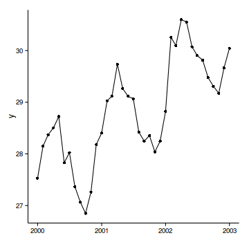
Temporal autocorrelation

correlation dependent on proximity
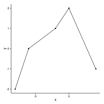
data.t

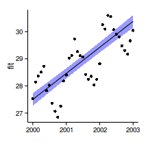
Temporal autocorrelation

Relationship between Y and X

data.t.lm <- lm(y~x, data=data.t)
par(mfrow=c(2,3))
plot(data.t.lm, which=1:6, ask=FALSE)

Temporal autocorrelation

Relationship between Y and X

acf(rstandard(data.t.lm))

Temporal autocorrelation

can we partial out time

plot(rstandard(data.t.lm)~data.t$year)

Temporal autocorrelation

can we partial out time

library(car)
vif(lm(y~x+year, data=data.t))

   x year 
1.04 1.04

data.t.lm1 <- lm(y~x+year, data.t)

Testing for autocorrelation

Residual plot

par(mfrow=c(1,2))
plot(rstandard(data.t.lm1)~fitted(data.t.lm1))
plot(rstandard(data.t.lm1)~data.t$year)

Testing for autocorrelation

Autocorrelation (acf) plot

acf(rstandard(data.t.lm1), lag=40)

First order autocorrelation (AR1)

\[ cor(\varepsilon) = \underbrace{ \begin{pmatrix} 1&\rho&\cdots&\rho^{|t-s|}\\ \rho&1&\cdots&\vdots\\ \vdots&\cdots&1&\vdots\\ \rho^{|t-s|}&\cdots&\cdots&1\\ \end{pmatrix}}_\text{First order autoregressive correlation structure} \]

where:

\(s\) and \(t\) are the times.
\(s-t\) is the lag

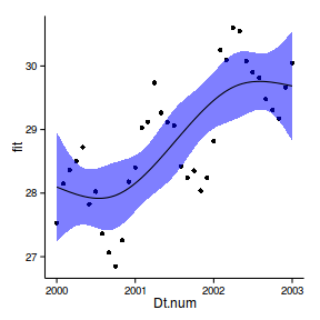
First order auto-regressive (AR1)

library(nlme)
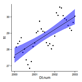
data.t.gls <- gls(y~x+year, data=data.t, method='REML')
data.t.gls1 <- gls(y~x+year, data=data.t,
        correlation=corAR1(form=~year),method='REML')

First order auto-regressive (AR1)

par(mfrow=c(1,2))
plot(residuals(data.t.gls, type="normalized")~
     fitted(data.t.gls))
plot(residuals(data.t.gls1, type="normalized")~
     fitted(data.t.gls1))

First order auto-regressive (AR1)

par(mfrow=c(1,2))
plot(residuals(data.t.gls, type="normalized")~
     data.t$x)
plot(residuals(data.t.gls1, type="normalized")~
     data.t$x)

First order auto-regressive (AR1)

par(mfrow=c(1,2))
plot(residuals(data.t.gls, type="normalized")~
     data.t$year)
plot(residuals(data.t.gls1, type="normalized")~
     data.t$year)

First order auto-regressive (AR1)

par(mfrow=c(1,2))
acf(residuals(data.t.gls, type='normalized'), lag=40)
acf(residuals(data.t.gls1, type='normalized'), lag=40)

First order auto-regressive (AR1)

AIC(data.t.gls, data.t.gls1)

            df   AIC
data.t.gls   4 626.3
data.t.gls1  5 536.7

anova(data.t.gls, data.t.gls1)

            Model df   AIC   BIC logLik   Test
data.t.gls      1  4 626.3 636.6 -309.2       
data.t.gls1     2  5 536.7 549.6 -263.4 1 vs 2
            L.Ratio p-value
data.t.gls                 
data.t.gls1   91.58  <.0001

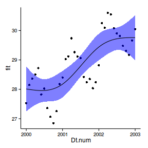
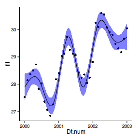
Auto-regressive moving average (ARMA)

data.t.gls2 <- update(data.t.gls,
   correlation=corARMA(form=~year,p=2,q=0))
data.t.gls3 <- update(data.t.gls,
   correlation=corARMA(form=~year,p=3,q=0))
AIC(data.t.gls, data.t.gls1, data.t.gls2, data.t.gls3)

            df   AIC
data.t.gls   4 626.3
data.t.gls1  5 536.7
data.t.gls2  6 538.1
data.t.gls3  7 538.8

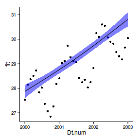
Summarize model

summary(data.t.gls1)

Generalized least squares fit by REML
  Model: y ~ x + year 
  Data: data.t 
    AIC   BIC logLik
  536.7 549.6 -263.4

Correlation Structure: ARMA(1,0)
 Formula: ~year 
 Parameter estimate(s):
  Phi1 
0.9127 

Coefficients:
            Value Std.Error t-value p-value
(Intercept)  4389    1232.6   3.560  0.0006
x               0       0.0   3.297  0.0014
year           -2       0.6  -3.546  0.0006

 Correlation: 
     (Intr) x     
x     0.009       
year -1.000 -0.010

Standardized residuals:
   Min     Q1    Med     Q3    Max 
-1.423  1.711  3.378  4.373  6.624 

Residual standard error: 3.375 
Degrees of freedom: 100 total; 97 residual

Spatial autocorrelation

similar, yet dependency is 2d
2d Euclidean dissimilarity
Exponential decay

\[ cor(\varepsilon) = \underbrace{ \begin{pmatrix} 1&e^{-\delta}&\cdots&e^{-\delta D}\\ e^{-\delta}&1&\cdots&\vdots\\ \vdots&\cdots&1&\vdots\\ e^{-\delta D}&\cdots&\cdots&1\\ \end{pmatrix}}_\text{Exponential autoregressive correlation structure} \]

Spatial autocorrelation

data.s

Spatial autocorrelation

Spatial arrangement of Y

library(sp)
coordinates(data.s) <- ~LAT+LONG
bubble(data.s,'y')

Spatial autocorrelation

Relationship between Y and X

data.s.lm <- lm(y~x, data=data.s)
par(mfrow=c(2,3))
plot(data.s.lm, which=1:6, ask=FALSE)

Detecting spatial autocorrelation

bubble plot
semi-variogram

Bubble plot

data.s$Resid <- rstandard(data.s.lm)
library(sp)
coordinates(data.s) <- ~LAT+LONG

Error: setting coordinates cannot be done on
Spatial objects, where they have already been set

bubble(data.s,'Resid')

Semi-variogram

semivariance = similarity (of residuals) between pairs at specific distances
distances binned according to distance and orientation (N)

Semi-variogram

library(nlme)
data.s.gls <- gls(y~x, data.s, method='REML')
plot(nlme:::Variogram(data.s.gls, form=~LAT+LONG,
       resType="normalized"))

Semi-variogram

library(gstat)
plot(variogram(residuals(data.s.gls,"normalized")~1,
      data=data.s, cutoff=6))

Semi-variogram

library(gstat)
plot(variogram(residuals(data.s.gls,"normalized")~1,
    data=data.s, cutoff=6,alpha=c(0,45,90,135)))

Accommodating spatial autocorrelation

correlation function	Correlation structure	Description
`corExp(form=~lat+long)`	Exponential	\(\Phi = 1-e^{-D/\rho}\)
`corGaus(form=~lat+long)`	Gaussian	\(\Phi = 1-e^{-(D/\rho)^2}\)
`corLin(form=~lat+long)`	Linear	\(\Phi = 1-(1-D/\rho)I(d<\rho)\)
`corRatio(form=~lat+long)`	Rational quadratic	\(\Phi = (d/\rho)^2/(1+(d/\rho)2)\)
`corSpher(form=~lat+long)`	Spherical	\(\Phi = 1-(1-1.5(d/\rho) + 0.5(d/\rho)^3)I(d<\rho)\)

Accommodating spatial autocorrelation

data.s.glsExp <- update(data.s.gls,
   correlation=corExp(form=~LAT+LONG, nugget=TRUE))
data.s.glsGaus <- update(data.s.gls,
  correlation=corGaus(form=~LAT+LONG, nugget=TRUE))
#data.s.glsLin <- update(data.s/gls,
#  correlation=corLin(form=~LAT+LONG, nugget=TRUE))
data.s.glsRatio <- update(data.s.gls,
  correlation=corRatio(form=~LAT+LONG, nugget=TRUE))
data.s.glsSpher <- update(data.s.gls,
  correlation=corSpher(form=~LAT+LONG, nugget=TRUE))

AIC(data.s.gls, data.s.glsExp, data.s.glsGaus, data.s.glsRatio, data.s.glsSpher)

                df    AIC
data.s.gls       3 1013.9
data.s.glsExp    5  974.3
data.s.glsGaus   5  976.4
data.s.glsRatio  5  974.8
data.s.glsSpher  5  975.5

Accommodating spatial autocorrelation

plot(residuals(data.s.glsExp, type="normalized")~
     fitted(data.s.glsExp))

Accommodating spatial autocorrelation

plot(nlme:::Variogram(data.s.glsExp, form=~LAT+LONG,
     resType="normalized"))

Summarize model

summary(data.s.glsExp)

Generalized least squares fit by REML
  Model: y ~ x 
  Data: data.s 
    AIC   BIC logLik
  974.3 987.2 -482.2

Correlation Structure: Exponential spatial correlation
 Formula: ~LAT + LONG 
 Parameter estimate(s):
 range nugget 
1.6957 0.1281 

Coefficients:
            Value Std.Error t-value p-value
(Intercept) 65.90    21.825   3.020  0.0032
x            0.95     0.286   3.304  0.0013

 Correlation: 
  (Intr)
x -0.418

Standardized residuals:
    Min      Q1     Med      Q3     Max 
-1.6019 -0.3508  0.1609  0.6452  2.1332 

Residual standard error: 47.69 
Degrees of freedom: 100 total; 98 residual

anova(data.s.glsExp)

Denom. DF: 98 
            numDF F-value p-value
(Intercept)     1   23.46  <.0001
x               1   10.92  0.0013

Summarize model

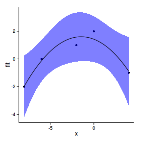
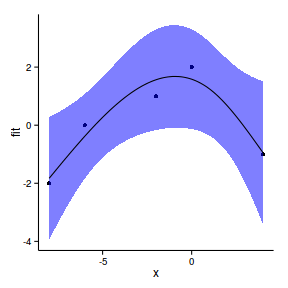
xs <- seq(min(data.s$x), max(data.s$x), l=100)
xmat <- model.matrix(~x, data.frame(x=xs))

mpred <- function(model, xmat, data.s) {
  pred <- as.vector(coef(model) %*% t(xmat))
  (se<-sqrt(diag(xmat %*% vcov(model) %*% t(xmat))))
  ci <- data.frame(pred+outer(se,qt(df=nrow(data.s)-2,c(.025,.975))))
  colnames(ci) <- c('lwr','upr')
  data.s.sum<-data.frame(pred, x=xs,se,ci)
  data.s.sum
}

data.s.sum<-mpred(data.s.glsExp, xmat, data.s)

plot(pred~x, ylim=c(min(lwr), max(upr)), data.s.sum, type="l")
lines(lwr~x, data.s.sum)
lines(upr~x, data.s.sum)
points(pred+residuals(data.s.glsExp)~x, data.s.sum)

newdata <- data.frame(x=xs)[1,]

Non-independence

one response is triggered by another
temporal/spatial autocorrelation
nested (hierarchical) design structures

Workshop 9.15a: Heterogeneity

Murray Logan

27-04-2014

Linear modelling assumptions

Linear modelling assumptions

Dealing with Heterogeneity

Dealing with Heterogeneity

Dealing with Heterogeneity

Dealing with Heterogeneity

Dealing with Heterogeneity

Dealing with Heterogeneity

Dealing with Heterogeneity

Dealing with Heterogeneity

Dealing with Heterogeneity

Dealing with Heterogeneity

Generalized least squares (GLS)

Generalized least squares (GLS)

Variance structures

Generalized least squares (GLS)

Generalized least squares (GLS)

wrong

Generalized least squares (GLS)

CORRECT

Generalized least squares (GLS)

Generalized least squares (GLS)

Generalized least squares (GLS)

Can we go better

Generalized least squares (GLS)

CORRECT

Generalized least squares (GLS)

Generalized least squares (GLS)

Generalized least squares (GLS)

Heteroscadacity in ANOVA

Heteroscadacity in ANOVA

Heteroscadacity in ANOVA

Heteroscadacity in ANOVA

Heteroscadacity in ANOVA

Heteroscadacity in ANOVA

Variance structures

Heteroscadacity in ANOVA

Heteroscadacity in ANOVA

Heteroscadacity in ANOVA

Heteroscadacity in ANOVA

Bayesian

Linear modelling assumptions

Non-independence

Variance-covariance

Compound symmetry

Temporal autocorrelation

Temporal autocorrelation

Temporal autocorrelation

Temporal autocorrelation

Temporal autocorrelation

Testing for autocorrelation

Residual plot

Testing for autocorrelation

Autocorrelation (acf) plot

First order autocorrelation (AR1)

First order auto-regressive (AR1)

First order auto-regressive (AR1)

First order auto-regressive (AR1)

First order auto-regressive (AR1)

First order auto-regressive (AR1)

First order auto-regressive (AR1)

Auto-regressive moving average (ARMA)

Summarize model

Bayesian

Spatial autocorrelation

Spatial autocorrelation

Spatial autocorrelation

Spatial autocorrelation

Detecting spatial autocorrelation

Bubble plot

Semi-variogram

Semi-variogram

Semi-variogram

Semi-variogram

Semi-variogram

Accommodating spatial autocorrelation

Accommodating spatial autocorrelation