Tutorial 10.6a - Poisson regression and log-linear models
05 Sep 2016
Poisson regression
Poisson regression is a type of generalized linear model (GLM) that models a positive integer (natural number) response against a linear predictor via a specific link function. The linear predictor is typically a linear combination of effects parameters (e.g. $\beta_0 + \beta_1x_x$). The role of the link function is to transform the expected values of the response y (which is on the scale of (0,$\infty$), as is the Poisson distribution from which expectations are drawn) into the scale of the linear predictor (which is $-\infty,\infty$).
Poisson regression is a type of generalized linear model (GLM) that models a positive integer (natural number) response against a linear predictor via a specific link function. The linear predictor is typically a linear combination of effects parameters (e.g. $\beta_0 + \beta_1x_x$). The role of the link function is to transform the expected values of the response y (which is on the scale of (0,$\infty$), as is the Poisson distribution from which expectations are drawn) into the scale of the linear predictor (which is $-\infty,\infty$).
As implied in the name of this group of analyses, a Poisson rather than Gaussian (normal) distribution is used to represent the errors (residuals). Like count data (number of individuals, species etc), the Poisson distribution encapsulates positive integers and is bound by zero at one end. Consequently, the degree of variability is directly related the expected value (equivalent to the mean of a Gaussian distribution). Put differently, the variance is a function of the mean. Repeated observations from a Poisson distribution located close to zero will yield a much smaller spread of observations than will samples drawn from a Poisson distribution located a greater distance from zero. In the Poisson distribution, the variance has a 1:1 relationship with the mean.
The canonical link function for the Poisson distribution is a log-link function.
Whilst the expectation that the mean=variance ($\mu=\sigma$) is broadly compatible with actual count data (that variance increases at the same rate as the mean), under certain circumstances, this might not be the case. For example, when there are other unmeasured influences on the response variable, the distribution of counts might be somewhat clumped which can result in higher than expected variability (that is $\sigma\gt\mu$). The variance increases more rapidly than does the mean. This is referred to as overdispersion. The degree to which the variability is greater than the mean (and thus the expected degree of variability) is called dispersion. Effectively, the Poisson distribution has a dispersion parameter (or scaling factor) of 1.
It turns out that overdispersion is very common for count data and it typically underestimates variability, standard errors and thus deflated p-values. There are a number of ways of overcoming this limitation, the effectiveness of which depend on the causes of overdispersion.
- Quasi-Poisson models - these introduce the dispersion parameter ($\phi$) into the model.
This approach does not utilize an underlying error distribution to calculate the maximum likelihood (there is no quasi-Poisson distribution).
Instead, if the Newton-Ralphson iterative reweighting least squares algorithm is applied using a direct specification of the relationship between
mean and variance ($var(y)=\phi\mu$), the estimates of the regression coefficients are identical to those of the maximum
likelihood estimates from the Poisson model. This is analogous to fitting ordinary least squares on symmetrical, yet not normally distributed data -
the parameter estimates are the same, however they won't necessarily be as efficient.
The standard errors of the coefficients are then calculated by multiplying the Poisson model coefficient
standard errors by $\sqrt{\phi}$.
Unfortunately, because the quasi-poisson model is not estimated via maximum likelihood, properties such as AIC and log-likelihood cannot be derived. Consequently, quasi-poisson and Poisson model fits cannot be compared via either AIC or likelihood ratio tests (nor can they be compared via deviance as uasi-poisson and Poisson models have the same residual deviance). That said, quasi-likelihood can be obtained by dividing the likelihood from the Poisson model by the dispersion (scale) factor.
- Negative binomial model - technically, the negative binomial distribution is a probability distribution for the number of successes before a specified number of failures.
However, the negative binomial can also be defined (parameterized) in terms of a mean ($\mu$) and scale factor ($\omega$),
$$p(y_i)=\frac{\Gamma(y_i+\omega)}{\Gamma(\omega)y!}\times\frac{\mu_i^{y_i}\omega^\omega}{(\mu_i+\omega)^{\mu_i+\omega}}$$
where the expectected value of the values $y_i$ (the means) are ($mu_i$) and the variance is $y_i=\frac{\mu_i+\mu_i^2}{\omega}$.
In this way, the negative binomial is a two-stage hierarchical process in which the response is modeled against a Poisson distribution whose expected count is in turn
modeled by a Gamma distribution with a mean of $\mu$ and constant scale parameter ($\omega$).
Strictly, the negative binomial is not an exponential family distribution (unless $\omega$ is fixed as a constant), and thus negative binomial models cannot be fit via the usual GLM iterative reweighting algorithm. Instead estimates of the regression parameters along with the scale factor ($\omega$) are obtained via maximum likelihood.
The negative binomial model is useful for accommodating overdispersal when it is likely caused by clumping (due to the influence of other unmeasured factors) within the response.
- Zero-inflated Poisson model - overdispersion can also be caused by the presence of a greater number of zero's than would otherwise be expected for a Poisson distribution.
There are potentially two sources of zero counts - genuine zeros and false zeros.
Firstly, there may genuinely be no individuals present. This would be the number expected by a Poisson distribution.
Secondly, individuals may have been present yet not detected or may not even been possible.
These are false zero's and lead to zero inflated data (data with more zeros than expected).
For example, the number of joeys accompanying an adult koala could be zero because the koala has no offspring (true zero) or because the koala is male or infertile (both of which would be examples of false zeros). Similarly, zero counts of the number of individual in a transect are due either to the absence of individuals or the inability of the observer to detect them. Whilst in the former example, the latent variable representing false zeros (sex or infertility) can be identified and those individuals removed prior to analysis, this is not the case for the latter example. That is, we cannot easily partition which counts of zero are due to detection issues and which are a true indication of the natural state.
Consistent with these two sources of zeros, zero-inflated models combine a binary logistic regression model (that models count membership according to a latent variable representing observations that can only be zeros - not detectable or male koalas) with a Poisson regression (that models count membership according to a latent variable representing observations whose values could be 0 or any positive integer - fertile female koalas).
Poisson regression
Scenario and Data
Lets say we wanted to model the abundance of an item ($y$) against a continuous predictor ($x$). As this section is mainly about the generation of artificial data (and not specifically about what to do with the data), understanding the actual details are optional and can be safely skipped. Consequently, I have folded (toggled) this section away.
- the sample size = 20
- the continuous $x$ variable is a random uniform spread of measurements between 1 and 20
- the rate of change in log $y$ per unit of $x$ (slope) = 0.1.
- the value of $x$ when log$y$ equals 0 (when $y$=1)
- to generate the values of $y$ expected at each $x$ value, we evaluate the linear predictor (created by calculating the outer product of the model matrix and the regression parameters). These expected values are then transformed into a scale mapped by (0,$\infty$) by using the log function $e^{linear~predictor}$
- finally, we generate $y$ values by using the expected $y$ values ($\lambda$) as probabilities when drawing random numbers from a Poisson distribution. This step adds random noise to the expected $y$ values and returns only 0's and positive integers.
set.seed(8)
#The number of samples
n.x <- 20
#Create x values that at uniformly distributed throughout the rate of 1 to 20
x <- sort(runif(n = n.x, min = 1, max =20))
mm <- model.matrix(~x)
intercept <- 0.6
slope=0.1
#The linear predictor
linpred <- mm %*% c(intercept,slope)
#Predicted y values
lambda <- exp(linpred)
#Add some noise and make binomial
y <- rpois(n=n.x, lambda=lambda)
dat <- data.frame(y,x)
data.pois <- dat
write.table(data.pois, file='../downloads/data/data.pois.csv', quote=F, row.names=F, sep=',')
With these sort of data, we are primarily interested in investigating whether there is a relationship between the positive integer response variable and the linear predictor (linear combination of one or more continuous or categorical predictors).
Exploratory data analysis and initial assumption checking
- All of the observations are independent - this must be addressed at the design and collection stages
- The response variable (and thus the residuals) should be matched by an appropriate distribution (in the case of positive integers response - a Poisson is appropriate).
- All observations are equally influential in determining the trends - or at least no observations are overly influential. This is most effectively diagnosed via residuals and other influence indices and is very difficult to diagnose prior to analysis
- the relationship between the linear predictor (right hand side of the regression formula) and the link function should be linear. A scatterplot with smoother can be useful for identifying possible non-linearity.
- The dispersion factor is close to 1
There are five main potential models we could consider fitting to these data:
- Ordinary least squares regression (general linear model) - assumes normality of residuals
- Poisson regression - assumes mean=variance (dispersion=1)
- Quasi-poisson regression - a general solution to overdispersion. Assumes variance is a function of mean, dispersion estimated, however likelihood based statistics unavailable
- Negative binomial regression - a specific solution to overdispersion caused by clumping (due to an unmeasured latent variable). Scaling factor ($\omega$) is estimated along with the regression parameters.
- Zero-inflation model - a specific solution to overdispersion caused by excessive zeros (due to an unmeasured latent variable). Mixture of binomial and Poisson models.
Confirm non-normality and explore clumping
When counts are all very large (not close to 0) and their ranges do not span orders of magnitude, they take on very Gaussian properties (symmetrical distribution and variance independent of the mean). Given that models based on the Gaussian distribution are more optimized and recognized than Generalized Linear Models, it can be prudent to adopt Gaussian models for such data. Hence it is a good idea to first explore whether a Poisson model is likely to be more appropriate than a standard Gaussian model.
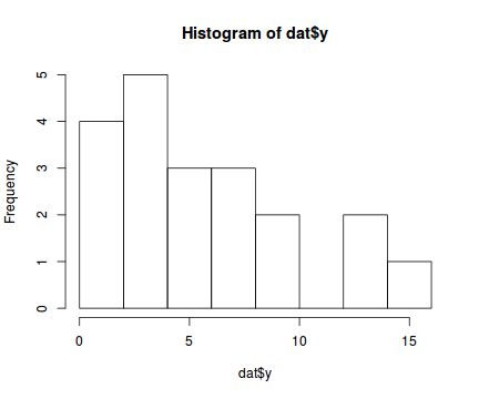
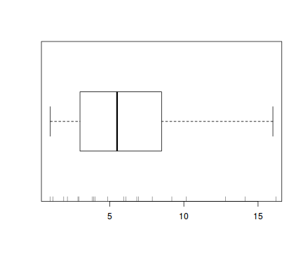
The potential for overdispersion can be explored by adding a rug to boxplot. The rug is simply tick marks on the inside of an axis at the position corresponding to an observation. As multiple identical values result in tick marks drawn over one another, it is typically a good idea to apply a slight amount of jitter (random displacement) to the values used by the rug.
hist(dat$y)
boxplot(dat$y, horizontal=TRUE)
rug(jitter(dat$y), side=1)
Confirm linearity
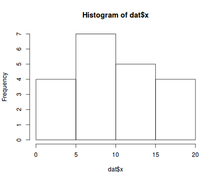
Lets now explore linearity by creating a histogram of the predictor variable ($x$) and a scatterplot of the relationship between the response ($y$) and the predictor ($x$)
hist(dat$x)
#now for the scatterplot
plot(y~x, dat, log="y")
with(dat, lines(lowess(y~x)))
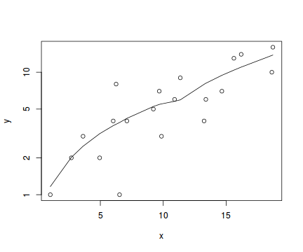
Conclusions: the predictor ($x$) does not display any skewness or other issues that might lead to non-linearity. The lowess smoother on the scatterplot does not display major deviations from a straight line and thus linearity is satisfied. Violations of linearity could be addressed by either:
- define a non-linear linear predictor (such as a polynomial, spline or other non-linear function)
- transform the scale of the predictor variables
Explore the distributional properties of the response
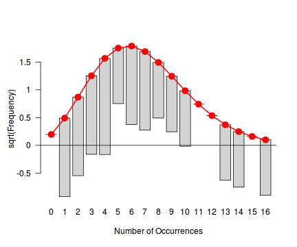
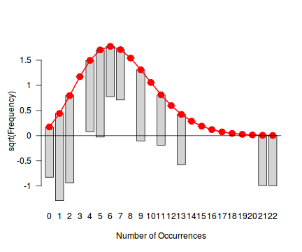
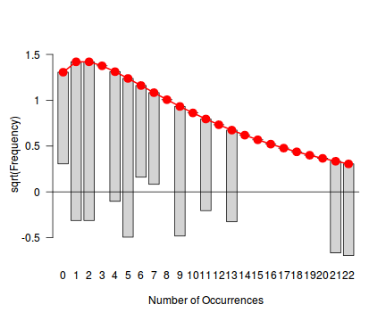
Tukey suggested a variation on a histogram for non-Gaussian distributions. His hanging rootogram features a frequency histogram (on a square-root scale) hanging from an equivalent reference distribution (such as a Poisson distribution). Apparently, the hanging nature makes it easier to detect deviations of the observed counts from the reference distribution (since the distribution will be curvilinear) and the square-root scale allows greater emphasis of smaller frequencies (since a histogram will normally be dominated by large frequencies).
The goodfit() and rootogram() functions in the vcd (Visualizing Categorical Data) package provide convenient ways of quickly exploring the broad suitability of Poisson, Binomial and Negative Binomial distributions to a response. Note however, these are of limited use on small (n<30) data sets and in the current case are only provided for illustrative purposes.
library(vcd)
fit <- goodfit(dat$y, type='poisson')
summary(fit)
	 Goodness-of-fit test for poisson distribution

                      X^2 df    P(> X^2)
Likelihood Ratio 25.33272 11 0.008146985
rootogram(fit)
fit <- goodfit(dat$y, type='nbinom')
summary(fit)
	 Goodness-of-fit test for nbinomial distribution

                      X^2 df  P(> X^2)
Likelihood Ratio 9.978856 10 0.4423503
rootogram(fit)
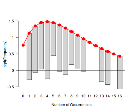
Conclusions - the goodness of fit and rootogram explorations suggest that a Negative Binomial is a good fit whereas the Poisson is less so (deviations of the observed counts from Poisson are greater than they from the Negative Binomial). However, this may well be as much of an artifact of the very small sample size as it is a genuine reflection of the most appropriate distribution against which to fit a model.
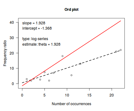
Ord demonstrated that the relationship between the ratio of predicted counts to predicted counts of previous bin ($k\frac{p_k}{p_{k-1}}$) and the count bins ($k$) followed a linear relationship for Poisson, Binomial, Negative Binomial and logarithmic series distributions (yet with different characteristic intercepts and slopes) and thus proposed a simple plot (Ord plot) for diagnosing appropriate discrete distributions. Ord indicated that parameters must be within a certain tolerance (nominally 0.1) of the defining coefficient to yield a conclusive diagnostic. The following table indicates the interpretation of Intercept and Slope parameters. Ord also suggested weighting the relationship by the square-root of the count frequencies so as to dampen fluctuations due to sampling variance. The table is also presented in order of testing - that is, first the routine tests whether a Poission is appropriate, if not, it explores a Binomial and so on.
| Intercept (a) | Slope (b) | Tolerance | Suggested Distribution (and parameters) | Estimated Parameter |
|---|---|---|---|---|
| + | 0 | abs(b)<tol | Poisson(λ) | λ=a |
| + | - | b<(-1*tol) | Binomial(n,p) | p = b/(b-1) |
| + | + | a<(-1*tol) | Negative Binomial(n,p) | p = 1-b |
| - | + | abs(a+b)< 4*tol | Logarithmic(θ) | θ = b θ = -a |
library(vcd)
Ord_plot(dat$y, tol=0.2)
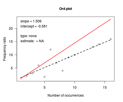
Conclusions- the small sample size makes this difficult to assess.
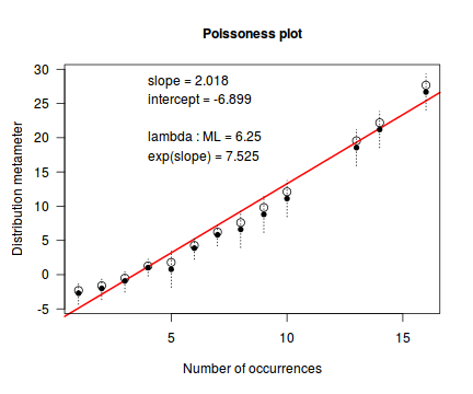
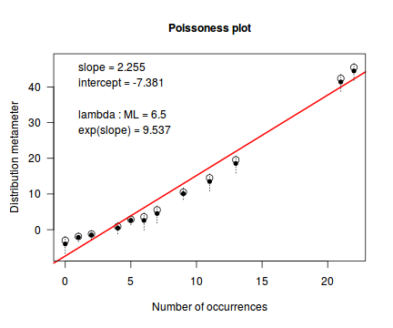
An alternative to the Ord plot is the robust distribution plot. Similar to a Q-Q normal plot, the robust distribution plot compares data to a reference distribution. Deviations from a straight line are indicative of a poor match between the data and the reference distribution. Open circles on the plot represent the observed count distribution metameter. Dotted lines and solid circles represent the 95% confidence intervals and centers thereof. Also provided on the plot are the coefficients (intercept and slope) of the relationship as well as the maximum likelihood estimates of the distribution parameters (Poisson: $\lambda$; Negative Binomial: $p$).
library(vcd)
distplot(dat$y, type='poisson')
distplot(dat$y, type="nbinom")
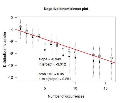
Conclusions - the data is a closer match to the Poisson distribution than the Negative Binomial distribution.
Explore zero inflation
Although we have already established that there are few zeros in the data (and thus overdispersion is unlikely to be an issue), we can also explore this by comparing the number of zeros in the data to the number of zeros that would be expected from a Poisson distribution with a mean equal to the mean count of the data.
#proportion of 0's in the data
dat.tab<-table(dat$y==0)
dat.tab/sum(dat.tab)
FALSE
    1
#proportion of 0's expected from a Poisson distribution
mu <- mean(dat$y)
cnts <- rpois(1000, mu)
dat.tab <- table(cnts == 0)
dat.tab/sum(dat.tab)
FALSE  TRUE
0.997 0.003
Model fitting or statistical analysis
We perform the Poisson regression using the glm() function. The most important (=commonly used) parameters/arguments for logistic regression are:
- formula: the linear model relating the response variable to the linear predictor
- family: specification of the error distribution (and link function).
Can be specified as either a string or as one of the family functions (which allows for the explicit declaration of the link function).
For examples:
- family="poisson" or equivalently family=poisson(link="log")
- data: the data frame containing the data
I will now fit the Poisson regression: $$log(\mu)=\beta_0+\beta_1x_1+\epsilon_i, \hspace{1cm}\epsilon\sim Poisson(\lambda)$$
dat.glm <- glm(y~x, data=dat, family="poisson")
Model evaluation
Prior to exploring the model parameters, it is prudent to confirm that the model did indeed fit the assumptions and was an appropriate fit to the data. There are a number of extractor functions (functions that extract or derive specific information from a model) available including:
| Extractor | Description |
|---|---|
| residuals() | Extracts the residuals from the model |
| fitted() | Extracts the predicted (expected) response values (on the link scale) at the observed levels of the linear predictor |
| predict() | Extracts the predicted (expected) response values (on either the link, response or terms (linear predictor) scale) |
| coef() | Extracts the model coefficients |
| deviance() | Extracts the deviance from the model |
| AIC() | Extracts the Akaike's Information Criterion from the model |
| AICc() | Extracts the Akaike's Information Criterion corrected for small sample sizes from the model (MuMIn package) |
| extractAIC() | Extracts the generalized Akaike's Information Criterion from the model |
| summary() | Summarizes the important output and characteristics of the model |
| anova() | Computes an analysis of deviance or log-likelihood ratio test (LRT) from the model |
| plot() | Generates a series of diagnostic plots from the model |
| effects() | Generates partial effects from fitted model (effects package) |
Lets explore the diagnostics - particularly the residuals
plot(dat.glm)
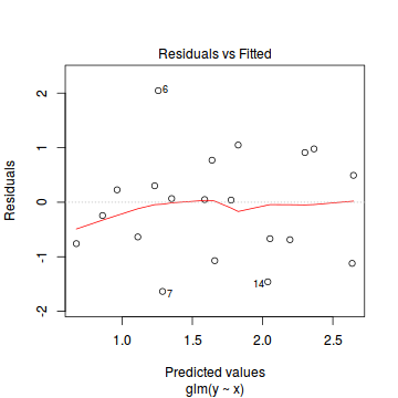
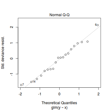
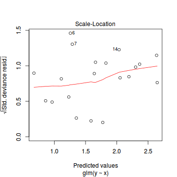
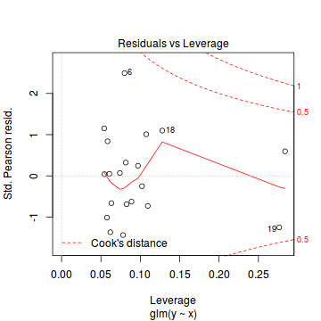
Unfortunately, unlike with linear models (Gaussian family), the expected distribution of data (residuals) varies over the range of fitted values for numerous (often competing) ways that make diagnosing (and attributing causes thereof) miss-specified generalized linear models from standard residual plots very difficult. The use of standardized (Pearson) residuals or deviance residuals can partly address this issue, yet they still do not offer completely consistent diagnoses across all issues (miss-specified model, over-dispersion, zero-inflation).
An alternative approach is to use simulated data from the fitted model to calculate an empirical cumulative density function from which residuals are are generated as values corresponding to the observed data along the density function. The (rather Bayesian) rationale is that if the model is correctly specified, then the observed data can be considered as a random draw from the fitted model. If this is the case, then residuals calculated from empirical cumulative density functions based on data simulated from the fitted model, should be totally uniform (flat) across the range of the linear predictor (fitted values) regardless of the model (Binomial, Poisson, linear, quadratic, hierarchical or otherwise). This uniformity can be explored by examining qq-plots (in which the trend should match a straight line) and plots of residual against the fitted values and each individual predictor (in which the noise should be uniform around zero across the range of x-values).
To illustrate this, lets generate 10 simulated data sets from our fitted model. This will generate a matrix with 10 columns and as many rows as there were in the original data. Think of it as 10 attempts to simulate the original data from the model.
dat.sim <- simulate(dat.glm, n=10)
dat.sim
   sim_1 sim_2 sim_3 sim_4 sim_5 sim_6 sim_7 sim_8 sim_9 sim_10
1      1     2     0     1     2     1     0     2     3      0
2      4     3     4     1     3     2     1     4     2      2
3      2     3     2     1     3     3     4     7     1      1
4      0     1     4     4     1     2     7     4     3      3
5      2    11     1     0     4     6     1     6     4      7
6      6     6     3     2     2     5     6     5     3      3
7      5     1     7     4     1     4     2     5     3      5
8      2     0     3     6     3     4     6     1     6      4
9      3     8     5     4     3     5     7     4     6      3
10     6     8     2     3     9     6     2     9     6      7
11     4     7     8     3     5     6     7     4     5      3
12     8     3     9     9     2     6    11    14     7      4
13     5     4     6     5     8     8     7     7     8      6
14     4     6     9    13     6     8     6    10    10      5
15     6     3     4     8    13     8     8     7     9      5
16    14    11     7    10     6    14     8     8    10     12
17     7     8    12     7    10    11     6     6    11      6
18    12     6    10     8    11    14    13    10    13     14
19    14    16    14    15    12    13     9    11    13     15
20    11    23     9     6    14    15    21     9    11      9
dat.sim <- simulate(dat.glm, n=250)
dat$y
[1] 1 2 3 2 4 8 1 4 5 7 3 6 9 4 6 7 13 14 10 16
par(mfrow=c(5,4), mar=c(3,3,1,1))
resid <- NULL
for (i in 1:nrow(dat.sim)) {
  e=data.matrix(dat.sim[i,])
  hist(e, main=i,las=1)
  resid[i] <- dat$y[i] - mean(e)
}
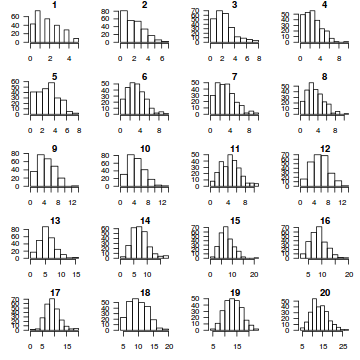
resid
 [1] -0.860 -0.432  0.252 -1.116  0.632  4.292 -2.656  0.168 -0.008  1.912 -2.032 -0.076  2.968
[14] -3.880 -1.804 -2.184  3.368  3.548 -3.992  2.060
resid <- NULL
for (i in 1:nrow(dat.sim)) {
  e=data.matrix(dat.sim[i,])
  d=density(e)
  plot(d, main=i,las=1)
  e=d$x[d$y==max(d$y)]
  resid[i] <- (dat$y[i]) - e
}
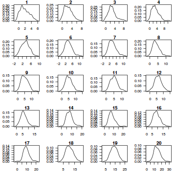
resid
 [1] -0.01423095  0.91310617  0.93170248 -0.95423394  0.11994091  4.84640620 -1.72654712  0.98374257
 [9]  1.48647220  3.00604679 -2.19419319 -0.65422933  3.54516521 -4.16700100 -0.96024660 -2.02230842
[17]  3.85646518  4.49531160 -4.09508226  4.42694204
par(mfrow=c(1,1))
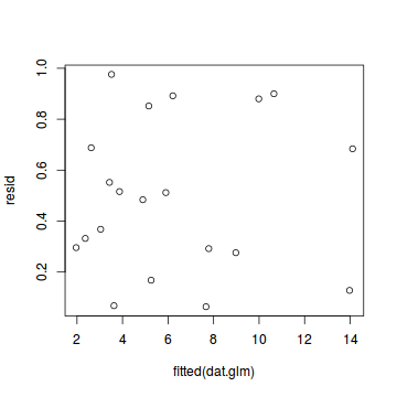
plot(resid~fitted(dat.glm))
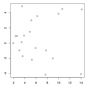
Now for each row of these simulated data, we calculate the empirical cumulative density function and use this function to predict new y-values (=residuals) corresponding to each observed y-value. Actually, 10 simulated samples is totally inadequate, we should use at least 250. I initially used 10, just so we could explore the output. We will re-simulate 250 times. Note also, for integer responses (including binary), uniform random noise is added to both the simulated and observed data so that we can sensibly explore zero inflation. The resulting residuals will be on a scale from 0 to 1 and therefore the residual plot should be centered around a y-value of 0.5.
dat.sim <- simulate(dat.glm, n=250)
par(mfrow=c(5,4), mar=c(3,3,1,1))
resid <- NULL
for (i in 1:nrow(dat.sim)) {
  e=ecdf(data.matrix(dat.sim[i,] + runif(250, -0.5, 0.5)))
  plot(e, main=i,las=1)
  resid[i] <- e(dat$y[i] + runif(250, -0.5, 0.5))
}
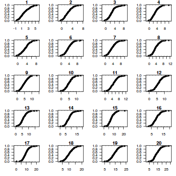
resid
 [1] 0.296 0.332 0.688 0.368 0.552 0.976 0.068 0.516 0.484 0.852 0.168 0.512 0.892 0.064 0.292 0.276
[17] 0.880 0.900 0.128 0.684
plot(resid ~ fitted(dat.glm))
The DHARMa package provides a number of convenient routines to explore standardized residuals simulated from fitted models based on the concepts outlined above. Along with generating simulated residuals, simple qq plots and residual plots are available. By default, the residual plots include quantile regression lines (0.25, 0.5 and 0.75), each of which should be straight and flat.
- in overdispersed models, the qq trend will deviate substantially from a straight line
- non-linear models will display trends in the residuals
library(DHARMa)
dat.sim <- simulateResiduals(dat.glm)
dat.sim
[1] "Class DHARMa with simulated residuals based on 250 simulations with refit = FALSE"
[1] "see ?DHARMa::simulateResiduals for help"
[1] "-----------------------------"
 [1] 0.228 0.628 0.580 0.316 0.536 0.980 0.100 0.544 0.496 0.760 0.124 0.532 0.864 0.052 0.288 0.304
[17] 0.816 0.800 0.124 0.656
plotSimulatedResiduals(dat.sim)
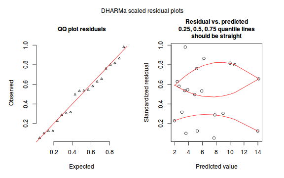
Conclusions: there is no obvious patterns in the qq-plot or residuals, or at least there are no obvious trends remaining that would be indicative of overdispersion or non-linearity.
Goodness of fit of the model
We can also explore the goodness of the fit of the model via:
- Pearson's $\chi^2$ residuals
- explores whether there are any significant patterns remaining in the residuals
dat.resid <- sum(resid(dat.glm, type = "pearson")^2)
1 - pchisq(dat.resid, dat.glm$df.resid)
[1] 0.4896553
- Deviance ($G^2$) - similar to the $\chi^2$ test above, yet uses deviance
1-pchisq(dat.glm$deviance, dat.glm$df.resid)
[1] 0.5076357
- The DHARMa package also has a routine for running a Kologorov-Smirnov test test to explore overall uniformity of the residuals as a goodness-of-fit test on the scaled residuals.
Conclusions: neither Pearson residuals, Deviance or Kolmogorov-Smirnov test of uniformity indicate a lack of fit (p values greater than 0.05)testUniformity(dat.sim)
	One-sample Kolmogorov-Smirnov test

data:  simulationOutput$scaledResiduals
D = 0.096, p-value = 0.9928
alternative hypothesis: two-sided
In this demonstration we fitted the Poisson model. We could also compare (using AIC or deviance) its fit to that of a Gaussian model.
Conclusions: from the perspective of both AIC and deviance, the Poisson model would be considered a better fit to the data.dat.glmG <- glm(y~x, data=dat, family="gaussian") AIC(dat.glm, dat.glmG)
Error in AIC.glm(dat.glm, dat.glmG): unused argument (dat.glmG)
#Poisson deviance
dat.glm$deviance
[1] 17.2258
#Gaussian deviance
dat.glmG$deviance
[1] 118.1146
Dispersion
Recall that the Poisson regression model assumes that variance=mean ($var=\mu\phi$ where $\phi=1$) and thus dispersion ($\phi=\frac{var}{\mu}=1$). However, we can also calculate approximately what the dispersion factor would be by using the model deviance as a measure of variance and the model residual degrees of freedom as a measure of the mean (since the expected value of a Poisson distribution is the same as its degrees of freedom). $$\phi=\frac{Deviance}{df}$$
Conclusion: the estimated dispersion parameter is very close to 1 thereby confirming that overdispersion is unlikely to be an issue.dat.glm$deviance/dat.glm$df.resid
[1] 0.9569887
#Or alternatively, via Pearson's residuals
Resid <- resid(dat.glm, type = "pearson")
sum(Resid^2) / (nrow(dat) - length(coef(dat.glm)))
[1] 0.9716981
The DHARMa package also provides elegant ways to explore overdispersion, zero-inflation (and spatial and temporal autocorrelation). For these methods, the model is repeatedly refit with the simulated data to yield bootstrapped refitted residuals. The test for overdispersion compares the approximate deviances of the observed model with the those of the simulated models.
Conclusions: there is no evidence of overdispersion nor zero-inflation.testOverdispersion(simulateResiduals(dat.glm, refit=T))
	Overdispersion test via comparison to simulation under H0

data:  simulateResiduals(dat.glm, refit = T)
dispersion = 0.95895, p-value = 0.472
alternative hypothesis: overdispersion
testZeroInflation(simulateResiduals(dat.glm, refit=T))
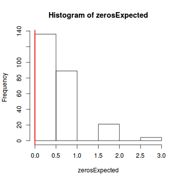
	Zero-inflation test via comparison to expected zeros with simulation under H0

data:  simulateResiduals(dat.glm, refit = T)
ratioObsExp = 0, p-value = 0.456
alternative hypothesis: more
The AER package includes a dispersiontest() function which takes a slightly different approach. In its simplest form, the dispersiontest() function considers variance as equal to: $$ var(y) = \mu + \alpha \times \mu $$ if $\alpha < 0$, the model is underdispersed and if $\alpha > 0$, the model is overdispersed. $\alpha$ is estimated via auxillary OLS regression and tested against a null hypothesis of $\alpha = 0$. Dispersion is also estimated according to: $$ \phi = \alpha + 1 $$
Conclusions - there is no evidence that the model is overdispersed. If anything it is slightly underdispersed (however as this is a very small fabricated data set, such underdispersion is likely to be an artifact)library(AER) dispersiontest(dat.glm)
	Overdispersion test

data:  dat.glm
z = -0.4719, p-value = 0.6815
alternative hypothesis: true dispersion is greater than 1
sample estimates:
dispersion
 0.8813912
Comparing fitted values to observed counts
Whilst it does not necessarily stand that a model that can accurately predict the training data is a good model, it is true that a model that cannot predict the training data is unlikely to be a good model. Therefore if there is not a reasonably good relationship between the fitted values against the observed values, it is likely that our model is ill-defined or inadequate in some way.
tempdata <- data.frame(obs=dat$y, fitted=fitted(dat.glm))
library(ggplot2)
ggplot(tempdata, aes(y=fitted, x=obs)) + geom_point()
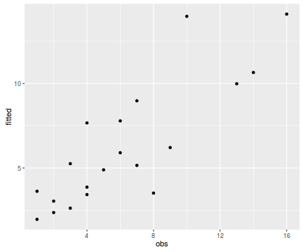
Conclusions - the relationship between fitted values and observed counts is reasonably good. There is nothing to suggest that the model is grossly inadequate etc.
Exploring the model parameters, test hypotheses
If there was any evidence that the assumptions had been violated or the model was not an appropriate fit, then we would need to reconsider the model and start the process again. In this case, there is no evidence that the test will be unreliable so we can proceed to explore the test statistics. The main statistic of interest is the Wald statistic ($z$) for the slope parameter.
summary(dat.glm)
Call:
glm(formula = y ~ x, family = "poisson", data = dat)

Deviance Residuals:
    Min       1Q   Median       3Q      Max
-1.6353  -0.7049   0.0440   0.5624   2.0457

Coefficients:
            Estimate Std. Error z value Pr(>|z|)
(Intercept)  0.56002    0.25395   2.205   0.0274 *
x            0.11151    0.01858   6.000 1.97e-09 ***
---
Signif. codes:  0 '***' 0.001 '**' 0.01 '*' 0.05 '.' 0.1 ' ' 1

(Dispersion parameter for poisson family taken to be 1)

    Null deviance: 55.614  on 19  degrees of freedom
Residual deviance: 17.226  on 18  degrees of freedom
AIC: 90.319

Number of Fisher Scoring iterations: 4
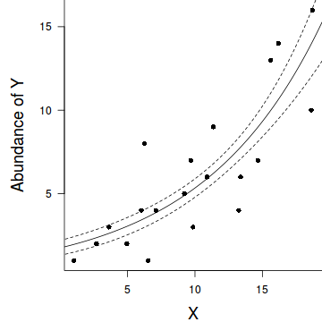
Conclusions: We would reject the null hypothesis (p<0.05). An increase in x is associated with a significant linear increase (positive slope) in log $y$ abundance. Every 1 unit increase in $x$ is associated with a 0.1115 unit increase in $\log y$ abundance We usually express this in terms of $y$ than $\log y$, so every 1 unit increase in $x$ is associated with a ($e^{0.1115}=1.12$) 1.12 unit increase in $y$ abundance.
P-values are widely acknowledged as a rather flawed means of inference testing (as in hypothesis testing in general). An alternate way of exploring the characteristics of parameter estimates is to calculate their confidence intervals. Confidence intervals that do not overlap with the null hypothesis parameter value (e.g. effect of 0), are an indication of a significant effect. Recall however, that in frequentist statistics the confidence intervals are interpreted as the range of values that are likely to contain the true mean on 95 out of 100 (95%) repeated samples.
Conclusions: A 1 unit increase in $x$ is associated with a ($e^{0.1115}=1.12$) 1.12 (1.08,1.16) unit increase in $y$ abundance.library(gmodels) ci(dat.glm)
             Estimate   CI lower  CI upper Std. Error      p-value
(Intercept) 0.5600204 0.02649343 1.0935474 0.25394898 2.743671e-02
x           0.1115114 0.07246668 0.1505562 0.01858457 1.970579e-09
Further explorations of the trends
A measure of the strength of the relationship can be obtained according to: $$quasi R^2 = 1-\left(\frac{deviance}{null~deviance}\right)$$
Conclusions: approximately1-(dat.glm$deviance/dat.glm$null)
[1] 0.6902629
69% of the variability in abundance can be explained by its relationship to $x$. Technically, it is69% of the variability in $\log y$ (the link function) is explained by its relationship to $x$.Finally, we will create a summary plot.
par(mar = c(4, 5, 0, 0))
plot(y ~ x, data = dat, type = "n", ann = F, axes = F)
points(y ~ x, data = dat, pch = 16)
xs <- seq(0, 20, l = 1000)
ys <- predict(dat.glm, newdata = data.frame(x = xs), type = "response", se = T)
points(ys$fit ~ xs, col = "black", type = "l")
lines(ys$fit - 1 * ys$se.fit ~ xs, col = "black", type = "l", lty = 2)
lines(ys$fit + 1 * ys$se.fit ~ xs, col = "black", type = "l", lty = 2)
axis(1)
mtext("X", 1, cex = 1.5, line = 3)
axis(2, las = 2)
mtext("Abundance of Y", 2, cex = 1.5, line = 3)
box(bty = "l")
Quasi-Poisson regression
Lets say we wanted to model the abundance of an item ($y$) against a continuous predictor ($x$). As this section is mainly about the generation of artificial data (and not specifically about what to do with the data), understanding the actual details are optional and can be safely skipped. Consequently, I have folded (toggled) this section away.
Random data incorporating the following trends (effect parameters)- define a function that will generate random samples from a quasi-poisson distribution $$QuasiPoisson\left(\frac{\mu}{\phi-1}, \frac{1}{\phi}\right)$$ where $\mu$ is the expected value (mean) and $\phi$ is the dispersion factor such that $var(y)=\phi\mu$.
- the sample size = 20
- the continuous $x$ variable is a random uniform spread of measurements between 1 and 20
- the rate of change in log $y$ per unit of $x$ (slope) = 0.1.
- the value of $x$ when log$y$ equals 0 (when $y$=1)
- to generate the values of $y$ expected at each $x$ value, we evaluate the linear predictor (created by calculating the outer product of the model matrix and the regression parameters). These expected values are then transformed into a scale mapped by (0,$\infty$) by using the log function $e^{linear~predictor}$
- finally, we generate $y$ values by using the expected $y$ values ($\lambda$) as probabilities when drawing random numbers from a quasi-poisson distribution. This step adds random noise to the expected $y$ values and returns only 0's and positive integers.
#Quasi-poisson distrition
rqpois <- function(n, lambda, phi) {
  mu = lambda
  r = rnbinom(n, size=mu/phi/(1-1/phi),prob=1/phi)
  return(r)
}

set.seed(8)
#The number of samples
n.x <- 20
#Create x values that at uniformly distributed throughout the rate of 1 to 20
x <- sort(runif(n = n.x, min = 1, max =20))
mm <- model.matrix(~x)
intercept <- 0.6
slope=0.1
#The linear predictor
linpred <- mm %*% c(intercept,slope)
#Predicted y values
lambda <- exp(linpred)
#Add some noise and make binomial
y <- rqpois(n=n.x, lambda=lambda, phi=4)
dat.qp <- data.frame(y,x)
data.qp <- dat.qp
write.table(data.qp, file='../downloads/data/data.qp.csv', quote=F, row.names=F, sep=',')
Exploratory data analysis and initial assumption checking
The assumptions are:- All of the observations are independent - this must be addressed at the design and collection stages
- The response variable (and thus the residuals) should be matched by an appropriate distribution (in the case of positive integers response - a Poisson is appropriate).
- All observations are equally influential in determining the trends - or at least no observations are overly influential. This is most effectively diagnosed via residuals and other influence indices and is very difficult to diagnose prior to analysis
- the relationship between the linear predictor (right hand side of the regression formula) and the link function should be linear. A scatterplot with smoother can be useful for identifying possible non-linearity.
- Dispersion is either 1 or overdispersion is accounted for in the model and is not due to excessive clumping or zero-inflation
Recall from Poisson regression, there are five main potential models that we could consider fitting to these data.
There are five main potential models we could consider fitting to these data:
- Ordinary least squares regression (general linear model) - assumes normality of residuals
- Poisson regression - assumes mean=variance (dispersion=1)
- Quasi-poisson regression - a general solution to overdispersion. Assumes variance is a function of mean, dispersion estimated, however likelihood based statistics unavailable
- Negative binomial regression - a specific solution to overdispersion caused by clumping (due to an unmeasured latent variable). Scaling factor ($\omega$) is estimated along with the regression parameters.
- Zero-inflation model - a specific solution to overdispersion caused by excessive zeros (due to an unmeasured latent variable). Mixture of binomial and Poisson models.
Confirm non-normality and explore clumping
Check the distribution of the $y$ abundances
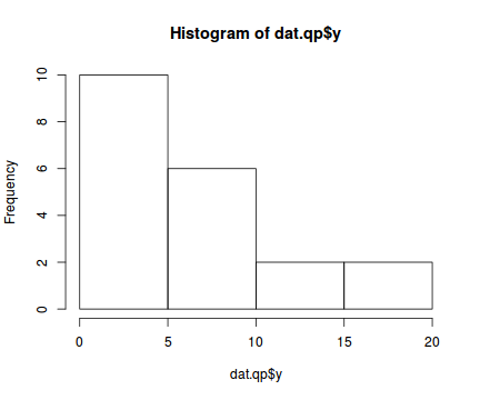
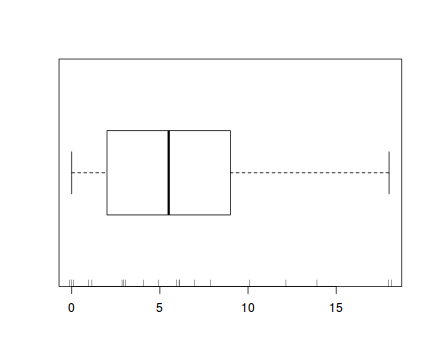
There is definitely signs of non-normality that would warrant some form of Poisson model. There is also some evidence of clumping that might result in overdispersion. Some zero values are present, yet there are not so many that we would be concerned about zero-inflation.hist(dat.qp$y)
boxplot(dat.qp$y, horizontal=TRUE)
rug(jitter(dat.qp$y), side=1)
Confirm linearity
Lets now explore linearity by creating a histogram of the predictor variable ($x$) and a scatterplot of the relationship between the response ($y$) and the predictor ($x$)
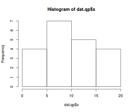
hist(dat.qp$x)
#now for the scatterplot
plot(y~x, dat.qp, log="y")
with(dat.qp, lines(lowess(y~x)))
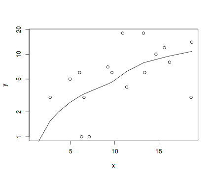
Conclusions: the predictor ($x$) does not display any skewness or other issues that might lead to non-linearity. The lowess smoother on the scatterplot does not display major deviations from a straight line and thus linearity is satisfied. Violations of linearity could be addressed by either:
- define a non-linear linear predictor (such as a polynomial, spline or other non-linear function)
- transform the scale of the predictor variables
Explore the distributional properties of the response
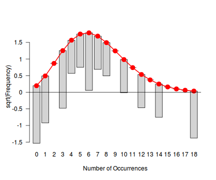
Tukey suggested a variation on a histogram for non-Gaussian distributions. His hanging rootogram features a frequency histogram (on a square-root scale) hanging from an equivalent reference distribution (such as a Poisson distribution). Apparently, the hanging nature makes it easier to detect deviations of the observed counts from the reference distribution (since the distribution will be curvilinear) and the square-root scale allows greater emphasis of smaller frequencies (since a histogram will normally be dominated by large frequencies).
The goodfit() and rootogram() functions in the vcd (Visualizing Categorical Data) package provide convenient ways of quickly exploring the broad suitability of Poisson, Binomial and Negative Binomial distributions to a response. Note however, these are of limited use on small (n<30) data sets and in the current case are only provided for illustrative purposes.
library(vcd)
fit <- goodfit(dat.qp$y, type='poisson')
summary(fit)
Goodness-of-fit test for poisson distribution X^2 df P(> X^2) Likelihood Ratio 67.9097 10 1.12105e-10rootogram(fit)
fit <- goodfit(dat.qp$y, type='nbinom')
summary(fit)
Goodness-of-fit test for nbinomial distribution X^2 df P(> X^2) Likelihood Ratio 21.60097 9 0.01023342rootogram(fit)
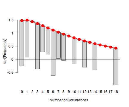
Conclusions - the goodness of fit and rootogram explorations suggest that a Poisson distribution is not a good fit. Potentially, a Negative Binomial is a better choice, although again, small sample sizes will hinder the usefulness of this diagnostic.
As an alternative, lets explore the Ord and robust distribution plots
library(vcd)
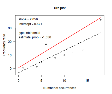
Ord_plot(dat.qp$y, tol=0.1)
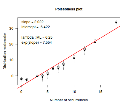
distplot(dat.qp$y, type='poisson')
distplot(dat.qp$y, type="nbinom")
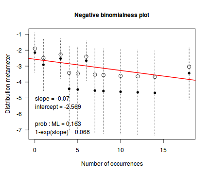
Conclusions - the Ord plot recommends a Negative Binomial. The Poissoness plot does show some evidence of curvilinearity (if that is indeed a word!). Not that the Negative binomialness plot is much better.
Explore zero inflation
Although we have already established that there are few zeros in the data (and thus overdispersion is unlikely to be an issue), we can also explore this by comparing the number of zeros in the data to the number of zeros that would be expected from a Poisson distribution with a mean equal to the mean count of the data.
In the above, the value under FALSE is the proportion of non-zero values in the data and the value under TRUE is the proportion of zeros in the data. In this example, there appears to be a higher proportion of zeros than would be expected. However, if we consider the small sample size of the observed data ($n=20$), there are still only a small number of zeros (#proportion of 0's in the data dat.qp.tab<-table(dat.qp$y==0) dat.qp.tab/sum(dat.qp.tab)
FALSE  TRUE
 0.85  0.15
#proportion of 0's expected from a Poisson distribution
mu <- mean(dat.qp$y)
cnts <- rpois(1000, mu)
dat.qp.tabE <- table(cnts == 0)
dat.qp.tabE/sum(dat.qp.tabE)
FALSE  TRUE
0.997 0.003
3). Nevertheless, a slight excess of zeros might also contribute to overdispersion.Model fitting or statistical analysis
A number of properties of the data during exploratory data analysis have suggested that overdispersion could be an issue. There is a hint of clumping of the response variable and there are also more zeros than we might have expected. At this point, we could consider which of these issues were likely to most severely impact on the fit of the models (clumping or excessive zeros) and fit a model that specifically addresses the issue (negative binomial, zero-inflated Poisson or even zero-inflated binomial). Alternatively, we could perform the Quasi-Poisson regression (which is a more general approach) using the glm() function. The most important (=commonly used) parameters/arguments for logistic regression are:
- formula: the linear model relating the response variable to the linear predictor
- family: specification of the error distribution (and link function).
Can be specified as either a string or as one of the family functions (which allows for the explicit declaration of the link function).
For examples:
- family="quasipoisson" or equivalently family=quasipoisson(link="log")
- data: the data frame containing the data
I will now fit the Quasi-Poisson regression: $$log(\mu)=\beta_0+\beta_1x_1+\epsilon_i, \hspace{1cm}var(y)=\omega\mu$$
dat.qp.glm <- glm(y~x, data=dat.qp, family="quasipoisson")
Model evaluation
Prior to exploring the model parameters, it is prudent to confirm that the model did indeed fit the assumptions and was an appropriate fit to the data. There are a number of extractor functions (functions that extract or derive specific information from a model) available including:
Extractor Description residuals() Extracts the residuals from the model fitted() Extracts the predicted (expected) response values (on the link scale) at the observed levels of the linear predictor predict() Extracts the predicted (expected) response values (on either the link, response or terms (linear predictor) scale) coef() Extracts the model coefficients deviance() Extracts the deviance from the model summary() Summarizes the important output and characteristics of the model anova() Computes an analysis of deviance or log-likelihood ratio test (LRT) from the model plot() Generates a series of diagnostic plots from the model Lets explore the diagnostics - particularly the residuals
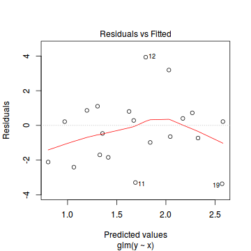
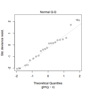
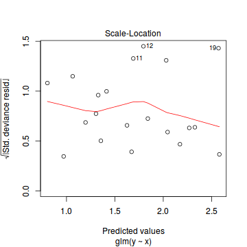
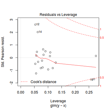
Conclusions: there is no obvious patterns in the residuals, or at least there are no obvious trends remaining that would be indicative of non-linearity. None of the observations are considered overly influential (Cooks' D values not approaching 1).plot(dat.qp.glm)
Since the regression coefficients are estimated directly from maximum likelihood without taking into account an error distribution, genuine log-likelihoods are not calculated. Consequently, derived model comparison metrics such as AIC are not formally available. Furthermore, as both Poisson and Quasi-Poisson models yield identical deviance, we cannot compare the fit of the quasi-poisson to a Poisson model via deviance either
dat.p.glm <- glm(y~x, data=dat.qp, family="poisson")
#Poisson deviance
dat.p.glm$deviance
[1] 69.98741
#Quasi-poisson deviance
dat.qp.glm$deviance
[1] 69.98741
tempdata <- data.frame(obs=dat.qp$y, fitted=fitted(dat.qp.glm))
library(ggplot2)
ggplot(tempdata, aes(y=fitted, x=obs)) + geom_point()
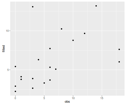
Conclusions - the relationship between fitted values and observed counts is ok without being great. There are clearly a few observations for which the model in very inaccurate.
Exploring the model parameters, test hypotheses
If there was any evidence that the assumptions had been violated or the model was not an appropriate fit, then we would need to reconsider the model and start the process again. In this case, there is no evidence that the test will be unreliable so we can proceed to explore the test statistics. The main statistic of interest is the t-statistic ($t$) for the slope parameter.
summary(dat.qp.glm)
Call:
glm(formula = y ~ x, family = "quasipoisson", data = dat.qp)

Deviance Residuals:
    Min       1Q   Median       3Q      Max
-3.3665  -1.7360  -0.1239   0.7436   3.9335

Coefficients:
            Estimate Std. Error t value Pr(>|t|)
(Intercept)   0.6996     0.4746   1.474   0.1577
x             0.1005     0.0353   2.846   0.0107 *
---
Signif. codes:  0 '***' 0.001 '**' 0.01 '*' 0.05 '.' 0.1 ' ' 1

(Dispersion parameter for quasipoisson family taken to be 3.698815)

    Null deviance: 101.521  on 19  degrees of freedom
Residual deviance:  69.987  on 18  degrees of freedom
AIC: NA

Number of Fisher Scoring iterations: 5
Conclusions: Note the dispersion (scale) factor is estimated as 3.699. Whilst this is greater than zero (thus confirming overdispersion), it would not be considered a large degree of overdispersion. So although negative binomial and zero-inflation models are typically preferred over Quasi-Poisson models (as they address the causes of overdispersion more directly), in this case, it is unlikely to make much difference.
We would reject the null hypothesis (p<0.05). An increase in x is associated with a significant linear increase (positive slope) in log $y$ abundance. Every 1 unit increase in $x$ is associated with a 0.1005 unit increase in $\log y$ abundance We usually express this in terms of $y$ than $\log y$, so every 1 unit increase in $x$ is associated with a ($e^{0.1}=1.11$) 1.11 unit increase in $y$ abundance.
P-values are widely acknowledged as a rather flawed means of inference testing (as in hypothesis testing in general). An alternate way of exploring the characteristics of parameter estimates is to calculate their confidence intervals. Confidence intervals that do not overlap with the null hypothesis parameter value (e.g. effect of 0), are an indication of a significant effect. Recall however, that in frequentist statistics the confidence intervals are interpreted as the range of values that are likely to contain the true mean on 95 out of 100 (95%) repeated samples.
Conclusions: A 1 unit increase in $x$ is associated with a ($e^{0.1005}=1.11$) 1.11 (1.03,1.19) unit increase in $y$ abundance.library(gmodels) ci(dat.qp.glm)
             Estimate    CI lower  CI upper Std. Error    p-value
(Intercept) 0.6996503 -0.29743825 1.6967388 0.47459569 0.15770206
x           0.1004823  0.02631858 0.1746461 0.03530057 0.01071259
Note that if we compare the Quasi-poisson parameter estimates to those of a Poisson, they have identical point estimates yet the Quasi-poisson model yields wider standard errors and confident intervals reflecting the greater variability modeled. In fact, the standard error of the Quasi-poisson model regression coefficients will be $\sqrt{\phi}$ times greater than those of the Poisson model. ($0.035 = \sqrt{3.699}\times 0.0184$).
summary(dat.p.glm<-glm(y~x,data=dat.qp, family="poisson"))
Call: glm(formula = y ~ x, family = "poisson", data = dat.qp) Deviance Residuals: Min 1Q Median 3Q Max -3.3665 -1.7360 -0.1239 0.7436 3.9335 Coefficients: Estimate Std. Error z value Pr(>|z|) (Intercept) 0.69965 0.24677 2.835 0.00458 ** x 0.10048 0.01835 5.474 4.39e-08 *** --- Signif. codes: 0 '***' 0.001 '**' 0.01 '*' 0.05 '.' 0.1 ' ' 1 (Dispersion parameter for poisson family taken to be 1) Null deviance: 101.521 on 19 degrees of freedom Residual deviance: 69.987 on 18 degrees of freedom AIC: 134.88 Number of Fisher Scoring iterations: 5ci(dat.p.glm)
             Estimate   CI lower  CI upper Std. Error      p-value
(Intercept) 0.6996503 0.18120562 1.2180949 0.24677006 4.579247e-03
x           0.1004823 0.06192025 0.1390444 0.01835483 4.389110e-08
Further explorations of the trends
A measure of the strength of the relationship can be obtained according to: $$quasi R^2 = 1-\left(\frac{deviance}{null~deviance}\right)$$
Conclusions: approximately1-(dat.qp.glm$deviance/dat.qp.glm$null)
[1] 0.310614
31.1% of the variability in abundance can be explained by its relationship to $x$. Technically, it is31.1% of the variability in $\log y$ (the link function) is explained by its relationship to $x$.Finally, we will create a summary plot.
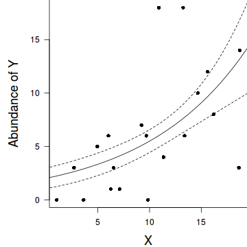
par(mar = c(4, 5, 0, 0))
plot(y ~ x, data = dat.qp, type = "n", ann = F, axes = F)
points(y ~ x, data = dat.qp, pch = 16)
xs <- seq(0, 20, l = 1000)
ys <- predict(dat.qp.glm, newdata = data.frame(x = xs), type = "response", se = T)
points(ys$fit ~ xs, col = "black", type = "l")
lines(ys$fit - 1 * ys$se.fit ~ xs, col = "black", type = "l", lty = 2)
lines(ys$fit + 1 * ys$se.fit ~ xs, col = "black", type = "l", lty = 2)
axis(1)
mtext("X", 1, cex = 1.5, line = 3)
axis(2, las = 2)
mtext("Abundance of Y", 2, cex = 1.5, line = 3)
box(bty = "l")
Observation-level random effect
One of the 'causes' of an overdispersed model is that important unmeasured (latent) effect(s) have not been incorporated. That is, there are one or more unobserved influences that result in a greater amount of variability in the response than would be expected from the Poisson distribution. We could attempt to 'mop up' this addition variation by adding a latent effect as a observation-level random effect in the model.
This random effect is just a numeric vector containing a sequence of integers from 1 to the number of observations. It acts as a proxy for the latent effects.
We will use the same data as the previous section on Quasipoisson to demonstrate observation-level random effects. Consequently, the exploratory data analysis section is the same as above (and therefore not repeated here).
Model fitting or statistical analysis
In order to incorporate observation-level random effects, we must use generalized linear mixed effects modelling. For this example, we will use the lme() function of the nlme package. The most important (=commonly used) parameters/arguments for logistic regression are:
- fixed: the linear model relating the response variable to the fixed component of the linear predictor
- random: the linear model relating the response variable to the random component of the linear predictor
- family: specification of the error distribution (and link function).
Can be specified as either a string or as one of the family functions (which allows for the explicit declaration of the link function).
For examples:
- family="poisson" or equivalently family=poisson(link="log")
- data: the data frame containing the data
I will now fit the observation-level random effects Poisson regression: $$log(\mu)=\beta_0+\beta_1x_1+Z\beta_2+\epsilon_i, \hspace{1cm}var(y)=\omega\mu$$
dat.qp$units <- 1:nrow(dat.qp)
library(MASS)
dat.qp.glmm <- glmmPQL(y~x, random=~1|units, data=dat.qp, family="poisson")
#OR
library(lme4)
dat.qp.glmer <- glmer(y~x+(1|units), data=dat.qp, family="poisson")
Model evaluation
Prior to exploring the model parameters, it is prudent to confirm that the model did indeed fit the assumptions and was an appropriate fit to the data. There are a number of extractor functions (functions that extract or derive specific information from a model) available including:
Extractor Description residuals() Extracts the residuals from the model fitted() Extracts the predicted (expected) response values (on the link scale) at the observed levels of the linear predictor predict() Extracts the predicted (expected) response values (on either the link, response or terms (linear predictor) scale) coef() Extracts the model coefficients fixef() Extracts the model coefficients of the fixed components ranef() Extracts the model coefficients of the fixed components deviance() Extracts the deviance from the model summary() Summarizes the important output and characteristics of the model anova() Computes an analysis of deviance or log-likelihood ratio test (LRT) from the model plot() Generates a series of diagnostic plots from the model Lets explore the diagnostics - particularly the residuals
plot(dat.qp.glmm)
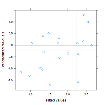
dat.qp.resid <- sum(resid(dat.qp.glmm, type = "pearson")^2)
1-pchisq(dat.qp.resid, dat.qp.glmm$fixDF$X[2])
[1] 0.703327
Conclusions:library(DHARMa) dat.qp.glmer.sim <- simulateResiduals(dat.qp.glmer) plotSimulatedResiduals(dat.qp.glmer.sim)
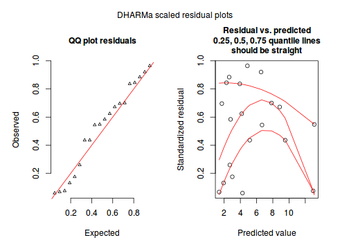
testUniformity(dat.qp.glmer.sim)
	One-sample Kolmogorov-Smirnov test

data:  simulationOutput$scaledResiduals
D = 0.144, p-value = 0.8013
alternative hypothesis: two-sided
dat.qp.glmer.sim <- simulateResiduals(dat.qp.glmer, refit=T)
testOverdispersion(dat.qp.glmer.sim)
	Overdispersion test via comparison to simulation under H0

data:  dat.qp.glmer.sim
dispersion = 0.97779, p-value = 0.412
alternative hypothesis: overdispersion
testZeroInflation(dat.qp.glmer.sim)
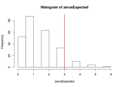
	Zero-inflation test via comparison to expected zeros with simulation under H0

data:  dat.qp.glmer.sim
ratioObsExp = 1.9841, p-value = 0.06
alternative hypothesis: more
- the qq-plot looks fine.
- although there is a bit of a pattern in the residuals, the data set is very small, and the pattern is really only due to a couple of points.
- no evidence of a lack of fit - based on Kolmogorov-Smirnov test of uniformity
- there is no evidence for overdispersion
- there is only weak evidence of zero-inflation
Exploring the model parameters, test hypotheses
If there was any evidence that the assumptions had been violated or the model was not an appropriate fit, then we would need to reconsider the model and start the process again. In this case, there is no evidence that the test will be unreliable so we can proceed to explore the test statistics. The main statistic of interest is the t-statistic ($t$) for the slope parameter.
summary(dat.qp.glmm)
Linear mixed-effects model fit by maximum likelihood
 Data: dat.qp
  AIC BIC logLik
   NA  NA     NA

Random effects:
 Formula: ~1 | units
        (Intercept) Residual
StdDev:   0.3998288 1.503205

Variance function:
 Structure: fixed weights
 Formula: ~invwt
Fixed effects: y ~ x
                Value Std.Error DF  t-value p-value
(Intercept) 0.7366644 0.4999627 18 1.473439  0.1579
x           0.1020621 0.0392409 18 2.600913  0.0181
 Correlation:
  (Intr)
x -0.935

Standardized Within-Group Residuals:
       Min         Q1        Med         Q3        Max
-1.7186856 -0.9891204 -0.1497398  0.2234752  1.2896136

Number of Observations: 20
Number of Groups: 20
Conclusions: We would reject the null hypothesis (p<0.05). An increase in x is associated with a significant linear increase (positive slope) in log $y$ abundance. Every 1 unit increase in $x$ is associated with a 0.1021 unit increase in $\log y$ abundance We usually express this in terms of $y$ than $\log y$, so every 1 unit increase in $x$ is associated with a ($e^{0.1}=1.11$) 1.11 unit increase in $y$ abundance.
As indicated, P-values are widely acknowledged as a rather flawed means of inference testing (as in hypothesis testing in general). This is further exacerbated with mixed effects models. An alternate way of exploring the characteristics of parameter estimates is to calculate their confidence intervals. Confidence intervals that do not overlap with the null hypothesis parameter value (e.g. effect of 0), are an indication of a significant effect. Recall however, that in frequentist statistics the confidence intervals are interpreted as the range of values that are likely to contain the true mean on 95 out of 100 (95%) repeated samples.
Conclusions: A 1 unit increase in $x$ is associated with a ($e^{0.1021}=1.107$) 1.11 (1.02,1.20) unit increase in $y$ abundance.library(gmodels) ci(dat.qp.glmm)
             Estimate    CI lower  CI upper Std. Error DF    p-value
(Intercept) 0.7366644 -0.31371824 1.7870471  0.4999627 18 0.15790575
x           0.1020621  0.01962008 0.1845042  0.0392409 18 0.01806468
Compared to either the Quasi-Poisson or the simple Poisson models fitted above, the observation-level random effects model, has substantially larger standard errors and confidence intervals (in this case) reflecting the greater variability built in to the model.
summary(dat.p.glm<-glm(y~x,data=dat.qp, family="poisson"))
Call: glm(formula = y ~ x, family = "poisson", data = dat.qp) Deviance Residuals: Min 1Q Median 3Q Max -3.3665 -1.7360 -0.1239 0.7436 3.9335 Coefficients: Estimate Std. Error z value Pr(>|z|) (Intercept) 0.69965 0.24677 2.835 0.00458 ** x 0.10048 0.01835 5.474 4.39e-08 *** --- Signif. codes: 0 '***' 0.001 '**' 0.01 '*' 0.05 '.' 0.1 ' ' 1 (Dispersion parameter for poisson family taken to be 1) Null deviance: 101.521 on 19 degrees of freedom Residual deviance: 69.987 on 18 degrees of freedom AIC: 134.88 Number of Fisher Scoring iterations: 5ci(dat.p.glm)
             Estimate   CI lower  CI upper Std. Error      p-value
(Intercept) 0.6996503 0.18120562 1.2180949 0.24677006 4.579247e-03
x           0.1004823 0.06192025 0.1390444 0.01835483 4.389110e-08
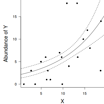
Finally, we will create a summary plot.
par(mar = c(4, 5, 0, 0))
plot(y ~ x, data = dat.qp, type = "n", ann = F, axes = F)
points(y ~ x, data = dat.qp, pch = 16)
xs <- seq(0, 20, l = 1000)
coefs <- fixef(dat.qp.glmm)
mm <- model.matrix(~x, data=data.frame(x=xs))
ys <- as.vector(coefs %*% t(mm))
se <- sqrt(diag(mm %*% vcov(dat.qp.glmm) %*% t(mm)))
lwr <- exp(ys-qt(0.975,dat.qp.glmm$fixDF$X[2])*se)
upr <- exp(ys+qt(0.975,dat.qp.glmm$fixDF$X[2])*se)
lwr50 <- exp(ys-se)
upr50 <- exp(ys+se)

points(exp(ys) ~ xs, col = "black", type = "l")
#lines(lwr ~ xs, col = "black", type = "l", lty = 2)
#lines(upr ~ xs, col = "black", type = "l", lty = 2)
lines(lwr50 ~ xs, col = "black", type = "l", lty = 2)
lines(upr50 ~ xs, col = "black", type = "l", lty = 2)
axis(1)
mtext("X", 1, cex = 1.5, line = 3)
axis(2, las = 2)
mtext("Abundance of Y", 2, cex = 1.5, line = 3)
box(bty = "l")
Negative binomial regression
Scenario and Data
Lets say we wanted to model the abundance of an item ($y$) against a continuous predictor ($x$). As this section is mainly about the generation of artificial data (and not specifically about what to do with the data), understanding the actual details are optional and can be safely skipped. Consequently, I have folded (toggled) this section away.
Random data incorporating the following trends (effect parameters)- the sample size = 20
- the continuous $x$ variable is a random uniform spread of measurements between 1 and 20
- the rate of change in log $y$ per unit of $x$ (slope) = 0.1.
- the value of $x$ when log$y$ equals 0 (when $y$=1)
- to generate the values of $y$ expected at each $x$ value, we evaluate the linear predictor (created by calculating the outer product of the model matrix and the regression parameters). These expected values are then transformed into a scale mapped by (0,$\infty$) by using the log function $e^{linear~predictor}$
- finally, we generate $y$ values by using the expected $y$ values ($\lambda$) as probabilities when drawing random numbers from a Poisson distribution. This step adds random noise to the expected $y$ values and returns only 0's and positive integers.
set.seed(37) #16 #35
#The number of samples
n.x <- 20
#Create x values that at uniformly distributed throughout the rate of 1 to 20
x <- sort(runif(n = n.x, min = 1, max =20))
mm <- model.matrix(~x)
intercept <- 0.6
slope=0.1
#The linear predictor
linpred <- mm %*% c(intercept,slope)
#Predicted y values
lambda <- exp(linpred)
#Add some noise and make binomial
y <- rnbinom(n=n.x, mu=lambda, size=1)
dat.nb <- data.frame(y,x)
data.nb <- dat.nb
write.table(data.nb, file='../downloads/data/data.nb.csv', quote=F, row.names=F, sep=',')
Exploratory data analysis and initial assumption checking
The assumptions are:- All of the observations are independent - this must be addressed at the design and collection stages
- The response variable (and thus the residuals) should be matched by an appropriate distribution (in the case of positive integers response - a Poisson is appropriate).
- All observations are equally influential in determining the trends - or at least no observations are overly influential. This is most effectively diagnosed via residuals and other influence indices and is very difficult to diagnose prior to analysis
- the relationship between the linear predictor (right hand side of the regression formula) and the link function should be linear. A scatterplot with smoother can be useful for identifying possible non-linearity.
- Dispersion is either 1 or overdispersion is otherwise accounted for in the model
- The number of zeros is either not excessive or else they are specifically addressed by the model
When counts are all very large (not close to 0) and their ranges do not span orders of magnitude, they take on very Gaussian properties (symmetrical distribution and variance independent of the mean). Given that models based on the Gaussian distribution are more optimized and recognized than Generalized Linear Models, it can be prudent to adopt Gaussian models for such data. Hence it is a good idea to first explore whether a Poisson model is likely to be more appropriate than a standard Gaussian model.
Recall from Poisson regression, there are five main potential models that we could consider fitting to these data.
There are five main potential models we could consider fitting to these data:
- Ordinary least squares regression (general linear model) - assumes normality of residuals
- Poisson regression - assumes mean=variance (dispersion=1)
- Quasi-poisson regression - a general solution to overdispersion. Assumes variance is a function of mean, dispersion estimated, however likelihood based statistics unavailable
- Negative binomial regression - a specific solution to overdispersion caused by clumping (due to an unmeasured latent variable). Scaling factor ($\omega$) is estimated along with the regression parameters.
- Zero-inflation model - a specific solution to overdispersion caused by excessive zeros (due to an unmeasured latent variable). Mixture of binomial and Poisson models.
Confirm non-normality and explore clumping
Check the distribution of the $y$ abundances
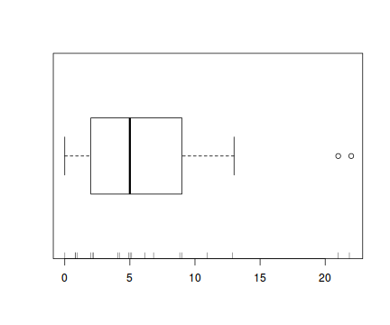
There is definitely signs of non-normality that would warrant Poisson models. Further to that, the rug on the boxplot is suggestive of clumping (observations are not evenly distributed and well spaced out). Together the, skewness and clumping could point to an overdispersed Poisson. Negative binomial models are the most effective at modeling such data.hist(dat.nb$y)
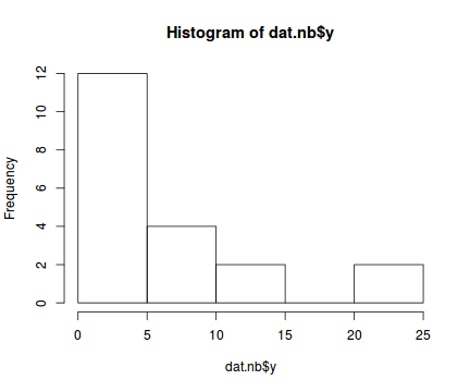
boxplot(dat.nb$y, horizontal=TRUE)
rug(jitter(dat.nb$y))
Confirm linearity
Lets now explore linearity by creating a histogram of the predictor variable ($x$) and a scatterplot of the relationship between the response ($y$) and the predictor ($x$)
hist(dat.nb$x)

#now for the scatterplot
plot(y~x, dat.nb, log="y")
with(dat.nb, lines(lowess(y~x)))
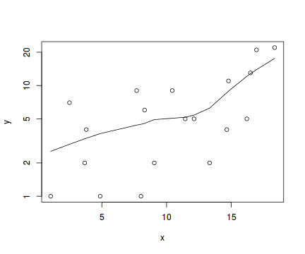
Conclusions: the predictor ($x$) does not display any skewness or other issues that might lead to non-linearity. The lowess smoother on the scatterplot does not display major deviations from a straight line and thus linearity is satisfied. Violations of linearity could be addressed by either:
- define a non-linear linear predictor (such as a polynomial, spline or other non-linear function)
- transform the scale of the predictor variables
Explore the distributional properties of the response
Lets explore the goodness of fit of the data to both Poisson and Negative Binomial distributions.
library(vcd)
fit <- goodfit(dat.nb$y, type='poisson')
summary(fit)
Goodness-of-fit test for poisson distribution X^2 df P(> X^2) Likelihood Ratio 73.64611 10 8.722665e-12rootogram(fit)
fit <- goodfit(dat.nb$y, type='nbinom')
summary(fit)
Goodness-of-fit test for nbinomial distribution X^2 df P(> X^2) Likelihood Ratio 22.38866 9 0.007725515rootogram(fit)
Ord_plot(dat.nb$y, tol=0.2)
distplot(dat.nb$y, type='poisson')
distplot(dat.nb$y, type="nbinom")
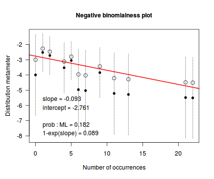
Conclusions - not withstanding the very small sample sizes, it would appear that a Negative Binomial is a better fit to the data than a Poisson. Note, the Ord plot is likely to be suffering due to the small sample size and I am going to ignore it.
Explore zero inflation
Although we have already established that there are few zeros in the data (and thus overdispersion is unlikely to be an issue), we can also explore this by comparing the number of zeros in the data to the number of zeros that would be expected from a Poisson distribution with a mean equal to the mean count of the data.
In the above, the value under FALSE is the proportion of non-zero values in the data and the value under TRUE is the proportion of zeros in the data. In this example, the proportion of zeros observed is similar to the proportion expected. Indeed, there was only a single zero observed. Hence it is likely that if there is overdispersion it is unlikely to be due to excessive zeros.#proportion of 0's in the data dat.nb.tab<-table(dat.nb$y==0) dat.nb.tab/sum(dat.nb.tab)
FALSE  TRUE
 0.95  0.05
#proportion of 0's expected from a Poisson distribution
mu <- mean(dat.nb$y)
cnts <- rpois(1000, mu)
dat.nb.tabE <- table(cnts == 0)
dat.nb.tabE/sum(dat.nb.tabE)
FALSE 1Model fitting or statistical analysis
The boxplot of $y$ with the axis rug suggested that there might be some clumping (possibly due to some other unmeasured influence). We will therefore perform negative binomial regression using the glm.nb() function. The most important (=commonly used) parameters/arguments for negative binomial regression are:
- formula: the linear model relating the response variable to the linear predictor
- data: the data frame containing the data
I will now fit the negative binomial regression: $$log(\mu)=\beta_0+\beta_1x_1+\epsilon_i, \hspace{1cm}\epsilon\sim NB(\lambda, \phi)$$
library(MASS)
dat.nb.glm <- glm.nb(y~x, data=dat.nb)
Model evaluation
Prior to exploring the model parameters, it is prudent to confirm that the model did indeed fit the assumptions and was an appropriate fit to the data. There are a number of extractor functions (functions that extract or derive specific information from a model) available including:
Extractor Description residuals() Extracts the residuals from the model fitted() Extracts the predicted (expected) response values (on the link scale) at the observed levels of the linear predictor predict() Extracts the predicted (expected) response values (on either the link, response or terms (linear predictor) scale) coef() Extracts the model coefficients deviance() Extracts the deviance from the model AIC() Extracts the Akaike's Information Criterion from the model extractAIC() Extracts the generalized Akaike's Information Criterion from the model summary() Summarizes the important output and characteristics of the model anova() Computes an analysis of deviance or log-likelihood ratio test (LRT) from the model plot() Generates a series of diagnostic plots from the model Lets explore the diagnostics - particularly the residuals
And now exploring the simulated residuals via the DHARMa package.plot(dat.nb.glm)
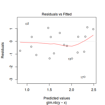
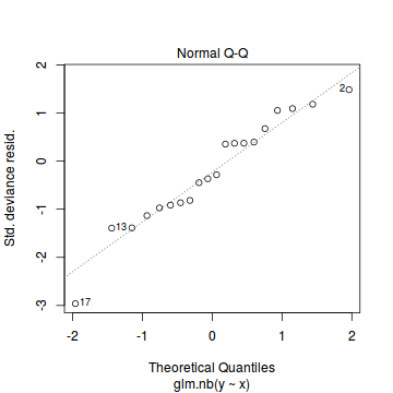
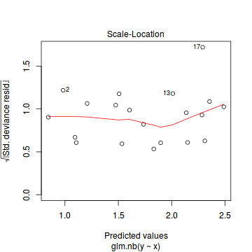
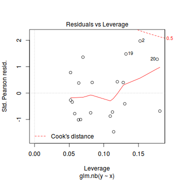 Conclusions: there is no obvious patterns in the residuals, or at least there are no obvious trends remaining that would be indicative of non-linearity.
library(DHARMa)
dat.nb.sim <- simulateResiduals(dat.nb.glm)
dat.nb.sim
[1] "Class DHARMa with simulated residuals based on 250 simulations with refit = FALSE"
[1] "see ?DHARMa::simulateResiduals for help"
[1] "-----------------------------"
 [1] 0.416 0.964 0.504 0.724 0.276 0.940 0.208 0.748 0.300 0.804 0.460 0.504 0.204 0.296 0.720 0.328
[17] 0.028 0.712 0.892 0.896
plotSimulatedResiduals(dat.nb.sim)
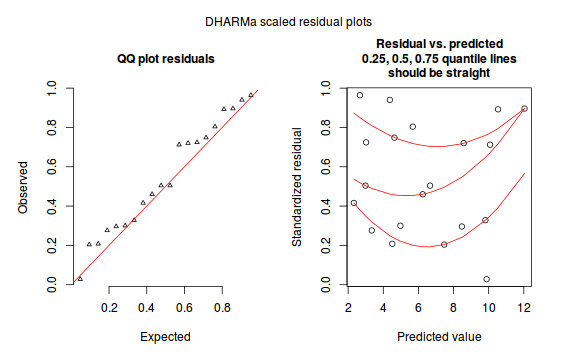
Exploring goodness-of-fit, overdispersion and zero-inflation
The negative binomial family should handle the majority of overdispersion. However, zero-inflation can still be an issue.
- Kolmogorov-Smirnov test for uniformity
testUniformity(dat.nb.sim)
	One-sample Kolmogorov-Smirnov test

data:  simulationOutput$scaledResiduals
D = 0.162, p-value = 0.6702
alternative hypothesis: two-sided
- Exploring overdispersion
dat.nb.sim <- simulateResiduals(dat.nb.glm, refit=T)
testOverdispersion(dat.nb.sim)
	Overdispersion test via comparison to simulation under H0

data:  dat.nb.sim
dispersion = 0.83369, p-value = 0.892
alternative hypothesis: overdispersion
- Exploring zero-inflation
testZeroInflation(dat.nb.sim)
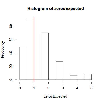
	Zero-inflation test via comparison to expected zeros with simulation under H0

data:  dat.nb.sim
ratioObsExp = 0.66667, p-value = 0.444
alternative hypothesis: more
Comparing fitted values to observed counts
tempdata <- data.frame(obs=dat.nb$y, fitted=fitted(dat.nb.glm))
library(ggplot2)
ggplot(tempdata, aes(y=fitted, x=obs)) + geom_point()
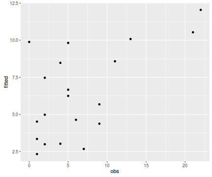
Conclusions - the relationship between fitted values and observed counts is reasonable without being spectacular.
In this demonstration we fitted the Negative binomial model. As well as estimating the regression coefficients, the negative binomial also estimates the dispersion parameter ($\phi$), thus requiring an additional degree of freedom. We could compare the fit of the negative binomial to that of a regular Poisson model (that assumes a dispersion of 1), using AIC.
Conclusions: The AIC is smaller for the Negative binomial model, suggesting that it is a better fit than the Poisson model.dat.glm <- glm(y~x, data=dat.nb, family="poisson") AIC(dat.nb.glm, dat.glm)
Error in AIC.glm(dat.nb.glm, dat.glm): unused argument (dat.glm)
Exploring the model parameters, test hypotheses
If there was any evidence that the assumptions had been violated or the model was not an appropriate fit, then we would need to reconsider the model and start the process again. In this case, there is no evidence that the test will be unreliable so we can proceed to explore the test statistics. The main statistic of interest is the Wald statistic ($z$) for the slope parameter.
summary(dat.nb.glm)
Call:
glm.nb(formula = y ~ x, data = dat.nb, init.theta = 2.359878187,
    link = log)

Deviance Residuals:
    Min       1Q   Median       3Q      Max
-2.7874  -0.8940  -0.3172   0.4420   1.3660

Coefficients:
            Estimate Std. Error z value Pr(>|z|)
(Intercept)  0.74543    0.42534   1.753  0.07968 .
x            0.09494    0.03441   2.759  0.00579 **
---
Signif. codes:  0 '***' 0.001 '**' 0.01 '*' 0.05 '.' 0.1 ' ' 1

(Dispersion parameter for Negative Binomial(2.3599) family taken to be 1)

    Null deviance: 30.443  on 19  degrees of freedom
Residual deviance: 21.806  on 18  degrees of freedom
AIC: 115.85

Number of Fisher Scoring iterations: 1


              Theta:  2.36
          Std. Err.:  1.10

 2 x log-likelihood:  -109.849
Conclusions: We would reject the null hypothesis (p<0.05). An increase in x is associated with a significant linear increase (positive slope) in log $y$ abundance. Every 1 unit increase in $x$ is associated with a 0.1115 unit increase in $\log y$ abundance We usually express this in terms of $y$ than $\log y$, so every 1 unit increase in $x$ is associated with a ($e^{0.1115}=1.12$) 1.12 unit increase in $y$ abundance.
P-values are widely acknowledged as a rather flawed means of inference testing (as in hypothesis testing in general). An alternate way of exploring the characteristics of parameter estimates is to calculate their confidence intervals. Confidence intervals that do not overlap with the null hypothesis parameter value (e.g. effect of 0), are an indication of a significant effect. Recall however, that in frequentist statistics the confidence intervals are interpreted as the range of values that are likely to contain the true mean on 95 out of 100 (95%) repeated samples.
Conclusions: A 1 unit increase in $x$ is associated with a ($e^{0.62}=1.89$) 1.89 (1.14,3.02) unit increase in $y$ abundance.library(gmodels) ci(dat.nb.glm)
              Estimate    CI lower CI upper Std. Error     p-value
(Intercept) 0.74542589 -0.14818316 1.639035 0.42534137 0.079681751
x           0.09493852  0.02265303 0.167224 0.03440655 0.005792266
Further explorations of the trends
A measure of the strength of the relationship can be obtained according to: $$quasi R^2 = 1-\left(\frac{deviance}{null~deviance}\right)$$
Conclusions: approximately1-(dat.nb.glm$deviance/dat.nb.glm$null)
[1] 0.2836978
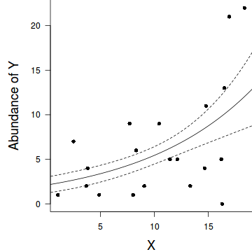
28.4% of the variability in abundance can be explained by its relationship to $x$. Technically, it is28.4% of the variability in $\log y$ (the link function) is explained by its relationship to $x$.Finally, we will create a summary plot.
par(mar = c(4, 5, 0, 0))
plot(y ~ x, data = dat.nb, type = "n", ann = F, axes = F)
points(y ~ x, data = dat.nb, pch = 16)
xs <- seq(0, 20, l = 1000)
ys <- predict(dat.nb.glm, newdata = data.frame(x = xs), type = "response", se = T)
points(ys$fit ~ xs, col = "black", type = "l")
lines(ys$fit - 1 * ys$se.fit ~ xs, col = "black", type = "l", lty = 2)
lines(ys$fit + 1 * ys$se.fit ~ xs, col = "black", type = "l", lty = 2)
axis(1)
mtext("X", 1, cex = 1.5, line = 3)
axis(2, las = 2)
mtext("Abundance of Y", 2, cex = 1.5, line = 3)
box(bty = "l")
Zero-inflation Poisson (ZIP) regression
Scenario and Data
Lets say we wanted to model the abundance of an item ($y$) against a continuous predictor ($x$). As this section is mainly about the generation of artificial data (and not specifically about what to do with the data), understanding the actual details are optional and can be safely skipped. Consequently, I have folded (toggled) this section away.
Random data incorporating the following trends (effect parameters)- the sample size = 20
- the continuous $x$ variable is a random uniform spread of measurements between 1 and 20
- the rate of change in log $y$ per unit of $x$ (slope) = 0.1.
- the value of $x$ when log$y$ equals 0 (when $y$=1)
- to generate the values of $y$ expected at each $x$ value, we evaluate the linear predictor (created by calculating the outer product of the model matrix and the regression parameters). These expected values are then transformed into a scale mapped by (0,$\infty$) by using the log function $e^{linear~predictor}$
- finally, we generate $y$ values by using the expected $y$ values ($\lambda$) as probabilities when drawing random numbers from a Poisson distribution. This step adds random noise to the expected $y$ values and returns only 0's and positive integers.
set.seed(37) #34.5  #4 #10 #16 #17 #26
#The number of samples
n.x <- 20
#Create x values that at uniformly distributed throughout the rate of 1 to 20
x <- sort(runif(n = n.x, min = 1, max =20))
mm <- model.matrix(~x)
intercept <- 0.6
slope=0.1
#The linear predictor
linpred <- mm %*% c(intercept,slope)
#Predicted y values
lambda <- exp(linpred)
#Add some noise and make binomial
library(gamlss.dist)
#fixed latent binomial
y<- rZIP(n.x,lambda, 0.4)
#latent binomial influenced by the linear predictor
#y<- rZIP(n.x,lambda, 1-exp(linpred)/(1+exp(linpred)))
dat.zip <- data.frame(y,x)

data.zip <- dat.zip
write.table(data.zip, file='../downloads/data/data.zip.csv', quote=F, row.names=F, sep=',')

summary(glm(y~x, dat.zip, family="poisson"))
Call: glm(formula = y ~ x, family = "poisson", data = dat.zip) Deviance Residuals: Min 1Q Median 3Q Max -2.5415 -2.3769 -0.9753 1.1736 3.6380 Coefficients: Estimate Std. Error z value Pr(>|z|) (Intercept) 0.67048 0.33018 2.031 0.0423 * x 0.02961 0.02663 1.112 0.2662 --- Signif. codes: 0 '***' 0.001 '**' 0.01 '*' 0.05 '.' 0.1 ' ' 1 (Dispersion parameter for poisson family taken to be 1) Null deviance: 85.469 on 19 degrees of freedom Residual deviance: 84.209 on 18 degrees of freedom AIC: 124.01 Number of Fisher Scoring iterations: 6plot(glm(y~x, dat.zip, family="poisson"))
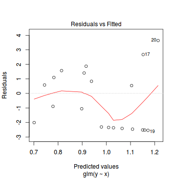
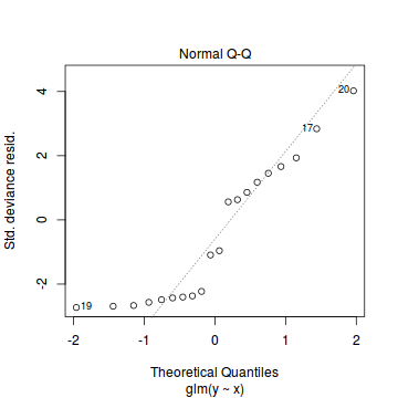
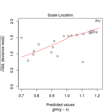
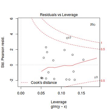
library(pscl)
summary(zeroinfl(y ~ x | 1, dist = "poisson", data = dat.zip))
Call: zeroinfl(formula = y ~ x | 1, data = dat.zip, dist = "poisson") Pearson residuals: Min 1Q Median 3Q Max -1.0015 -0.9556 -0.3932 0.9663 1.6195 Count model coefficients (poisson with log link): Estimate Std. Error z value Pr(>|z|) (Intercept) 0.70474 0.31960 2.205 0.027449 * x 0.08734 0.02532 3.449 0.000563 *** Zero-inflation model coefficients (binomial with logit link): Estimate Std. Error z value Pr(>|z|) (Intercept) -0.2292 0.4563 -0.502 0.615 --- Signif. codes: 0 '***' 0.001 '**' 0.01 '*' 0.05 '.' 0.1 ' ' 1 Number of iterations in BFGS optimization: 13 Log-likelihood: -36.17 on 3 Dfplot(resid(zeroinfl(y ~ x | 1, dist = "poisson", data = dat.zip))~fitted(zeroinfl(y ~ x | 1, dist = "poisson", data = dat.zip)))
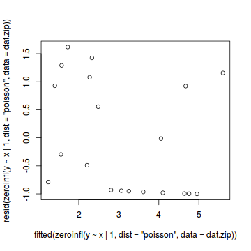
library(gamlss)
summary(gamlss(y~x,data=dat.zip, family=ZIP))
GAMLSS-RS iteration 1: Global Deviance = 72.4363 GAMLSS-RS iteration 2: Global Deviance = 72.3428 GAMLSS-RS iteration 3: Global Deviance = 72.3428 ******************************************************************* Family: c("ZIP", "Poisson Zero Inflated") Call: gamlss(formula = y ~ x, family = ZIP, data = dat.zip) Fitting method: RS() ------------------------------------------------------------------- Mu link function: log Mu Coefficients: Estimate Std. Error t value Pr(>|t|) (Intercept) 0.70582 0.31958 2.209 0.04123 * x 0.08719 0.02533 3.442 0.00311 ** --- Signif. codes: 0 '***' 0.001 '**' 0.01 '*' 0.05 '.' 0.1 ' ' 1 ------------------------------------------------------------------- Sigma link function: logit Sigma Coefficients: Estimate Std. Error t value Pr(>|t|) (Intercept) -0.2292 0.4563 -0.502 0.622 ------------------------------------------------------------------- No. of observations in the fit: 20 Degrees of Freedom for the fit: 3 Residual Deg. of Freedom: 17 at cycle: 3 Global Deviance: 72.34282 AIC: 78.34282 SBC: 81.33002 *******************************************************************predict(gamlss(y~x,data=dat.zip, family=ZIP), se.fit=TRUE, what="mu")
GAMLSS-RS iteration 1: Global Deviance = 72.4363
GAMLSS-RS iteration 2: Global Deviance = 72.3428
GAMLSS-RS iteration 3: Global Deviance = 72.3428
$fit
        1         2         3         4         5         6         7         8         9        10
0.7966905 0.9236189 1.0263933 1.0369823 1.1305358 1.3763304 1.4054417 1.4299603 1.4951229 1.6161339
       11        12        13        14        15        16        17        18        19        20
1.7035853 1.7629994 1.8678543 1.9838052 1.9951833 2.1187071 2.1249555 2.1431616 2.1837285 2.3064727

$se.fit
        1         2         3         4         5         6         7         8         9        10
0.3517894 0.3089432 0.2758980 0.2726011 0.2445792 0.1856062 0.1807322 0.1770893 0.1696661 0.1656458
       11        12        13        14        15        16        17        18        19        20
0.1710016 0.1783138 0.1973009 0.2251987 0.2282363 0.2637860 0.2656903 0.2712879 0.2840032 0.3241532
Exploratory data analysis and initial assumption checking
The assumptions are:- All of the observations are independent - this must be addressed at the design and collection stages
- The response variable (and thus the residuals) should be matched by an appropriate distribution (in the case of positive integers response - a Poisson is appropriate).
- All observations are equally influential in determining the trends - or at least no observations are overly influential. This is most effectively diagnosed via residuals and other influence indices and is very difficult to diagnose prior to analysis
- the relationship between the linear predictor (right hand side of the regression formula) and the link function should be linear. A scatterplot with smoother can be useful for identifying possible non-linearity.
- Dispersion is either 1 or overdispersion is otherwise accounted for in the model
- The number of zeros is either not excessive or else they are specifically addressed by the model
Confirm non-normality and explore clumping
Check the distribution of the $y$ abundances
There is definitely signs of non-normality that would warrant Poisson models. Further to that, there appears to be a large number of zeros that are likely to be the cause of overdispersion A zero-inflated Poisson model is likely to be one of the most effective for modeling these data.hist(dat.zip$y)
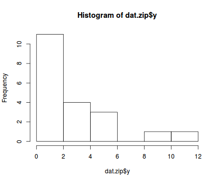
boxplot(dat.zip$y, horizontal=TRUE)
rug(jitter(dat.zip$y))
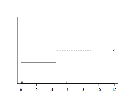
Confirm linearity
Lets now explore linearity by creating a histogram of the predictor variable ($x$). Note, it is difficult to directly assess issues of linearity. Indeed, a scatterplot with lowess smoother will be largely influenced by the presence of zeros. One possible way of doing so is to explore the trend in the non-zero data.
hist(dat.zip$x)
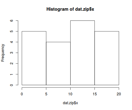
#now for the scatterplot
plot(y~x, dat.zip, log="y")
with(subset(dat.zip,y>0), lines(lowess(y~x)))
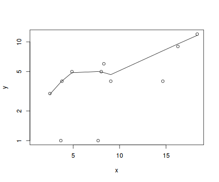
Conclusions: the predictor ($x$) does not display any skewness or other issues that might lead to non-linearity. The lowess smoother on the non-zero data cloud does not display major deviations from a straight line and thus linearity is likely to be satisfied. Violations of linearity (whilst difficult to be certain about due to the unknown influence of the zeros) could be addressed by either:
- define a non-linear linear predictor (such as a polynomial, spline or other non-linear function)
- transform the scale of the predictor variables
Explore zero inflation
Although we have already established that there are few zeros in the data (and thus overdispersion is unlikely to be an issue), we can also explore this by comparing the number of zeros in the data to the number of zeros that would be expected from a Poisson distribution with a mean equal to the mean count of the data.
In the above, the value under FALSE is the proportion of non-zero values in the data and the value under TRUE is the proportion of zeros in the data. In this example, the proportion of zeros observed (45%) far exceeds that that would have been expected (8%). Hence it is highly likely that any models will be zero-inflated.#proportion of 0's in the data dat.zip.tab<-table(dat.zip$y==0) dat.zip.tab/sum(dat.zip.tab)
FALSE  TRUE
 0.55  0.45
#proportion of 0's expected from a Poisson distribution
mu <- mean(dat.zip$y)
cnts <- rpois(1000, mu)
dat.zip.tabE <- table(cnts == 0)
dat.zip.tabE/sum(dat.zip.tabE)
FALSE  TRUE
0.921 0.079
Explore the distributional properties of the response
Lets explore the goodness of fit of the data to both Poisson and Negative Binomial distributions.
library(vcd)
fit <- goodfit(dat.zip$y, type='poisson')
summary(fit)
Goodness-of-fit test for poisson distribution X^2 df P(> X^2) Likelihood Ratio 53.12481 6 1.107313e-09rootogram(fit)
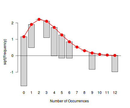
fit <- goodfit(dat.zip$y, type='nbinom')
summary(fit)
Goodness-of-fit test for nbinomial distribution X^2 df P(> X^2) Likelihood Ratio 15.80482 5 0.007424002rootogram(fit)
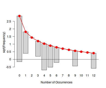
Ord_plot(dat.zip$y, tol=0.2)
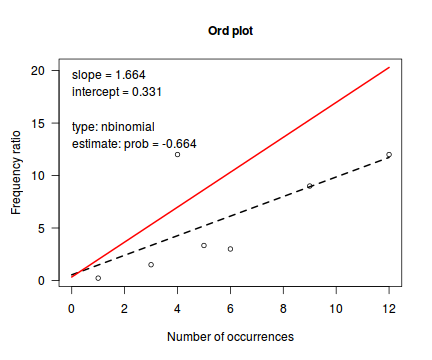
distplot(dat.zip$y, type='poisson')
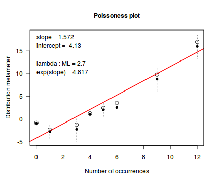
distplot(dat.zip$y, type="nbinom")
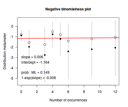
Conclusions - again not withstanding the very small sample sizes, it would appear that a Negative Binomial is a better fit to the data than a Poisson. That said, we have already established that the data are likely to be zero inflated and thus some of the reason that the Negative Binomial might be favoured over the Poisson is that zero-inflated data are overdispersed. Perhaps if we tackle zero-inflation directly, the data wont be overdispersed.
Model fitting or statistical analysis
The exploratory data analyses have suggested that a zero-inflated Poisson model might be the most appropriate for these data. Zero-inflated models can be fit via functions from one of two packages within R:
- zeroinf() from the pscl package.
The most important (=commonly used) parameters/arguments for this function are:
- formula: the linear model relating the response variable to the linear predictor
- data: the data frame containing the data
- dist: a character specification of the distribution used to model the count data ("poisson", "negbin" or "geometric").
- gamlss() from the gamlss package.
This function (and more generally, the package) fits generalized additive models
(GAM) in a manner similar to the gam function in the gam package yet also accommodates a far
wider range of distributions (including non-exponentials). All distribution parameters can be modeled against the linear predictor
The most important (=commonly used) parameters/arguments for this function are:
- formula: the linear model relating the response variable to the linear predictor
- data: the data frame containing the data
- family: an object defining the distribution(s) (and link functions) for the various parameters.
I will now fit the Zero-Inflation Poisson (ZIP) regression via both functions: $$ y = \begin{cases} 0 ~ \text{with} ~Pr(y_i) = 1-\mu, & logit(\omega)=\alpha_0+\delta(\mu)+\epsilon_i, \hspace{1cm}&\epsilon\sim Binom(\pi)\\ >0 & log(\mu)=\beta_0+\beta_1x_1+\epsilon_i, &\epsilon\sim Poisson(\mu)\\ \end{cases} $$
- zeroinfl
The formula in the above indicates that the Poisson component is modeled against the linear predictor that includes the predictor variable ($x$) whereas the binomial component is modeled against a constant.
library(pscl)
dat.zeroinfl <- zeroinfl(y~x|1, data=dat.zip, dist="poisson")
- gamlss
library(gamlss)
dat.gamlss <- gamlss(y~x, data=dat.zip, family=ZIP)
GAMLSS-RS iteration 1: Global Deviance = 72.4363
GAMLSS-RS iteration 2: Global Deviance = 72.3428
GAMLSS-RS iteration 3: Global Deviance = 72.3428
Model evaluation
Prior to exploring the model parameters, it is prudent to confirm that the model did indeed fit the assumptions and was an appropriate fit to the data.
Lets explore the diagnostics - particularly the residuals
- zeroinfl
There are a number of extractor functions (functions that extract or derive specific information from a model) available including:
Extractor Description residuals() Extracts the residuals from the model fitted() Extracts the predicted (expected) response values (on the link scale) at the observed levels of the linear predictor predict() Extracts the predicted (expected) response values (on either the model="response", model="prob", model="count" or model="zero" link scale) coef() Extracts the model coefficients for either the Poisson (model="count") or binomial (model="zero") components vcov() Extracts the variance-covariance matrix for either the Poisson (model="count") or binomial (model="zero") components summary() Summarizes the important output and characteristics of the model terms() Extracts the terms for either the Poisson (model="count") or binomial (model="zero") components model.matrix() Extracts the model matrix for either the Poisson (model="count") or binomial (model="zero") components plot(resid(dat.zeroinfl)~fitted(dat.zeroinfl))
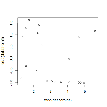
- gamlss
There are a number of extractor functions (functions that extract or derive specific information from a model) available including:
Extractor Description residuals() Extracts the residuals from the model. Residuals can either be standardized (what="z-scores") or be for specific parameters (model="mu", model="sigma", model="nu" or model="tau"). fitted() Extracts the predicted (expected) response values (on the link scale) at the observed levels of the linear predictor. Fitted values are for one of the specific parameters (what="mu", what="sigma", what="nu" or what="tau"). predict() Extracts the predicted (expected) response values (on either the type="link", type="response" or type="terms" (linear predictor ) scale). Predicted values are for one of the specific parameters (what="mu", what="sigma", what="nu" or what="tau"). coef() Extracts the model coefficients for one of the specific parameters (what="mu", what="sigma", what="nu" or what="tau"). vcov() Extracts the matrix of either variance-covariances (type="vcov"), correlations (type="cor"), standard errors (type="se"), coefficients (type="coef") or all (type="all") AIC() Extracts the Akaike's Information Criterion from the model extractAIC() Extracts the generalized Akaike's Information Criterion from the model summary() Summarizes the important output and characteristics of the model terms() Extracts the terms for one of the specific parameters (what="mu", what="sigma", what="nu" or what="tau"). model.matrix() Extracts the model matrix for one of the specific parameters (what="mu", what="sigma", what="nu" or what="tau"). plot(dat.gamlss)
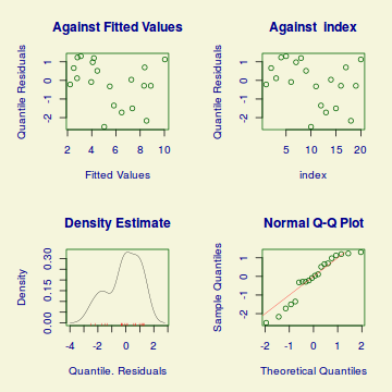
*******************************************************************
	 Summary of the Randomised Quantile Residuals
                           mean   =  -0.1288796
                       variance   =  1.369514
               coef. of skewness  =  -0.5522303
               coef. of kurtosis  =  2.0374
Filliben correlation coefficient  =  0.9623945
*******************************************************************
In this demonstration we fitted two ZIP models. We could compare the fit of each of these zero-inflated poisson models to that of a regular Poisson model (that assumes a dispersion of 1 and no excessive zeros), using AIC.
Conclusions: The AIC is substantially smaller for the zero-inflated poisson models than the standard Poisson regression model. Hence we would conclude that the zero-inflated models are a better fit than the Poisson regression model.dat.glm <- glm(y~x, data=dat.zip, family="poisson") AIC(dat.zeroinfl, dat.gamlss, dat.glm)
             df       AIC
dat.zeroinfl  3  78.34277
dat.gamlss    3  78.34282
dat.glm       2 124.00663
Comparing fitted values to observed counts
- zeroinf
tempdata <- data.frame(obs=dat.zip$y, fitted=fitted(dat.zeroinfl))
library(ggplot2)
ggplot(tempdata, aes(y=fitted, x=obs)) + geom_point()
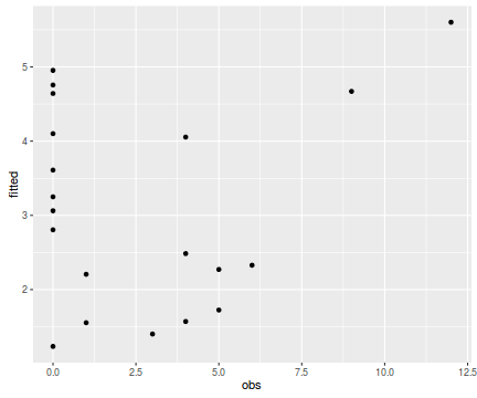
- gamlss
tempdata <- data.frame(obs=dat.zip$y, fitted=fitted(dat.gamlss))
library(ggplot2)
ggplot(tempdata, aes(y=fitted, x=obs)) + geom_point()
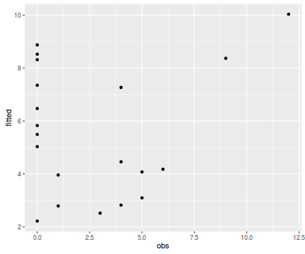
- zeroinfl
summary(dat.zeroinfl)
Call: zeroinfl(formula = y ~ x | 1, data = dat.zip, dist = "poisson") Pearson residuals: Min 1Q Median 3Q Max -1.0015 -0.9556 -0.3932 0.9663 1.6195 Count model coefficients (poisson with log link): Estimate Std. Error z value Pr(>|z|) (Intercept) 0.70474 0.31960 2.205 0.027449 * x 0.08734 0.02532 3.449 0.000563 *** Zero-inflation model coefficients (binomial with logit link): Estimate Std. Error z value Pr(>|z|) (Intercept) -0.2292 0.4563 -0.502 0.615 --- Signif. codes: 0 '***' 0.001 '**' 0.01 '*' 0.05 '.' 0.1 ' ' 1 Number of iterations in BFGS optimization: 13 Log-likelihood: -36.17 on 3 Df - gamlss
summary(dat.gamlss)
******************************************************************* Family: c("ZIP", "Poisson Zero Inflated") Call: gamlss(formula = y ~ x, family = ZIP, data = dat.zip) Fitting method: RS() ------------------------------------------------------------------- Mu link function: log Mu Coefficients: Estimate Std. Error t value Pr(>|t|) (Intercept) 0.70582 0.31958 2.209 0.04123 * x 0.08719 0.02533 3.442 0.00311 ** --- Signif. codes: 0 '***' 0.001 '**' 0.01 '*' 0.05 '.' 0.1 ' ' 1 ------------------------------------------------------------------- Sigma link function: logit Sigma Coefficients: Estimate Std. Error t value Pr(>|t|) (Intercept) -0.2292 0.4563 -0.502 0.622 ------------------------------------------------------------------- No. of observations in the fit: 20 Degrees of Freedom for the fit: 3 Residual Deg. of Freedom: 17 at cycle: 3 Global Deviance: 72.34282 AIC: 78.34282 SBC: 81.33002 ******************************************************************* - Logan (2010) - Chpt 16-17
- Quinn & Keough (2002) - Chpt 13-14
-
Is there any evidence that these assumptions have been violated?
Show codeboxplot(Count~Shore, data=limpets)
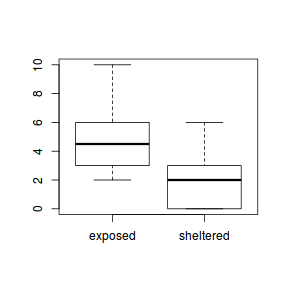
library(vcd) fit <- goodfit(limpets$Count, type='poisson') summary(fit)
Goodness-of-fit test for poisson distribution X^2 df P(> X^2) Likelihood Ratio 14.03661 7 0.05053407rootogram(fit)
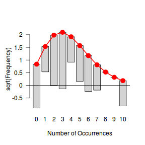
fit <- goodfit(limpets$Count, type='nbinom') summary(fit)
Goodness-of-fit test for nbinomial distribution X^2 df P(> X^2) Likelihood Ratio 9.105475 6 0.1677325rootogram(fit)
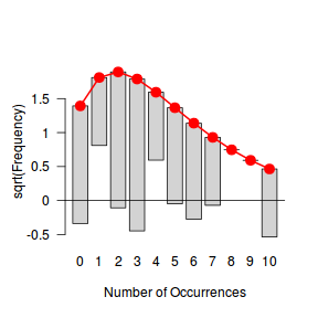
Ord_plot(limpets$Count, tol=0.2)
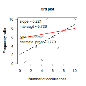
distplot(limpets$Count, type='poisson')
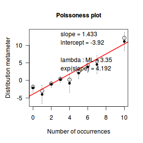
## Although we could argue that NB more appropriate than Poisson, this is possibly ## due to the small sample size. Small samples are more varied than the populations ## from which they are drawn
- The assumption of normality has been violated?
- The assumption of homogeneity of variance has been violated?
- Notwithstanding the very small sample size, is a Poisson distribution appropriate?
- The assumption of normality has been violated?
- Lets instead we fit the same model with a Poisson distribution.
$$log(\mu) = \beta_0+\beta1Shore_i+\epsilon_i, \hspace{1cm} \epsilon \sim Poisson(\lambda)$$
Show code
limpets.glm <- glm(Count~Shore, family=poisson, data=limpets)
- Explore the patterns in simulated residuals:
Show code
library(DHARMa)
limpets.glm.sim <- simulateResiduals(limpets.glm) limpets.glm.sim
[1] "Class DHARMa with simulated residuals based on 250 simulations with refit = FALSE" [1] "see ?DHARMa::simulateResiduals for help" [1] "-----------------------------" [1] 0.620 0.656 0.044 0.988 0.120 0.880 0.732 0.032 0.216 0.720 0.632 0.208 0.644 0.312 0.496 0.820 [17] 0.952 0.268 0.484 0.048
plotSimulatedResiduals(limpets.glm.sim)
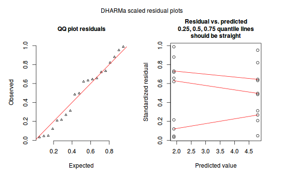
- Check the model for lack of fit via:
- Pearson Χ2
Show code
limpets.resid <- sum(resid(limpets.glm, type="pearson")^2) 1-pchisq(limpets.resid, limpets.glm$df.resid)
[1] 0.07874903
#No evidence of a lack of fit - Deviance (G2)
Show code
1-pchisq(limpets.glm$deviance, limpets.glm$df.resid)
[1] 0.05286849
#No evidence of a lack of fit - Standardized residuals (plot)
Show code
plot(limpets.glm)
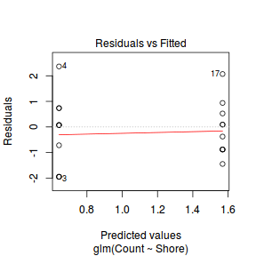
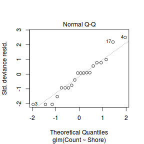
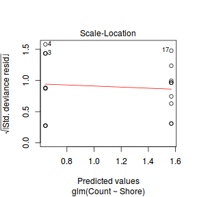
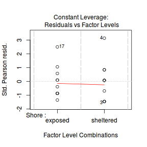
- Fitted and observed values (plot)
Show code
tempdata <- predict(limpets.glm, type='response', se=TRUE) tempdata <- cbind(limpets, Mean=tempdata[[1]], Lower=tempdata[[1]]-tempdata[[2]], Upper=tempdata[[1]]+tempdata[[2]]) library(ggplot2) ggplot(tempdata, aes(y=Count, x=Shore)) + geom_boxplot() + geom_pointrange(aes(y=Mean, ymin=Lower, ymax=Upper), color='red')
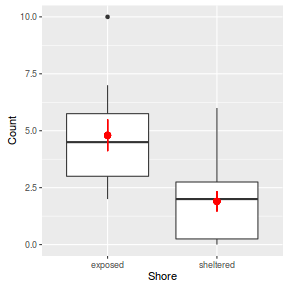
## the fitted values (red point range) are not inconsistent with the observed counts - Kolmogorov-Smirnov uniformity test
Show code
testUniformity(limpets.glm.sim)
One-sample Kolmogorov-Smirnov test data: simulationOutput$scaledResiduals D = 0.12, p-value = 0.9031 alternative hypothesis: two-sided
- Pearson Χ2
- Estimate the dispersion parameter to evaluate over dispersion in the fitted model
- Via Pearson residuals
Show code
limpets.resid/limpets.glm$df.resid
[1] 1.500731
#No evidence of over dispersion - Via deviance
Show code
limpets.glm$deviance/limpets.glm$df.resid
[1] 1.591496
#No evidence of over dispersion - Via $\alpha$
Show code
library(AER) dispersiontest(limpets.glm)
Overdispersion test data: limpets.glm z = 0.85688, p-value = 0.1958 alternative hypothesis: true dispersion is greater than 1 sample estimates: dispersion 1.350658
- Simulated residuals
Show code
limpets.glm.sim <- simulateResiduals(limpets.glm, refit=T) testOverdispersion(limpets.glm.sim)
Overdispersion test via comparison to simulation under H0 data: limpets.glm.sim dispersion = 1.506, p-value = 0.068 alternative hypothesis: overdispersion
## and overdispersion.. testZeroInflation(limpets.glm.sim)
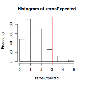
Zero-inflation test via comparison to expected zeros with simulation under H0 data: limpets.glm.sim ratioObsExp = 2.0161, p-value = 0.06 alternative hypothesis: more
- Via Pearson residuals
- Compare the expected number of zeros to the actual number of zeros to determine whether the model might be zero inflated.
- Calculate the proportion of zeros in the data
Show code
limpets.tab<-table(limpets$Count==0) limpets.tab/sum(limpets.tab)
FALSE TRUE 0.85 0.15
- Now work out the proportion of zeros we would expect from a Poisson distribution with a lambda equal to the mean count of limpets in this study.
Show codeThere are not substantially higher proportion of zeros than would be expected. The data a slightly zero inflated.
limpets.mu <- mean(limpets$Count) cnts <-rpois(1000,limpets.mu) limpets.tab<-table(cnts==0) limpets.tab/sum(limpets.tab)
FALSE TRUE 0.959 0.041
- Calculate the proportion of zeros in the data
- Explore the patterns in simulated residuals:
-
We can now test the null hypothesis that there is no effect of shore type on the abundance of striped limpets;
- Wald z-tests (these are equivalent to t-tests)
- Wald Chisq-test. Note that Chisq = z2
- Likelihood ratio test (LRT), analysis of deviance Chisq-tests (these are equivalent to ANOVA)
Show codesummary(limpets.glm)
Call: glm(formula = Count ~ Shore, family = poisson, data = limpets) Deviance Residuals: Min 1Q Median 3Q Max -1.94936 -0.88316 0.07192 0.57905 2.36619 Coefficients: Estimate Std. Error z value Pr(>|z|) (Intercept) 1.5686 0.1443 10.868 < 2e-16 *** Shoresheltered -0.9268 0.2710 -3.419 0.000628 *** --- Signif. codes: 0 '***' 0.001 '**' 0.01 '*' 0.05 '.' 0.1 ' ' 1 (Dispersion parameter for poisson family taken to be 1) Null deviance: 41.624 on 19 degrees of freedom Residual deviance: 28.647 on 18 degrees of freedom AIC: 85.567 Number of Fisher Scoring iterations: 5Show codelibrary(car) Anova(limpets.glm,test.statistic="Wald")
Analysis of Deviance Table (Type II tests) Response: Count Df Chisq Pr(>Chisq) Shore 1 11.691 0.000628 *** Residuals 18 --- Signif. codes: 0 '***' 0.001 '**' 0.01 '*' 0.05 '.' 0.1 ' ' 1Show codelimpets.glmN <- glm(Count~1, family=poisson, data=limpets) anova(limpets.glmN, limpets.glm, test="Chisq")
Analysis of Deviance Table Model 1: Count ~ 1 Model 2: Count ~ Shore Resid. Df Resid. Dev Df Deviance Pr(>Chi) 1 19 41.624 2 18 28.647 1 12.977 0.0003154 *** --- Signif. codes: 0 '***' 0.001 '**' 0.01 '*' 0.05 '.' 0.1 ' ' 1
# OR anova(limpets.glm, test="Chisq")
Analysis of Deviance Table Model: poisson, link: log Response: Count Terms added sequentially (first to last) Df Deviance Resid. Df Resid. Dev Pr(>Chi) NULL 19 41.624 Shore 1 12.977 18 28.647 0.0003154 *** --- Signif. codes: 0 '***' 0.001 '**' 0.01 '*' 0.05 '.' 0.1 ' ' 1# OR Anova(limpets.glm, test.statistic="LR")
Analysis of Deviance Table (Type II tests) Response: Count LR Chisq Df Pr(>Chisq) Shore 12.977 1 0.0003154 *** --- Signif. codes: 0 '***' 0.001 '**' 0.01 '*' 0.05 '.' 0.1 ' ' 1 -
And for those who do not suffer a p-value affliction, we can alternatively (or in addition) calculate the confidence intervals for the estimated parameters.
Show code
library(gmodels) ci(limpets.glm)
Estimate CI lower CI upper Std. Error p-value (Intercept) 1.568616 1.265374 1.8718579 0.1443376 1.643085e-27 Shoresheltered -0.926762 -1.496204 -0.3573203 0.2710437 6.279766e-04
-
Had we have been concerned about overdispersion, we could have alternatively fit a model against either a quasipoisson or negative binomial distribution.
Show code
limpets.glmQ <- glm(Count~Shore, family=quasipoisson, data=limpets) summary(limpets.glmQ)
Call: glm(formula = Count ~ Shore, family = quasipoisson, data = limpets) Deviance Residuals: Min 1Q Median 3Q Max -1.94936 -0.88316 0.07192 0.57905 2.36619 Coefficients: Estimate Std. Error t value Pr(>|t|) (Intercept) 1.5686 0.1768 8.871 5.46e-08 *** Shoresheltered -0.9268 0.3320 -2.791 0.0121 * --- Signif. codes: 0 '***' 0.001 '**' 0.01 '*' 0.05 '.' 0.1 ' ' 1 (Dispersion parameter for quasipoisson family taken to be 1.500734) Null deviance: 41.624 on 19 degrees of freedom Residual deviance: 28.647 on 18 degrees of freedom AIC: NA Number of Fisher Scoring iterations: 5anova(limpets.glmQ, test="Chisq")
Analysis of Deviance Table Model: quasipoisson, link: log Response: Count Terms added sequentially (first to last) Df Deviance Resid. Df Resid. Dev Pr(>Chi) NULL 19 41.624 Shore 1 12.977 18 28.647 0.003276 ** --- Signif. codes: 0 '***' 0.001 '**' 0.01 '*' 0.05 '.' 0.1 ' ' 1library(MASS) limpets.nb <- glm.nb(Count~Shore, data=limpets) summary(limpets.nb)
Call: glm.nb(formula = Count ~ Shore, data = limpets, init.theta = 15.58558116, link = log) Deviance Residuals: Min 1Q Median 3Q Max -1.89358 -0.78495 0.06784 0.51430 2.16908 Coefficients: Estimate Std. Error z value Pr(>|z|) (Intercept) 1.5686 0.1651 9.502 < 2e-16 *** Shoresheltered -0.9268 0.2938 -3.155 0.00161 ** --- Signif. codes: 0 '***' 0.001 '**' 0.01 '*' 0.05 '.' 0.1 ' ' 1 (Dispersion parameter for Negative Binomial(15.5856) family taken to be 1) Null deviance: 35.224 on 19 degrees of freedom Residual deviance: 24.470 on 18 degrees of freedom AIC: 87.154 Number of Fisher Scoring iterations: 1 Theta: 15.6 Std. Err.: 28.8 2 x log-likelihood: -81.154anova(limpets.nb, test="Chisq")
Analysis of Deviance Table Model: Negative Binomial(15.5856), link: log Response: Count Terms added sequentially (first to last) Df Deviance Resid. Df Resid. Dev Pr(>Chi) NULL 19 35.224 Shore 1 10.754 18 24.470 0.001041 ** --- Signif. codes: 0 '***' 0.001 '**' 0.01 '*' 0.05 '.' 0.1 ' ' 1 -
Using boxplots re-examine the assumptions of normality and homogeneity of variance.
Note that when sample sizes are small (as is the case with this data set), these ANOVA assumptions cannot reliably be checked using boxplots since boxplots require at least 5 replicates (and preferably more), from which to calculate the median and quartiles.
As with regression analysis, it is the assumption of homogeneity of variances (and in particular, whether there is a relationship between the mean and variance) that is of most concern for ANOVA.
Show code
boxplot(BARNACLE~TREAT, data=day)
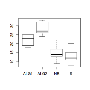
library(vcd) fit <- goodfit(day$BARNACLE, type='poisson') summary(fit)
Goodness-of-fit test for poisson distribution X^2 df P(> X^2) Likelihood Ratio 32.19209 17 0.01424181rootogram(fit)
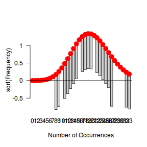
fit <- goodfit(day$BARNACLE, type='nbinom') summary(fit)
Goodness-of-fit test for nbinomial distribution X^2 df P(> X^2) Likelihood Ratio 18.41836 16 0.2999741rootogram(fit)
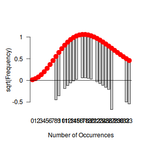
distplot(day$BARNACLE, type='poisson')
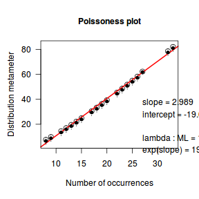
## Poisson would appear appropriate -
Fit the generalized linear model (GLM) relating the number of newly recruited barnacles to substrate type.
$$log(\mu) = \beta_0+\beta_1Treat_i+\epsilon_i, \hspace{1cm} \epsilon \sim Poisson(\lambda)$$
Show code
day.glm<-glm(BARNACLE~TREAT, family=poisson,data=day)
- Explore the patterns in simulated residuals:
Show code
library(DHARMa)
day.glm.sim <- simulateResiduals(day.glm) day.glm.sim
[1] "Class DHARMa with simulated residuals based on 250 simulations with refit = FALSE" [1] "see ?DHARMa::simulateResiduals for help" [1] "-----------------------------" [1] 0.848 0.288 0.220 0.564 0.740 0.196 0.784 0.360 0.376 0.748 0.048 0.292 0.668 0.488 0.948 0.356 [17] 0.072 0.660 0.968 0.288
plotSimulatedResiduals(day.glm.sim)
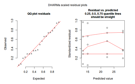
- Check the model for lack of fit via:
- Pearson Χ2
Show code
day.resid <- sum(resid(day.glm, type="pearson")^2) 1-pchisq(day.resid, day.glm$df.resid)
[1] 0.3641093
#No evidence of a lack of fit - Standardized residuals (plot)
Show code
plot(day.glm)
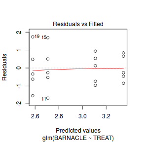
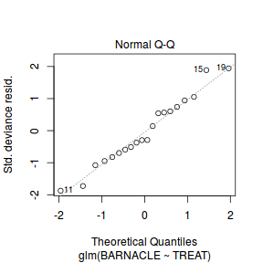
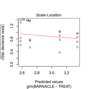
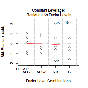
- Fitted and observed values (plot)
Show code
tempdata <- predict(day.glm, type='response', se=TRUE) tempdata <- cbind(day, Mean=tempdata[[1]], Lower=tempdata[[1]]-tempdata[[2]], Upper=tempdata[[1]]+tempdata[[2]]) library(ggplot2) ggplot(tempdata, aes(y=BARNACLE, x=TREAT)) + geom_boxplot() + geom_pointrange(aes(y=Mean, ymin=Lower, ymax=Upper), color='red')
## the fitted values (red point range) are not inconsistent with the observed counts - Kolmogorov-Smirnov uniformity test
Show code
testUniformity(day.glm.sim)
One-sample Kolmogorov-Smirnov test data: simulationOutput$scaledResiduals D = 0.124, p-value = 0.9182 alternative hypothesis: two-sided
- Pearson Χ2
- Estimate the dispersion parameter to evaluate over dispersion in the fitted model
- Via Pearson residuals
Show code
day.resid/day.glm$df.resid
[1] 1.083574
#No evidence of over dispersion - Via deviance
Show code
day.glm$deviance/day.glm$df.resid
[1] 1.075851
#No evidence of over dispersion - Via $\alpha$
Show code
library(AER) dispersiontest(day.glm)
Overdispersion test data: day.glm z = -0.58814, p-value = 0.7218 alternative hypothesis: true dispersion is greater than 1 sample estimates: dispersion 0.866859
- Simulated residuals
Show code
day.glm.sim <- simulateResiduals(day.glm, refit=T) testOverdispersion(day.glm.sim)
Overdispersion test via comparison to simulation under H0 data: day.glm.sim dispersion = 1.0786, p-value = 0.344 alternative hypothesis: overdispersion
## and overdispersion.. testZeroInflation(day.glm.sim)
Zero-inflation test via comparison to expected zeros with simulation under H0 data: day.glm.sim ratioObsExp = NaN, p-value < 2.2e-16 alternative hypothesis: more
- Via Pearson residuals
- Compare the expected number of zeros to the actual number of zeros to determine whether the model might be zero inflated.
- Calculate the proportion of zeros in the data
Show code
day.tab<-table(day$Count==0) day.tab/sum(day.tab)
numeric(0)
- Now work out the proportion of zeros we would expect from a Poisson distribution with a lambda equal to the mean count of day in this study.
Show codeClearly there are not more zeros than expected so the data are not zero inflated.
day.mu <- mean(day$Count) cnts <-rpois(1000,day.mu) day.tab<-table(cnts==0) day.tab/sum(day.tab)
numeric(0)
- Calculate the proportion of zeros in the data
- Explore the patterns in simulated residuals:
-
We can now test the null hypothesis that there is no effect of shore type on the abundance of striped day;
- Wald z-tests (these are equivalent to t-tests)
- Wald Chisq-test.
- Likelihood ratio test (LRT), analysis of deviance Chisq-tests (these are equivalent to ANOVA)
Show codesummary(day.glm)
Call: glm(formula = BARNACLE ~ TREAT, family = poisson, data = day) Deviance Residuals: Min 1Q Median 3Q Max -1.6748 -0.6522 -0.2630 0.5699 1.7380 Coefficients: Estimate Std. Error z value Pr(>|z|) (Intercept) 3.10906 0.09449 32.903 < 2e-16 *** TREATALG2 0.23733 0.12638 1.878 0.060387 . TREATNB -0.40101 0.14920 -2.688 0.007195 ** TREATS -0.52884 0.15518 -3.408 0.000654 *** --- Signif. codes: 0 '***' 0.001 '**' 0.01 '*' 0.05 '.' 0.1 ' ' 1 (Dispersion parameter for poisson family taken to be 1) Null deviance: 54.123 on 19 degrees of freedom Residual deviance: 17.214 on 16 degrees of freedom AIC: 120.34 Number of Fisher Scoring iterations: 4Show codelibrary(car) Anova(day.glm,test.statistic="Wald")
Analysis of Deviance Table (Type II tests) Response: BARNACLE Df Chisq Pr(>Chisq) TREAT 3 36.041 7.342e-08 *** Residuals 16 --- Signif. codes: 0 '***' 0.001 '**' 0.01 '*' 0.05 '.' 0.1 ' ' 1Show codeday.glmN <- glm(BARNACLE~1, family=poisson, data=day) anova(day.glmN, day.glm, test="Chisq")
Analysis of Deviance Table Model 1: BARNACLE ~ 1 Model 2: BARNACLE ~ TREAT Resid. Df Resid. Dev Df Deviance Pr(>Chi) 1 19 54.123 2 16 17.214 3 36.909 4.81e-08 *** --- Signif. codes: 0 '***' 0.001 '**' 0.01 '*' 0.05 '.' 0.1 ' ' 1
# OR anova(day.glm, test="Chisq")
Analysis of Deviance Table Model: poisson, link: log Response: BARNACLE Terms added sequentially (first to last) Df Deviance Resid. Df Resid. Dev Pr(>Chi) NULL 19 54.123 TREAT 3 36.909 16 17.214 4.81e-08 *** --- Signif. codes: 0 '***' 0.001 '**' 0.01 '*' 0.05 '.' 0.1 ' ' 1# OR Anova(day.glm, test.statistic="LR")
Analysis of Deviance Table (Type II tests) Response: BARNACLE LR Chisq Df Pr(>Chisq) TREAT 36.909 3 4.81e-08 *** --- Signif. codes: 0 '***' 0.001 '**' 0.01 '*' 0.05 '.' 0.1 ' ' 1 -
Lets now get the confidence intervals for the parameter estimates. Note these are still on the logs scale!
Show code
library(gmodels) ci(day.glm)
Estimate CI lower CI upper Std. Error p-value (Intercept) 3.1090610 2.90874874 3.30937318 0.09449112 1.977474e-237 TREATALG2 0.2373282 -0.03057639 0.50523276 0.12637573 6.038705e-02 TREATNB -0.4010108 -0.71730958 -0.08471194 0.14920422 7.195385e-03 TREATS -0.5288441 -0.85780588 -0.19988237 0.15517757 6.544249e-04
- Although we have now established that there is a statistical difference between the group means,
we do not yet know which group(s) are different from which other(s).
For this data a Tukey's multiple comparison test (to determine which surface
type groups are different from each other, in terms of number of barnacles)
could be appropriate.
Show code
library(multcomp) summary(glht(day.glm,linfct=mcp(TREAT="Tukey")))
Simultaneous Tests for General Linear Hypotheses Multiple Comparisons of Means: Tukey Contrasts Fit: glm(formula = BARNACLE ~ TREAT, family = poisson, data = day) Linear Hypotheses: Estimate Std. Error z value Pr(>|z|) ALG2 - ALG1 == 0 0.2373 0.1264 1.878 0.23536 NB - ALG1 == 0 -0.4010 0.1492 -2.688 0.03547 * S - ALG1 == 0 -0.5288 0.1552 -3.408 0.00363 ** NB - ALG2 == 0 -0.6383 0.1427 -4.472 < 0.001 *** S - ALG2 == 0 -0.7662 0.1490 -5.143 < 0.001 *** S - NB == 0 -0.1278 0.1688 -0.757 0.87234 --- Signif. codes: 0 '***' 0.001 '**' 0.01 '*' 0.05 '.' 0.1 ' ' 1 (Adjusted p values reported -- single-step method) -
I am now in the mood to derive other parameters from the model:
- Cell (population) means
Show codeOr the long way
day.means <- predict(day.glm,newdata=data.frame(TREAT=levels(day$TREAT)),se=T) day.means <- data.frame(day.means[1],day.means[2]) rownames(day.means) <- levels(day$TREAT) day.ci <- qt(0.975,day.glm$df.residual)*day.means[,2] day.means <- data.frame(day.means,lwr=day.means[,1]-day.ci,upr=day.means[,1]+day.ci) #On the scale of the response day.means <- predict(day.glm,newdata=data.frame(TREAT=levels(day$TREAT)),se=T, type="response") day.means <- data.frame(day.means[1],day.means[2]) rownames(day.means) <- levels(day$TREAT) day.ci <- qt(0.975,day.glm$df.residual)*day.means[,2] day.means <- data.frame(day.means,lwr=day.means[,1]-day.ci,upr=day.means[,1]+day.ci) day.means
fit se.fit lwr upr ALG1 22.4 2.116601 17.913006 26.88699 ALG2 28.4 2.383275 23.347683 33.45232 NB 15.0 1.732051 11.328217 18.67178 S 13.2 1.624807 9.755563 16.64444
opar<-par(mar=c(4,5,1,1)) plot(BARNACLE~as.numeric(TREAT), data=day, ann=F, axes=F, type="n") points(BARNACLE~as.numeric(TREAT), data=day, pch=16, col="grey80") arrows(as.numeric(factor(rownames(day.means))),day.means$lwr,as.numeric(factor(rownames(day.means))), day.means$upr, ang=90, length=0.1, code=3) points(day.means$fit~as.numeric(factor(rownames(day.means))), pch=16) axis(1, at=as.numeric(factor(rownames(day.means))), labels=rownames(day.means)) mtext("Treatment",1, line=3, cex=1.2) axis(2, las=1) mtext("Number of newly recruited barnacles",2, line=3, cex=1.2) box(bty="l")
 Show code
#On a link (log) scale cmat <- cbind(c(1,0,0,0),c(1,1,0,0),c(1,0,1,0),c(1,0,0,1)) day.mu<-t(day.glm$coef %*% cmat) day.se <- sqrt(diag(t(cmat) %*% vcov(day.glm) %*% cmat)) day.means <- data.frame(fit=day.mu,se=day.se) rownames(day.means) <- levels(day$TREAT) day.ci <- qt(0.975,day.glm$df.residual)*day.se day.means <- data.frame(day.means,lwr=day.mu-day.ci,upr=day.mu+day.ci) #On a response scale cmat <- cbind(c(1,0,0,0),c(1,1,0,0),c(1,0,1,0),c(1,0,0,1)) day.mu<-t(day.glm$coef %*% cmat) day.se <- sqrt(diag(t(cmat) %*% vcov(day.glm) %*% cmat))*abs(poisson()$mu.eta(day.mu)) day.mu<-exp(day.mu) #OR day.se <- sqrt(diag(vcov(day.glm) %*% cmat))*day.mu day.means <- data.frame(fit=day.mu,se=day.se) rownames(day.means) <- levels(day$TREAT) day.ci <- qt(0.975,day.glm$df.residual)*day.se day.means <- data.frame(day.means,lwr=day.mu-day.ci,upr=day.mu+day.ci) day.means
fit se lwr upr ALG1 22.4 2.116601 17.913006 26.88699 ALG2 28.4 2.383275 23.347683 33.45232 NB 15.0 1.732051 11.328217 18.67178 S 13.2 1.624807 9.755563 16.64444
- Differences between each treatment mean and the global mean
Show code
#On a link (log) scale cmat <- rbind(c(1,0,0,0),c(1,1,0,0),c(1,0,1,0),c(1,0,0,1)) gm.cmat <-apply(cmat,2,mean) for (i in 1:nrow(cmat)){ cmat[i,]<-cmat[i,]-gm.cmat } #Grand Mean day.glm$coef %*% gm.cmat
[,1] [1,] 2.935929
#Effect sizes day.mu<-t(day.glm$coef %*% t(cmat)) day.se <- sqrt(diag(cmat %*% vcov(day.glm) %*% t(cmat))) day.means <- data.frame(fit=day.mu,se=day.se) rownames(day.means) <- levels(day$TREAT) day.ci <- qt(0.975,day.glm$df.residual)*day.se day.means <- data.frame(day.means,lwr=day.mu-day.ci,upr=day.mu+day.ci) day.means
fit se lwr upr ALG1 0.1731317 0.08510443 -0.007281663 0.3535450 ALG2 0.4104599 0.07937005 0.242202862 0.5787169 NB -0.2278791 0.09718613 -0.433904466 -0.0218537 S -0.3557125 0.10175575 -0.571425004 -0.1399999
#On a response scale cmat <- rbind(c(1,0,0,0),c(1,1,0,0),c(1,0,1,0),c(1,0,0,1)) gm.cmat <-apply(cmat,2,mean) for (i in 1:nrow(cmat)){ cmat[i,]<-cmat[i,]-gm.cmat } #Grand Mean day.glm$coef %*% gm.cmat
[,1] [1,] 2.935929
#Effect sizes day.mu<-t(day.glm$coef %*% t(cmat)) day.se <- sqrt(diag(cmat %*% vcov(day.glm) %*% t(cmat)))*abs(poisson()$mu.eta(day.mu)) day.mu<-exp(abs(day.mu)) day.means <- data.frame(fit=day.mu,se=day.se) rownames(day.means) <- levels(day$TREAT) day.ci <- qt(0.975,day.glm$df.residual)*day.se day.means <- data.frame(day.means,lwr=day.mu-day.ci,upr=day.mu+day.ci) day.means
fit se lwr upr ALG1 1.189023 0.10119110 0.9745071 1.403538 ALG2 1.507511 0.11965122 1.2538616 1.761160 NB 1.255933 0.07738159 1.0918918 1.419975 S 1.427197 0.07129761 1.2760529 1.578341
#estimable(day.glm,cm=cmat) #confint(day.glm)
- Cell (population) means
- To standardize the moth counts for transect section length, we could convert the counts into densities (by dividing the A by METERS.
Create such as variable (DENSITY and explore the usual ANOVA assumptions.
Show code
moths <- within(moths, DENSITY<-A/METERS) boxplot(DENSITY~HABITAT, data=moths)
library(vcd) fit <- goodfit(moths$A, type='poisson') summary(fit)
Goodness-of-fit test for poisson distribution X^2 df P(> X^2) Likelihood Ratio 170.2708 11 1.037761e-30rootogram(fit)
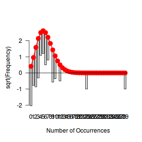
fit <- goodfit(moths$A, type='nbinom') summary(fit)
Goodness-of-fit test for nbinomial distribution X^2 df P(> X^2) Likelihood Ratio 32.1636 10 0.0003760562rootogram(fit)
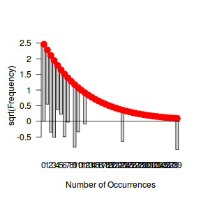
Ord_plot(moths$A, tol=0.2)
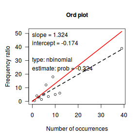
distplot(moths$A, type='poisson')
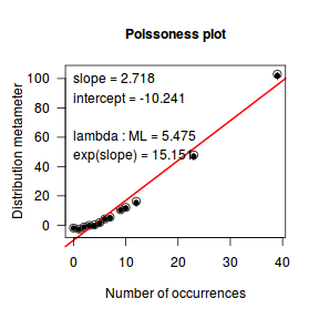
distplot(moths$A, type='nbinom')
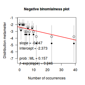
- Clearly, the there is an issue with normality and homogeneity of variance. Perhaps it would be worth transforming
density in an attempt to normalize these data. Given that there are densities of zero, a straight logarithmic transformation would not be appropriate.
Alternatives could inlude a square-root transform, a forth-root transform and a log plus 1 transform.
Show code
moths <- within(moths, DENSITY<-A/METERS) boxplot(sqrt(DENSITY)~HABITAT, data=moths)
boxplot((DENSITY)^0.25~HABITAT, data=moths)
boxplot(log(DENSITY+1)~HABITAT, data=moths)
- Arguably, non of the above transformations have improved the data's adherence to the linear modelling assumptions.
Count data (such as the abundance of moth species A) is unlikely to follow a normal or even log-normal distribution. Count data
are usually more appropriately modelled via a Poisson or Negative binomial distributions. Note, dividing by transect length is unlikely to alter
the underlying nature of the data distribution as it still based on counts.
Fit the generalized linear model (GLM) relating the number of newly recruited barnacles to substrate type.
$$log(\mu) = \beta_0+\beta_1 Habitat_i+\epsilon_i, \hspace{1cm} \epsilon \sim Poisson(\lambda)\\
log(\mu) = \beta_0+\beta_1 Habitat_i+\epsilon_i, \hspace{1cm} \epsilon \sim NB(n,p)
$$
Show code
moths.glm <- glm(A~HABITAT, data=moths, family=poisson) library(MASS) moths.glmNB <- glm.nb(A~HABITAT, data=moths)
- Actually, the above models fail to account for the length of the section of transect.
We could do this a couple of ways:
- Add METERS as a covariate. Note, since we are modelling against a Poission distribution with a log link function,
we should also log the covariate - in order to maintain linearity between the expected value of species A abundance and transect length.
$$log(\mu) = \beta_0+\beta_1 Habitat_i + \beta_2 log(meters) +\epsilon_i, \hspace{1cm} \epsilon \sim Poisson(\lambda)\\
log(\mu) = \beta_0+\beta_1 Habitat_i + \beta_2 log(meters) +\epsilon_i, \hspace{1cm} \epsilon \sim NB(n,p)
$$
Show code
moths.glmC <- glm(A~log(METERS)+HABITAT, data=moths, family=poisson) moths.glmNBC <- glm.nb(A~log(METERS)+HABITAT, data=moths)
- Add METERS as an offset in which case $\beta_2$ is assumed to be 1 (a reasonable assumption in this case).
The advantage is that it does not sacrifice any residual degrees of freedom. Again to maintain linearity, the offset should include
the log of transect length.
$$log(\mu) = \beta_0+\beta_1 Habitat_i + log(meters) +\epsilon_i, \hspace{1cm} \epsilon \sim Poisson(\lambda)\\
log(\mu) = \beta_0+\beta_1 Habitat_i + log(meters) +\epsilon_i, \hspace{1cm} \epsilon \sim NB(n,p)$$
Show code
moths.glmO <- glm(A~HABITAT, offset=log(METERS), data=moths, family=poisson) moths.glmNBO <- glm.nb(A~HABITAT+offset(log(METERS)), data=moths)
- Add METERS as a covariate. Note, since we are modelling against a Poission distribution with a log link function,
we should also log the covariate - in order to maintain linearity between the expected value of species A abundance and transect length.
$$log(\mu) = \beta_0+\beta_1 Habitat_i + \beta_2 log(meters) +\epsilon_i, \hspace{1cm} \epsilon \sim Poisson(\lambda)\\
log(\mu) = \beta_0+\beta_1 Habitat_i + \beta_2 log(meters) +\epsilon_i, \hspace{1cm} \epsilon \sim NB(n,p)
$$
- Lets explore the simulated residuals for each of the above models
Show code
library(DHARMa) # moths.glm A~HABITAT (Poisson) moths.glm.sim <- simulateResiduals(moths.glm) plotSimulatedResiduals(moths.glm.sim)
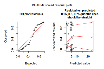
# moths.glmNB A~HABITAT (NegBin) moths.glmNB.sim <- simulateResiduals(moths.glmNB) plotSimulatedResiduals(moths.glmNB.sim)
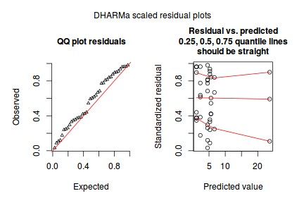
# moths.glmC A~log(METERS) +HABITAT (Poisson) moths.glmC.sim <- simulateResiduals(moths.glmC) plotSimulatedResiduals(moths.glmC.sim)
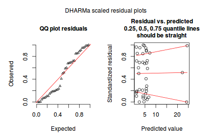
# moths.glmNBC A~log(METERS) +HABITAT (NegBin) moths.glmNBC.sim <- simulateResiduals(moths.glmNBC) plotSimulatedResiduals(moths.glmNBC.sim)
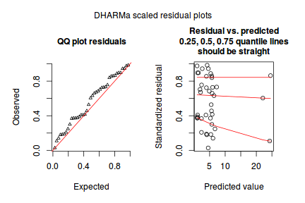
# moths.glmO A~ HABITAT,offset=log(METERS) (Poisson) moths.glmO.sim <- simulateResiduals(moths.glmO) plotSimulatedResiduals(moths.glmO.sim)
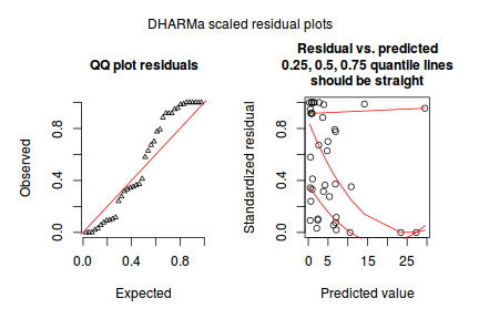
# moths.glmNBO A~HABITAT, offset=log(METERS) (NegBin) moths.glmNBO.sim <- simulateResiduals(moths.glmNBO) plotSimulatedResiduals(moths.glmNBO.sim)
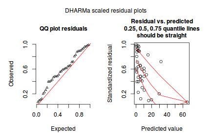
- Check the model for lack of fit via:
- Pearson Χ2
Show code
## When Meters added as a covariate moths.residC <- sum(resid(moths.glmC, type="pearson")^2) 1-pchisq(moths.residC, moths.glmC$df.resid)
[1] 6.735895e-07
#Clear evidence of a lack of fit moths.residNBC <- sum(resid(moths.glmNBC, type="pearson")^2) 1-pchisq(moths.residNBC, moths.glmNBC$df.resid)
[1] 0.175419
#No evidence of a lack of fit ## When Meters added as an offset moths.residO <- sum(resid(moths.glmO, type="pearson")^2) 1-pchisq(moths.residO, moths.glmO$df.resid)
[1] 0
#Clear evidence of a lack of fit moths.residNBO <- sum(resid(moths.glmNBO, type="pearson")^2) 1-pchisq(moths.residNBO, moths.glmNBO$df.resid)
[1] 0.04489437
#Some evidence of a lack of fit ##Hence it appears that the NB model that incorporates Meters as ## a covariate is the best fit
- Standardized residuals (plot)
Show code
## Meters as covariate plot(moths.glmC)
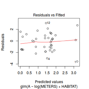
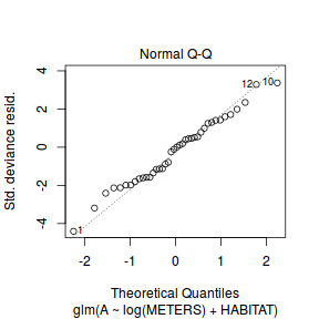
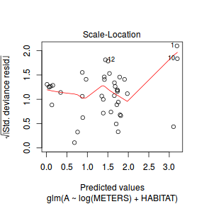
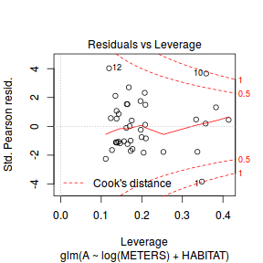
plot(resid(moths.glmC, type="pearson") ~ fitted(moths.glmC))
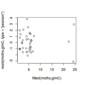
plot(resid(moths.glmC, type="pearson") ~ predict(moths.glmC, type="link"))
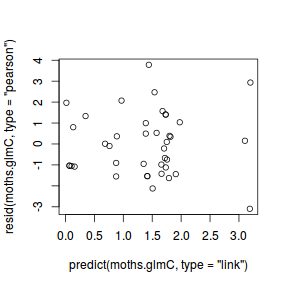
## Meters as offset plot(moths.glmO)
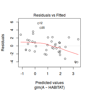
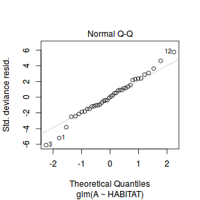
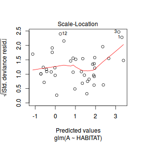
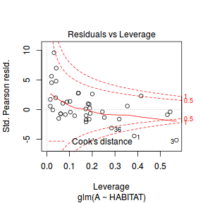
plot(resid(moths.glmO, type="pearson") ~ fitted(moths.glmO))
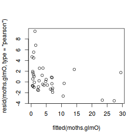
plot(resid(moths.glmO, type="pearson") ~ predict(moths.glmO, type="link"))
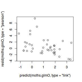
## Meters as a covariate plot(moths.glmNBC)
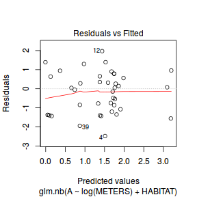
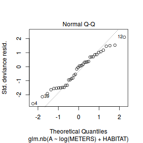
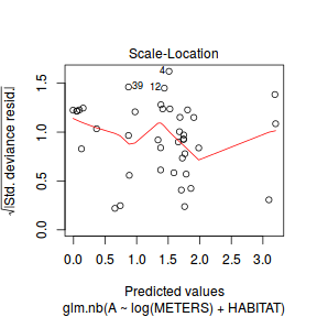
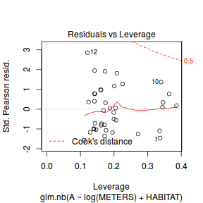
plot(resid(moths.glmNBC, type="pearson") ~ fitted(moths.glmNBC))
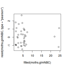
plot(resid(moths.glmNBC, type="pearson") ~ predict(moths.glmNBC, type="link"))
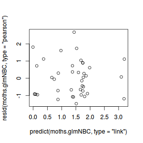
## Meters as an offset plot(moths.glmNBO)
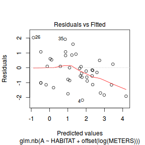
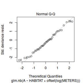
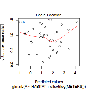
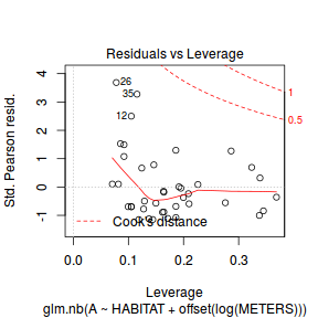
plot(resid(moths.glmNBO, type="pearson") ~ fitted(moths.glmNBO))
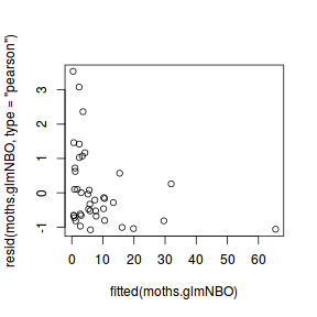
plot(resid(moths.glmNBO, type="pearson") ~ predict(moths.glmNBO, type="link"))
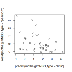
## Clearly the models in which Meters has been incorporated ## as an offset still have patterns in the residuals. This is likely ## to be the result of the offset assuming a 1:1 relationship between ## Moth abundance and Meters when the slope of this relationship is not ## equal to 1 and thus there is still drift in the response. ## Incorporating Meters as a full covariate does ## account for the drift observed.
- Fitted and observed values (plot)
Show code
## Meters as a covariate newdata <- data.frame(HABITAT = moths$HABITAT, METERS=mean(moths$METERS)) tempdata <- predict(moths.glmC, newdata=newdata, type='response', se=TRUE) tempdata <- cbind(moths, Mean=tempdata[[1]], Lower=tempdata[[1]]-tempdata[[2]], Upper=tempdata[[1]]+tempdata[[2]]) library(ggplot2) ggplot(tempdata, aes(y=A, x=HABITAT)) + geom_boxplot() + geom_pointrange(aes(y=Mean, ymin=Lower, ymax=Upper), color='red')
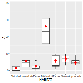
newdata <- data.frame(HABITAT = moths$HABITAT, METERS=mean(moths$METERS)) tempdata <- predict(moths.glmNBC, newdata=newdata, type='response', se=TRUE) tempdata <- cbind(moths, Mean=tempdata[[1]], Lower=tempdata[[1]]-tempdata[[2]], Upper=tempdata[[1]]+tempdata[[2]]) library(ggplot2) ggplot(tempdata, aes(y=A, x=HABITAT)) + geom_boxplot() + geom_pointrange(aes(y=Mean, ymin=Lower, ymax=Upper), color='red')
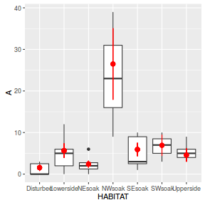
## When Meters added as an offset newdata <- data.frame(HABITAT = moths$HABITAT, METERS=mean(moths$METERS)) tempdata <- predict(moths.glmO, newdata=newdata, type='response', se=TRUE) tempdata <- cbind(moths, Mean=tempdata[[1]], Lower=tempdata[[1]]-tempdata[[2]], Upper=tempdata[[1]]+tempdata[[2]]) library(ggplot2) ggplot(tempdata, aes(y=A, x=HABITAT)) + geom_boxplot() + geom_pointrange(aes(y=Mean, ymin=Lower, ymax=Upper), color='red')
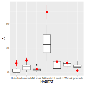
newdata <- data.frame(HABITAT = moths$HABITAT, METERS=mean(moths$METERS)) tempdata <- predict(moths.glmNBO, newdata=newdata, type='response', se=TRUE) tempdata <- cbind(moths, Mean=tempdata[[1]], Lower=tempdata[[1]]-tempdata[[2]], Upper=tempdata[[1]]+tempdata[[2]]) library(ggplot2) ggplot(tempdata, aes(y=A, x=HABITAT)) + geom_boxplot() + geom_pointrange(aes(y=Mean, ymin=Lower, ymax=Upper), color='red')
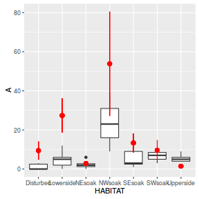
## the model does not appear to be all that accurate, most of the treatment levels are ## either over or underestimated. It might be worth pursuing the Negative Binomial model.
- Kolmogorov-Smirnov uniformity test
Show code
# moths.glm A~HABITAT (Poisson) moths.glm.sim <- simulateResiduals(moths.glm) testUniformity(moths.glm.sim)
One-sample Kolmogorov-Smirnov test data: simulationOutput$scaledResiduals D = 0.201, p-value = 0.07895 alternative hypothesis: two-sided
# moths.glmNB A~HABITAT (NegBin) moths.glmNB.sim <- simulateResiduals(moths.glmNB) testUniformity(moths.glmNB.sim)
One-sample Kolmogorov-Smirnov test data: simulationOutput$scaledResiduals D = 0.134, p-value = 0.4691 alternative hypothesis: two-sided
# moths.glmC A~log(METERS) +HABITAT (Poisson) moths.glmC.sim <- simulateResiduals(moths.glmC) testUniformity(moths.glmC.sim)
One-sample Kolmogorov-Smirnov test data: simulationOutput$scaledResiduals D = 0.172, p-value = 0.1874 alternative hypothesis: two-sided
# moths.glmNBC A~log(METERS) +HABITAT (NegBin) moths.glmNBC.sim <- simulateResiduals(moths.glmNBC) testUniformity(moths.glmNBC.sim)
One-sample Kolmogorov-Smirnov test data: simulationOutput$scaledResiduals D = 0.158, p-value = 0.2708 alternative hypothesis: two-sided
# moths.glmO A~ HABITAT,offset=log(METERS) (Poisson) moths.glmO.sim <- simulateResiduals(moths.glmO) testUniformity(moths.glmO.sim)
One-sample Kolmogorov-Smirnov test data: simulationOutput$scaledResiduals D = 0.215, p-value = 0.04955 alternative hypothesis: two-sided
# moths.glmNBO A~HABITAT, offset=log(METERS) (NegBin) moths.glmNBO.sim <- simulateResiduals(moths.glmNBO) testUniformity(moths.glmNBO.sim)
One-sample Kolmogorov-Smirnov test data: simulationOutput$scaledResiduals D = 0.204, p-value = 0.07163 alternative hypothesis: two-sided
- Estimate the dispersion parameter to evaluate over dispersion in the fitted model
- Via Pearson residuals
Show code
moths.residC/moths.glmC$df.resid
[1] 2.700801
moths.residNBC/moths.glmNBC$df.resid
[1] 1.228093
moths.residO/moths.glmO$df.resid
[1] 8.843367
moths.residNBO/moths.glmNBO$df.resid
[1] 1.452578
## Poisson models have some evidence of overdispersion ## (particularly the model that incorporates Meters as an offset).
- Via deviance
Show code
moths.glmC$deviance/moths.glmC$df.resid
[1] 2.93723
moths.glmO$deviance/moths.glmO$df.resid
[1] 5.462792
moths.glmNBC$deviance/moths.glmNBC$df.resid
[1] 1.455681
moths.glmNBO$deviance/moths.glmNBO$df.resid
[1] 1.371939
## Poisson models have some evidence of overdispersion ## (particularly the model that incorporates Meters as an offset).
- Via $\alpha$
Show code
library(AER) dispersiontest(moths.glmC)
Overdispersion test data: moths.glmC z = 2.6752, p-value = 0.003735 alternative hypothesis: true dispersion is greater than 1 sample estimates: dispersion 2.165306
- Simulated residuals
Show code
# moths.glm A~HABITAT (Poisson) moths.glm.sim <- simulateResiduals(moths.glm, refit=T) testOverdispersion(moths.glm.sim)
Overdispersion test via comparison to simulation under H0 data: moths.glm.sim dispersion = 2.7082, p-value < 2.2e-16 alternative hypothesis: overdispersion
testZeroInflation(moths.glm.sim)
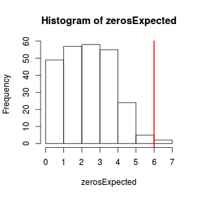
Zero-inflation test via comparison to expected zeros with simulation under H0 data: moths.glm.sim ratioObsExp = 2.1186, p-value = 0.008 alternative hypothesis: more
# moths.glmNB A~HABITAT (NegBin) moths.glmNB.sim <- simulateResiduals(moths.glmNB, refit=T) testOverdispersion(moths.glmNB.sim)
Overdispersion test via comparison to simulation under H0 data: moths.glmNB.sim dispersion = 0.99928, p-value = 0.48 alternative hypothesis: overdispersion
testZeroInflation(moths.glmNB.sim)
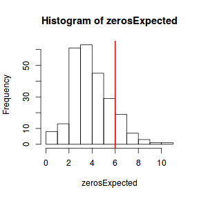
Zero-inflation test via comparison to expected zeros with simulation under H0 data: moths.glmNB.sim ratioObsExp = 1.3599, p-value = 0.124 alternative hypothesis: more
# moths.glmC A~log(METERS) +HABITAT (Poisson) moths$logMETERS <- moths$METERS moths.glmC <- glm(A~logMETERS+HABITAT, data=moths, family=poisson) moths.glmC.sim <- simulateResiduals(moths.glmC, refit=T) testOverdispersion(moths.glmC.sim)
Overdispersion test via comparison to simulation under H0 data: moths.glmC.sim dispersion = 2.6677, p-value < 2.2e-16 alternative hypothesis: overdispersion
testZeroInflation(moths.glmC.sim)
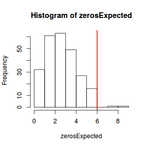
Zero-inflation test via comparison to expected zeros with simulation under H0 data: moths.glmC.sim ratioObsExp = 1.9206, p-value = 0.008 alternative hypothesis: more
# moths.glmNBC A~log(METERS) +HABITAT (NegBin) moths.glmNBC <- glm.nb(A~logMETERS+HABITAT, data=moths) moths.glmNBC.sim <- simulateResiduals(moths.glmNBC, refit=T) testOverdispersion(moths.glmNBC.sim)
Overdispersion test via comparison to simulation under H0 data: moths.glmNBC.sim dispersion = 1.0051, p-value = 0.456 alternative hypothesis: overdispersion
testZeroInflation(moths.glmNBC.sim)
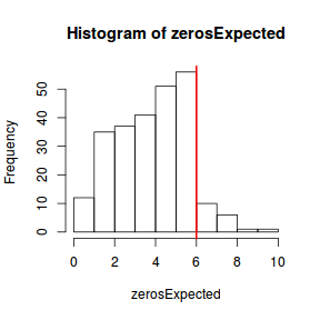
Zero-inflation test via comparison to expected zeros with simulation under H0 data: moths.glmNBC.sim ratioObsExp = 1.385, p-value = 0.072 alternative hypothesis: more
# moths.glmO A~ HABITAT,offset=log(METERS) (Poisson) moths.glmO <- glm(A~HABITAT, offset=logMETERS, data=moths, family=poisson)
Error in glm.fit(x = structure(c(1, 1, 1, 1, 1, 1, 1, 1, 1, 1, 1, 1, 1, : NA/NaN/Inf in 'x'
moths.glmO.sim <- simulateResiduals(moths.glmO, refit=T)
Error in eval(expr, envir, enclos): object 'METERS' not found
testOverdispersion(moths.glmO.sim)
Error in testOverdispersion(moths.glmO.sim): Overdispersion test requires simulated residuals with refit = T
testZeroInflation(moths.glmO.sim)
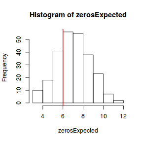
Zero-inflation test via comparison to expected zeros with simulation under H0 data: moths.glmO.sim ratioObsExp = 0.79872, p-value = 0.724 alternative hypothesis: more
# moths.glmNBO A~HABITAT, offset=log(METERS) (NegBin) moths.glmNBO <- glm.nb(A~HABITAT, offset=logMETERS, data=moths)
Error in glm.control(...): object 'logMETERS' not found
moths.glmNBO.sim <- simulateResiduals(moths.glmNBO, refit=T)
Error in offset(log(METERS)): object 'METERS' not found
testOverdispersion(moths.glmNBO.sim)
Error in testOverdispersion(moths.glmNBO.sim): Overdispersion test requires simulated residuals with refit = T
testZeroInflation(moths.glmNBO.sim)
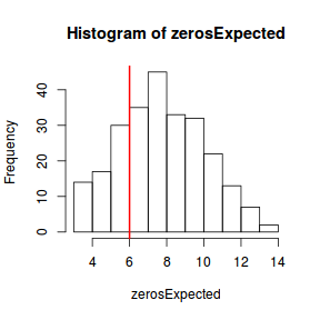
Zero-inflation test via comparison to expected zeros with simulation under H0 data: moths.glmNBO.sim ratioObsExp = 0.72922, p-value = 0.756 alternative hypothesis: more
- Compare the expected number of zeros to the actual number of zeros to determine whether the model might be zero inflated.
- Calculate the proportion of zeros in the data
Show code
moths.tab<-table(moths$A==0) moths.tab/sum(moths.tab)
FALSE TRUE 0.85 0.15
- Now work out the proportion of zeros we would expect from a Poisson distribution with a lambda equal to the mean count of moths in this study.
Show codeClearly there are more zeros than expected so the data. However, as the excess is not really high ($>40%$), the Negative Binomial is likely to have been sufficient to account for this level of zero-inflation.
moths.mu <- mean(moths$A) cnts <-rpois(1000,moths.mu) moths.tab<-table(cnts==0) moths.tab/sum(moths.tab)
FALSE TRUE 0.994 0.006
- We might expect that the Negative Binomial model with Meters incorporated as a covariate will be the most parsimonious model. Check whether this is the case.
Show codelibrary(MuMIn) AICc(moths.glmO, moths.glmC, moths.glmNBO, moths.glmNBC)
df AICc moths.glmO 7 312.4946 moths.glmC 8 230.6100 moths.glmNBO 8 233.1423 moths.glmNBC 9 213.8393
- It seems reasonable to conclude that the candidate model containing Meter as a full covariate and Negative Binomial distribution is the most appropriate. Lets now explore the model summary.
Show codesummary(moths.glmNBC)
Call: glm.nb(formula = A ~ logMETERS + HABITAT, data = moths, init.theta = 4.073590567, link = log) Deviance Residuals: Min 1Q Median 3Q Max -2.44044 -1.09751 -0.08035 0.60782 1.89729 Coefficients: Estimate Std. Error z value Pr(>|z|) (Intercept) 0.111029 0.401674 0.276 0.78223 logMETERS 0.002777 0.004220 0.658 0.51041 HABITATLowerside 1.340081 0.465311 2.880 0.00398 ** HABITATNEsoak 0.604008 0.545287 1.108 0.26800 HABITATNWsoak 2.991684 0.510033 5.866 4.47e-09 *** HABITATSEsoak 1.478376 0.479789 3.081 0.00206 ** HABITATSWsoak 1.672233 0.557448 3.000 0.00270 ** HABITATUpperside 1.097219 0.925028 1.186 0.23556 --- Signif. codes: 0 '***' 0.001 '**' 0.01 '*' 0.05 '.' 0.1 ' ' 1 (Dispersion parameter for Negative Binomial(4.0736) family taken to be 1) Null deviance: 104.368 on 39 degrees of freedom Residual deviance: 46.675 on 32 degrees of freedom AIC: 207.84 Number of Fisher Scoring iterations: 1 Theta: 4.07 Std. Err.: 1.88 2 x log-likelihood: -189.839## Since paramters are on a log scale, care must be taken when interpreting coefficients. ## Normally treatment contrasts are interpreted as the difference between each group and the first ## treatment level (in this case Disturb). When coefficients are on a log scale, the back transformed ## coefficients are interpreted as ratios of each group to the first level. ## For example, the coefficient for HABITATLowerside (1.2864) equates to a ratio of 3.62 ## (after exponentiation). Hence we would conclude that moths are 3.63 times more abundant ## in the Lowerside habitat than the Disturb habitat.
- Figure time - Oh yer...
Show codenewdata <- data.frame(HABITAT=levels(moths$HABITAT), METER=mean(moths$METER)) Xmat <- model.matrix(~log(METER)+HABITAT, data=newdata) coefs <- coef(moths.glmNBC) fit <- as.vector(coefs %*% t(Xmat)) se <- sqrt(diag(Xmat %*% vcov(moths.glmNBC) %*% t(Xmat))) q <- qt(0.975, df=moths.glmNBC$df.residual) newdata <- cbind(newdata, fit=exp(fit), lower=exp(fit-q*se), upper=exp(fit+q*se)) head(newdata)
HABITAT METER fit lower upper 1 Disturbed 45.5 1.129338 0.4992001 2.554896 2 Lowerside 45.5 4.313339 2.6398783 7.047634 3 NEsoak 45.5 2.066051 0.9605008 4.444107 4 NWsoak 45.5 22.495505 11.7518090 43.061262 5 SEsoak 45.5 4.953070 2.8630166 8.568898 6 SWsoak 45.5 6.012642 2.7014491 13.382397
ggplot(newdata, aes(y=fit, x=HABITAT)) + geom_pointrange(aes(ymin=lower, ymax=upper)) + theme_classic()
Poisson t-test with overdispersion
The same marine ecologist that featured earlier was also interested in examining the effects of wave exposure on the abundance of another intertidal marine limpet Cellana tramoserica on rocky intertidal shores. Again, a single quadrat was placed on 10 exposed (to large waves) shores and 10 sheltered shores. From each quadrat, the number of smooth limpets (Cellana tramoserica) were counted.
Download LimpetsSmooth data setFormat of limpetsSmooth.csv data files Count Shore 4 sheltered 1 sheltered 2 sheltered 0 sheltered 4 sheltered ... ... Shore Categorical description of the shore type (sheltered or exposed) - Predictor variable Count Number of limpets per quadrat - Response variable 
Open the limpetsSmooth data set.
Show codelimpets <- read.table('../downloads/data/limpetsSmooth.csv', header=T, sep=',', strip.white=T) limpets
Count Shore 1 3 sheltered 2 1 sheltered 3 6 sheltered 4 0 sheltered 5 4 sheltered 6 3 sheltered 7 8 sheltered 8 1 sheltered 9 13 sheltered 10 0 sheltered 11 2 exposed 12 14 exposed 13 2 exposed 14 3 exposed 15 31 exposed 16 1 exposed 17 13 exposed 18 8 exposed 19 14 exposed 20 11 exposed
-
We might have initially have been tempted to perform a simple t-test on these data.
However, as the response are counts (and close to zero), lets instead fit the same model with a Poisson distribution.
$$log(\mu) = \beta_0+\beta1Shore_i+\epsilon_i, \hspace{1cm} \epsilon \sim Poisson(\lambda)$$
Show code
limpets.glm <- glm(Count~Shore, family=poisson, data=limpets)
- Check the model for lack of fit via:
- Pearson Χ2
Show code
limpets.resid <- sum(resid(limpets.glm, type="pearson")^2) 1-pchisq(limpets.resid, limpets.glm$df.resid)
[1] 4.440892e-16
#Evidence of a lack of fit - Deviance (G2)
Show code
1-pchisq(limpets.glm$deviance, limpets.glm$df.resid)
[1] 1.887379e-15
#Evidence of a lack of fit - Standardized residuals (plot)
Show code
plot(limpets.glm)
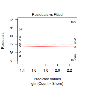
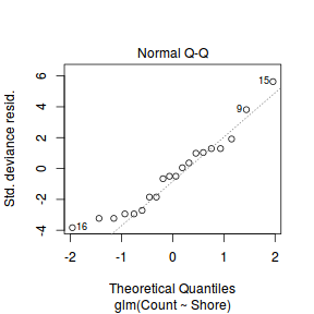
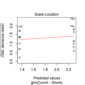
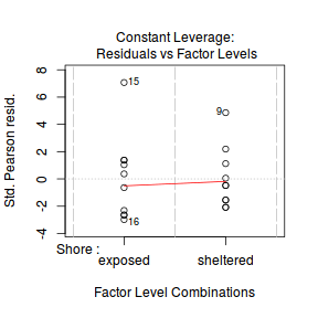
- Pearson Χ2
- Estimate the dispersion parameter to evaluate over dispersion in the fitted model
- Via Pearson residuals
Show code
limpets.resid/limpets.glm$df.resid
[1] 6.358197
#Evidence of over dispersion - Via deviance
Show code
limpets.glm$deviance/limpets.glm$df.resid
[1] 6.177846
#Evidence of over dispersion
- Via Pearson residuals
- Compare the expected number of zeros to the actual number of zeros to determine whether the model might be zero inflated.
- Calculate the proportion of zeros in the data
Show code
limpets.tab<-table(limpets$Count==0) limpets.tab/sum(limpets.tab)
FALSE TRUE 0.9 0.1
- Now work out the proportion of zeros we would expect from a Poisson distribution with a lambda equal to the mean count of limpets in this study.
Show codeThere is a suggestion that there are more zeros than we should expect given the means of each population. It may be that these data are zero inflated, however, given that our other diagnostics have suggested that the model itself might be inappropriate, zero inflation is not the primary concern.
limpets.mu <- mean(limpets$Count) cnts <-rpois(1000,limpets.mu) limpets.tab<-table(cnts==0) limpets.tab/sum(limpets.tab)
FALSE TRUE 0.999 0.001
- Calculate the proportion of zeros in the data
- Check the model for lack of fit via:
- As part of the routine exploratory data analysis:
- Explore the distribution of counts from each population
Show codeThere does appear to be some clumping which might suggest that there are other unmeasured influences.
boxplot(Count~Shore,data=limpets) rug(jitter(limpets$Count), side=2)
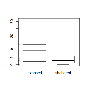
- Explore the distribution of counts from each population
-
There are generally two ways of handling this form of overdispersion.
- Fit the model with a quasipoisson distribution in which the dispersion factor (lambda) is not assumed to be 1.
The degree of variability (and how this differs from the mean) is estimated and the dispersion factor is incorporated.
Show code
limpets.glmQ <- glm(Count~Shore, family=quasipoisson, data=limpets)
- t-tests
- Wald F-test. Note that F = t2
Show codesummary(limpets.glmQ)
Call: glm(formula = Count ~ Shore, family = quasipoisson, data = limpets) Deviance Residuals: Min 1Q Median 3Q Max -3.6352 -2.6303 -0.4752 1.0449 5.3451 Coefficients: Estimate Std. Error t value Pr(>|t|) (Intercept) 2.2925 0.2534 9.046 4.08e-08 *** Shoresheltered -0.9316 0.4767 -1.954 0.0664 . --- Signif. codes: 0 '***' 0.001 '**' 0.01 '*' 0.05 '.' 0.1 ' ' 1 (Dispersion parameter for quasipoisson family taken to be 6.358223) Null deviance: 138.18 on 19 degrees of freedom Residual deviance: 111.20 on 18 degrees of freedom AIC: NA Number of Fisher Scoring iterations: 5Show codelibrary(car) Anova(limpets.glmQ,test.statistic="F")
Analysis of Deviance Table (Type II tests) Response: Count Error estimate based on Pearson residuals SS Df F Pr(>F) Shore 26.978 1 4.243 0.05417 . Residuals 114.448 18 --- Signif. codes: 0 '***' 0.001 '**' 0.01 '*' 0.05 '.' 0.1 ' ' 1#OR anova(limpets.glmQ,test="F")
Analysis of Deviance Table Model: quasipoisson, link: log Response: Count Terms added sequentially (first to last) Df Deviance Resid. Df Resid. Dev F Pr(>F) NULL 19 138.18 Shore 1 26.978 18 111.20 4.243 0.05417 . --- Signif. codes: 0 '***' 0.001 '**' 0.01 '*' 0.05 '.' 0.1 ' ' 1 - Fit the model with a negative binomial distribution (which accounts for the clumping).
Show codeCheck the fit
limpets.glmNB <- glm.nb(Count~Shore, data=limpets)
Show codelimpets.resid <- sum(resid(limpets.glmNB, type="pearson")^2) 1-pchisq(limpets.resid, limpets.glmNB$df.resid)
[1] 0.4333663
#Deviance 1-pchisq(limpets.glmNB$deviance, limpets.glmNB$df.resid)
[1] 0.215451
- Wald z-tests (these are equivalent to t-tests)
- Wald Chisq-test. Note that Chisq = z2
Show codesummary(limpets.glmNB)
Call: glm.nb(formula = Count ~ Shore, data = limpets, init.theta = 1.283382111, link = log) Deviance Residuals: Min 1Q Median 3Q Max -1.8929 -1.0926 -0.2313 0.3943 1.5320 Coefficients: Estimate Std. Error z value Pr(>|z|) (Intercept) 2.2925 0.2967 7.727 1.1e-14 *** Shoresheltered -0.9316 0.4377 -2.128 0.0333 * --- Signif. codes: 0 '***' 0.001 '**' 0.01 '*' 0.05 '.' 0.1 ' ' 1 (Dispersion parameter for Negative Binomial(1.2834) family taken to be 1) Null deviance: 26.843 on 19 degrees of freedom Residual deviance: 22.382 on 18 degrees of freedom AIC: 122.02 Number of Fisher Scoring iterations: 1 Theta: 1.283 Std. Err.: 0.506 2 x log-likelihood: -116.018Show codelibrary(car) Anova(limpets.glmNB,test.statistic="Wald")
Analysis of Deviance Table (Type II tests) Response: Count Df Chisq Pr(>Chisq) Shore 1 4.5297 0.03331 * Residuals 18 --- Signif. codes: 0 '***' 0.001 '**' 0.01 '*' 0.05 '.' 0.1 ' ' 1anova(limpets.glmNB,test="F")
Analysis of Deviance Table Model: Negative Binomial(1.2834), link: log Response: Count Terms added sequentially (first to last) Df Deviance Resid. Df Resid. Dev F Pr(>F) NULL 19 26.843 Shore 1 4.4611 18 22.382 4.4611 0.03468 * --- Signif. codes: 0 '***' 0.001 '**' 0.01 '*' 0.05 '.' 0.1 ' ' 1anova(limpets.glmNB,test="Chisq")
Analysis of Deviance Table Model: Negative Binomial(1.2834), link: log Response: Count Terms added sequentially (first to last) Df Deviance Resid. Df Resid. Dev Pr(>Chi) NULL 19 26.843 Shore 1 4.4611 18 22.382 0.03468 * --- Signif. codes: 0 '***' 0.001 '**' 0.01 '*' 0.05 '.' 0.1 ' ' 1
- Fit the model with a quasipoisson distribution in which the dispersion factor (lambda) is not assumed to be 1.
The degree of variability (and how this differs from the mean) is estimated and the dispersion factor is incorporated.
Clearly there is an issue of with overdispersion. There are multiple potential reasons for this. It could be that there are major sources of variability that are not captured within the sampling design. Alternatively it could be that the data are very clumped. For example, often species abundances are clumped - individuals are either not present, or else when they are present they occur in groups.
Poisson t-test with zero-inflation
Yet again our rather fixated marine ecologist has returned to the rocky shore with an interest in examining the effects of wave exposure on the abundance of yet another intertidal marine limpet Patelloida latistrigata on rocky intertidal shores. It would appear that either this ecologist is lazy, is satisfied with the methodology or else suffers from some superstition disorder (that prevents them from deviating too far from a series of tasks), and thus, yet again, a single quadrat was placed on 10 exposed (to large waves) shores and 10 sheltered shores. From each quadrat, the number of scaley limpets (Patelloida latistrigata) were counted. Initially, faculty were mildly interested in the research of this ecologist (although lets be honest, most academics usually only display interest in the work of the other members of their school out of politeness - Oh I did not say that did I?). Nevertheless, after years of attending seminars by this ecologist in which the only difference is the target species, faculty have started to display more disturbing levels of animosity towards our ecologist. In fact, only last week, the members of the school's internal ARC review panel (when presented with yet another wave exposure proposal) were rumored to take great pleasure in concocting up numerous bogus applications involving hedgehogs and balloons just so they could rank our ecologist proposal outside of the top 50 prospects and ... Actually, I may just have digressed!
Download LimpetsScaley data setFormat of limpetsScaley.csv data files Count Shore 4 sheltered 1 sheltered 2 sheltered 0 sheltered 4 sheltered ... ... Shore Categorical description of the shore type (sheltered or exposed) - Predictor variable Count Number of limpets per quadrat - Response variable 
Open the limpetsSmooth data set.
Show codelimpets <- read.table('../downloads/data/limpetsScaley.csv', header=T, sep=',', strip.white=T) limpets
Count Shore 1 2 sheltered 2 1 sheltered 3 3 sheltered 4 1 sheltered 5 0 sheltered 6 0 sheltered 7 1 sheltered 8 0 sheltered 9 2 sheltered 10 1 sheltered 11 4 exposed 12 9 exposed 13 3 exposed 14 1 exposed 15 3 exposed 16 0 exposed 17 0 exposed 18 7 exposed 19 8 exposed 20 5 exposed
-
As part of the routine exploratory data analysis:
- Explore the distribution of counts from each population
Show code
boxplot(Count~Shore,data=limpets) rug(jitter(limpets$Count), side=2)
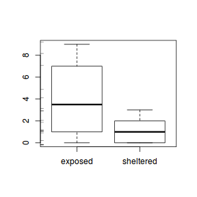
- Compare the expected number of zeros to the actual number of zeros to determine whether the model might be zero inflated.
- Calculate the proportion of zeros in the data
Show code
limpets.tab<-table(limpets$Count==0) limpets.tab/sum(limpets.tab)
FALSE TRUE 0.75 0.25
- Now work out the proportion of zeros we would expect from a Poisson distribution with a lambda equal to the mean count of limpets in this study.
Show codeClearly there are substantially more zeros than expected so the data are likely to be zero inflated.
limpets.mu <- mean(limpets$Count) cnts <-rpois(1000,limpets.mu) limpets.tab<-table(cnts==0) limpets.tab/sum(limpets.tab)
FALSE TRUE 0.91 0.09
- Calculate the proportion of zeros in the data
- Explore the distribution of counts from each population
-
Lets then fit these data via a zero-inflated Poisson (ZIP) model.
Show code
library(pscl) limpets.zip <- zeroinfl(Count~Shore|1, dist="poisson",data=limpets)
- Check the model for lack of fit via:
- Pearson Χ2
Show code
limpets.resid <- sum(resid(limpets.zip, type="pearson")^2) 1-pchisq(limpets.resid, limpets.zip$df.resid)
[1] 0.2810221
#No evidence of a lack of fit
- Pearson Χ2
- Estimate the dispersion parameter to evaluate over dispersion in the fitted model
- Via Pearson residuals
Show code
limpets.resid/limpets.zip$df.resid
[1] 1.168722
#No evidence of over dispersion
- Via Pearson residuals
- Check the model for lack of fit via:
-
We can now test the null hypothesis that there is no effect of shore type on the abundance of scaley limpets;
- Wald z-tests (these are equivalent to t-tests)
- Chisq-test. Note that Chisq = z2
- F-test. Note that Chisq = z2
Show codesummary(limpets.zip)
Call: zeroinfl(formula = Count ~ Shore | 1, data = limpets, dist = "poisson") Pearson residuals: Min 1Q Median 3Q Max -1.54025 -0.93957 -0.04699 0.84560 1.76938 Count model coefficients (poisson with log link): Estimate Std. Error z value Pr(>|z|) (Intercept) 1.6002 0.1619 9.886 < 2e-16 *** Shoresheltered -1.3810 0.3618 -3.817 0.000135 *** Zero-inflation model coefficients (binomial with logit link): Estimate Std. Error z value Pr(>|z|) (Intercept) -1.6995 0.7568 -2.246 0.0247 * --- Signif. codes: 0 '***' 0.001 '**' 0.01 '*' 0.05 '.' 0.1 ' ' 1 Number of iterations in BFGS optimization: 13 Log-likelihood: -37.53 on 3 DfShow codelibrary(car) Anova(limpets.zip,test.statistic="Chisq")
Analysis of Deviance Table (Type II tests) Response: Count Df Chisq Pr(>Chisq) Shore 1 14.57 0.0001351 *** Residuals 17 --- Signif. codes: 0 '***' 0.001 '**' 0.01 '*' 0.05 '.' 0.1 ' ' 1Show codelibrary(car) Anova(limpets.zip,test.statistic="F")
Analysis of Deviance Table (Type II tests) Response: Count Df F Pr(>F) Shore 1 14.57 0.001379 ** Residuals 17 --- Signif. codes: 0 '***' 0.001 '**' 0.01 '*' 0.05 '.' 0.1 ' ' 1
Log-linear modelling
Roberts (1993) was intested in examining the interaction between the presence of dead coolibah trees and the position of quadrats along a transect.
Download Roberts data set
Open the roberts data file (HINT).Format of roberts.csv data file COOLIBAH POSITION COUNT WITH BOTTOM 15 WITH MIDDLE 4 WITH TOP 0 WITHOUT BOTTOM 13 WITHOUT MIDDLE 8 WITHOUT TOP 17 COOLIBAH Categorical listing whether or not dead coolibahs are present (WITH) or absent (WITHOUT) from the quadrat POSITION Position of the quadrat along a transect PA Number of quadrats in each classification
 Show code
roberts <- read.table('../downloads/data/roberts.csv', header=T, sep=',', strip.white=T) head(roberts)
COOLIBAH POSITION COUNT 1 WITH BOTTOM 15 2 WITH MIDDLE 4 3 WITH TOP 0 4 WITHOUT BOTTOM 13 5 WITHOUT MIDDLE 8 6 WITHOUT TOP 17
- Fit a log-linear model to examine the interaction between presence of dead coolibah trees and position along
transect HINT) by first fitting a reduced model (one without the interaction,
HINT),
then fitting the full model (one with the interaction,
HINT)
and finally comparing the reduced model to the full model via analysis of deviance (HINT).
Show codeAlternatively, we can just generate an ANOVA (deviance) table from the full model and ignore the non-interaction terms (HINT).
#Reduced model roberts.glmR <- glm(COUNT ~ POSITION + COOLIBAH, family=poisson, data=roberts) #Full model roberts.glmF <- glm(COUNT ~ POSITION * COOLIBAH, family=poisson, data=roberts) #Compare the two models anova(roberts.glmR,roberts.glmF,test='Chisq')
Analysis of Deviance Table Model 1: COUNT ~ POSITION + COOLIBAH Model 2: COUNT ~ POSITION * COOLIBAH Resid. Df Resid. Dev Df Deviance Pr(>Chi) 1 2 18.613 2 0 0.000 2 18.613 9.083e-05 *** --- Signif. codes: 0 '***' 0.001 '**' 0.01 '*' 0.05 '.' 0.1 ' ' 1
Show codeIdentify the following:anova(roberts.glmF, test="Chisq")
Analysis of Deviance Table Model: poisson, link: log Response: COUNT Terms added sequentially (first to last) Df Deviance Resid. Df Resid. Dev Pr(>Chi) NULL 5 31.974 POSITION 2 6.9044 3 25.069 0.03168 * COOLIBAH 1 6.4562 2 18.613 0.01106 * POSITION:COOLIBAH 2 18.6130 0 0.000 9.083e-05 *** --- Signif. codes: 0 '***' 0.001 '**' 0.01 '*' 0.05 '.' 0.1 ' ' 1
- G2
- df
- P value
- G2
- Perhaps to help provide more insights into the drivers of the significant association between the coolibah mortality and position along the transect,
we could explore the odds ratios. Recall that for logit models, the slope terms are expressed on the log odds-ratio scale and thus
can be simply translated into odds-ratios. That said, again it is only the interaction terms that are of interest.
Nevertheless, as one of the observed counts is 0, the slope terms for any interactions involving this cell will be very large (and the exponent likely to be infinite). One possible remedy is to refit the model after adding a small constant (such as 0.5) to all the observed counts and then calculate the odds ratios.
Show coderoberts.glmF1 <- glm(I(COUNT+0.5) ~ POSITION*COOLIBAH, family=poisson, data=roberts) library(biology) odds.ratio(roberts.glmF1)
Odds ratio Lower 95% CI Upper 95% CI POSITIONMIDDLE 0.29032258 0.101643543 0.8292430 POSITIONTOP 0.03225806 0.001930171 0.5391142 COOLIBAHWITHOUT 0.87096774 0.419874278 1.8066951 POSITIONMIDDLE:COOLIBAHWITHOUT 2.16872428 0.559012753 8.4136989 POSITIONTOP:COOLIBAHWITHOUT 40.18518519 2.201684114 733.4608532
An additional issue that no doubt you noticed is that as the model is fitted as an 'effects' parameterization, not all pairwise calculations are defined. For example, the interaction terms define the (log) odds ratios for with and without coolibah trees in the bottom of the transect versus the middle and versus the top. Hence we only have odds ratios for two of the three comparisons (we don't have middle vs top)
We could derive this other odds ratio by either redefining the model contrasts. Alternatively, we could just calculate the pairwise odds ratios from a cross table representation of the frequency data (again adding a constant of 0.5).
Show codeWhat addition conclusions would you draw?roberts.xtab <- xtabs(COUNT+0.5~POSITION+COOLIBAH, data=roberts) library(biology) oddsratios(roberts.xtab)
Error: could not find function "oddsratio.wald"
#you are 40 times more likely to encounter dead coolibah trees at the bottom of the transect than at the top.
Log-linear modelling
Sinclair investigated the association between sex, health and cause of death in wildebeest. To do so, they recorded the sex and cause of death (predator or not) of wildebeest carcasses along with a classification of a bone marrow sample. The color and consistency of bone marrow is apparently a reasonably good indication of the health status of an animal (even after death).
Download Sinclair data set
Open the sinclair data file (HINT).Format of sinclair.csv data file SEX MARROW DEATH COUNT FEMALE SWF PRED 26 MALE SWF PRED 14 FEMALE OG PRED 32 MALE OG PRED 43 FEMALE TG PRED 8 MALE TG PRED 10 FEMALE SWF NPRED 6 MALE SWF NPRED 7 FEMALE OG NPRED 26 MALE OG NPRED 12 FEMALE TG NPRED 16 MALE TG NPRED 26 
SEX Categorical listing sex of the wildebeast carcasses MARROW Categorical listing of the bone marrow type (SWF: solid white fatty, OG: opaque gelatinous, TG: translucent gelatinous). DEATH Categorical listing of the cause of death (predation or non-predation) COUNT Number of carcasses encountered in each cross-classification. Show codesinclair <- read.table('../downloads/data/sinclair.csv', header=T, sep=',', strip.white=T) head(sinclair)
SEX MARROW DEATH COUNT 1 FEMALE SWF PRED 26 2 MALE SWF PRED 14 3 FEMALE OG PRED 32 4 MALE OG PRED 43 5 FEMALE TG PRED 8 6 MALE TG PRED 10
- What is the null hypothesis of interest?
- Log-linear models for three way tables have a greater number of interactions and therefore a greater number of combinations of terms that should be tested. As with ANOVA, it is the higher level interactions (three way) interaction that is of initial interest, followed by the various two way interactions.
-
Test the null hypothesis that there is no three way interaction (the cause of death is independent of sex and bone marrow type).
First fit a reduced model (one that contains all two way interactions as well as individual effects but without the three way interaction,
HINT),
then fitting the full model (one with the interaction and all other terms,
HINT)
and finally comparing the reduced model to the full model (HINT).
Show codesinclair.glmR <- glm(COUNT~SEX:DEATH + SEX:MARROW + MARROW:DEATH + SEX + DEATH + MARROW, family=poisson,data=sinclair) sinclair.glmF <- glm(COUNT~SEX*DEATH*MARROW, family=poisson,data=sinclair) anova(sinclair.glmR,sinclair.glmF,test='Chisq')
Analysis of Deviance Table Model 1: COUNT ~ SEX:DEATH + SEX:MARROW + MARROW:DEATH + SEX + DEATH + MARROW Model 2: COUNT ~ SEX * DEATH * MARROW Resid. Df Resid. Dev Df Deviance Pr(>Chi) 1 2 7.1883 2 0 0.0000 2 7.1883 0.02748 * --- Signif. codes: 0 '***' 0.001 '**' 0.01 '*' 0.05 '.' 0.1 ' ' 1#OR just anova(sinclair.glmF,test='Chisq')
Analysis of Deviance Table Model: poisson, link: log Response: COUNT Terms added sequentially (first to last) Df Deviance Resid. Df Resid. Dev Pr(>Chi) NULL 11 76.950 SEX 1 0.0177 10 76.932 0.894163 DEATH 1 7.1171 9 69.815 0.007635 ** MARROW 2 27.0529 7 42.763 1.335e-06 *** SEX:DEATH 1 0.0866 6 42.676 0.768531 SEX:MARROW 2 4.7779 4 37.898 0.091725 . DEATH:MARROW 2 30.7097 2 7.188 2.145e-07 *** SEX:DEATH:MARROW 2 7.1883 0 0.000 0.027484 * --- Signif. codes: 0 '***' 0.001 '**' 0.01 '*' 0.05 '.' 0.1 ' ' 1G2 df P SEX:MARROW:DEATH - We would clearly reject the null hypothesis of no three way interaction.
As with ANOVA, following a significant interaction it is necessary to slip the data up according to the levels of one of the factors and explore the
patterns further within the multiple subsets.
- Sinclair and Arcese (1995) might have been interesting in investigating the associations between cause of death and marrow type separately for each sex. Split the sinclair data set up by sex. (HINT)
-
Perform the log-linear modelling for the associations between cause of death and marrow type separately for each sex.
Show code
sinclair.glmR <- glm(COUNT~DEATH+MARROW, family=poisson, data=sinclair.split[["FEMALE"]]) sinclair.glmF <- glm(COUNT~DEATH*MARROW, family=poisson, data=sinclair.split[["FEMALE"]]) anova(sinclair.glmR, sinclair.glmF, test="Chisq")
Analysis of Deviance Table Model 1: COUNT ~ DEATH + MARROW Model 2: COUNT ~ DEATH * MARROW Resid. Df Resid. Dev Df Deviance Pr(>Chi) 1 2 13.963 2 0 0.000 2 13.963 0.0009291 *** --- Signif. codes: 0 '***' 0.001 '**' 0.01 '*' 0.05 '.' 0.1 ' ' 1
#Alternatively, the splitting and subsetting can be performed inline #I shall illustrate this with the MALE data sinclair.glmR <- glm(COUNT~DEATH+MARROW, family=poisson, data=sinclair, subset=sinclair$SEX=="MALE") sinclair.glmF <- glm(COUNT~DEATH*MARROW, family=poisson, data=sinclair, subset=sinclair$SEX=="MALE") anova(sinclair.glmR, sinclair.glmF, test="Chisq")
Analysis of Deviance Table Model 1: COUNT ~ DEATH + MARROW Model 2: COUNT ~ DEATH * MARROW Resid. Df Resid. Dev Df Deviance Pr(>Chi) 1 2 23.935 2 0 0.000 2 23.935 6.346e-06 *** --- Signif. codes: 0 '***' 0.001 '**' 0.01 '*' 0.05 '.' 0.1 ' ' 1
Show codesinclair.split <- split(sinclair, sinclair$SEX) sinclair.split
$FEMALE SEX MARROW DEATH COUNT 1 FEMALE SWF PRED 26 3 FEMALE OG PRED 32 5 FEMALE TG PRED 8 7 FEMALE SWF NPRED 6 9 FEMALE OG NPRED 26 11 FEMALE TG NPRED 16 $MALE SEX MARROW DEATH COUNT 2 MALE SWF PRED 14 4 MALE OG PRED 43 6 MALE TG PRED 10 8 MALE SWF NPRED 7 10 MALE OG NPRED 12 12 MALE TG NPRED 26G2 df P Females - MARROW:DEATH Males - MARROW:DEATH -
It appears that there are significant interactions between cause of death and bone marrow type for both females and males.
Given that there was a significant interaction between cause of death and sex and bone marrow type, it is likely that the nature of the two way interactions in females is different to the two way interactions in males.
To explore this further, we will examine the odds ratios for each pairwise comparison of bone marrow type with respect to predation level (for each sex)!.
Calculate the odds ratios for wildebeest killed by predation for each pair of marrow types separately for males and females .
Show codelibrary(epitools)
Error in library(epitools): there is no package called 'epitools'
library(biology) #Females female.tab <- xtabs(COUNT ~ DEATH + MARROW, data=sinclair.split[["FEMALE"]]) female.odds<-oddsratios(t(female.tab))
Error: could not find function "oddsratio.wald"
female.oddsError in eval(expr, envir, enclos): object 'female.odds' not found
#Males male.tab <- xtabs(COUNT ~ DEATH + MARROW, data=sinclair.split[["MALE"]]) male.odds<-oddsratios(t(male.tab))
Error: could not find function "oddsratio.wald"
Odds ratio 95% CI min 95% CI max Females OG vs TG SWF vs TG SWF vs OG Males OG vs TG SWF vs TG SWF vs OG -
The patterns revealed in the odds ratios might be easier to see, if they were presented graphically - do it.
Show code
par(mar=c(5,5,0,0)) plot(estimate~as.numeric(Comparison), data=female.odds, log="y", type="n", axes=F, ann=F, ylim=range(c(upper,lower)), xlim=c(0.5,3.5))
Error in eval(expr, envir, enclos): object 'female.odds' not found
with(female.odds,arrows(as.numeric(Comparison)+0.1,upper,as.numeric(Comparison)+0.1,lower,ang=90,length=0.1,code=3))
Error in with(female.odds, arrows(as.numeric(Comparison) + 0.1, upper, : object 'female.odds' not found
with(female.odds,points(as.numeric(Comparison)+0.1,estimate, type="b", pch=21, bg="white"))
Error in with(female.odds, points(as.numeric(Comparison) + 0.1, estimate, : object 'female.odds' not found
#males with(male.odds,arrows(as.numeric(Comparison)-0.1,upper,as.numeric(Comparison)-0.1,lower,ang=90,length=0.1,code=3))
Error in with(male.odds, arrows(as.numeric(Comparison) - 0.1, upper, as.numeric(Comparison) - : object 'male.odds' not found
with(male.odds,points(as.numeric(Comparison)-0.1,estimate, type="b", pch=21, bg="black",lty=1))
Error in with(male.odds, points(as.numeric(Comparison) - 0.1, estimate, : object 'male.odds' not found
abline(h=1,lty=2)
Error in int_abline(a = a, b = b, h = h, v = v, untf = untf, ...): plot.new has not been called yet
with(female.odds, axis(1,at=as.numeric(Comparison), lab=Comparison))
Error in with(female.odds, axis(1, at = as.numeric(Comparison), lab = Comparison)): object 'female.odds' not found
mtext("Marrow type",1,line=3, cex=1.25)
Error in mtext("Marrow type", 1, line = 3, cex = 1.25): plot.new has not been called yetaxis(2,las=1)
Error in axis(2, las = 1): plot.new has not been called yet
mtext("Odds ratio of death by predation",2,line=4, cex=1.25)
Error in mtext("Odds ratio of death by predation", 2, line = 4, cex = 1.25): plot.new has not been called yetlegend("topright",legend=c("Male","Female"),pch=21, bty="n", title="Sex",pt.bg=c("black","white"))
Error in strwidth(legend, units = "user", cex = cex, font = text.font): plot.new has not been called yet
box(bty="l")
Error in box(bty = "l"): plot.new has not been called yet
- What would your conclusions be?
- Check the model for lack of fit via:
Conclusions - the relationship between fitted values and observed counts is reasonable without being spectacular.
Exploring the model parameters, test hypotheses
If there was any evidence that the assumptions had been violated or the model was not an appropriate fit, then we would need to reconsider the model and start the process again. In this case, there is no evidence that the test will be unreliable so we can proceed to explore the test statistics. The main statistic of interest is the Wald statistic ($z$) for the zeroinfl model and the t-statistic ($t$) for the gamlss model. The analyses are partitioned into the binary and Poisson components. For the Poisson component, it is the slope parameter that is of the primary interest. Since the models specified that the binomial component was to be modeled only against an intercept, the binomial output includes only an estimate for the intercept.
Conclusions: We would reject the null hypothesis (p<0.05) from each model. Note that the two different approaches adopt a differnet reference distribution. Whilst zeroinf uses the Wald statistic ($z$), gamlss uses the t-statistic ($t$). An increase in x is associated with a significant linear increase (positive slope) in log $y$ abundance. Every 1 unit increase in $x$ is associated with a 0.087 unit increase in $\log y$ abundance We usually express this in terms of $y$ than $\log y$, so every 1 unit increase in $x$ is associated with a ($e^{0.087}=1.09$) 1.09 unit increase in $y$ abundance.
Further explorations of the trends
Now for a summary plot.
par(mar = c(4, 5, 0, 0))
plot(y ~ x, data = dat.zip, type = "n", ann = F, axes = F)
points(y ~ x, data = dat.zip, pch = 16)
xs <- seq(min(dat.zip$x), max(dat.zip$x), l=100)
coefs <- coef(dat.zeroinfl, model="count")
mm <- model.matrix(~x, data=data.frame(x=xs))
vcov <- vcov(dat.zeroinfl, model="count")
ys <- vector("list")
ys$fit <- exp(mm %*% coefs)
points(ys$fit ~ xs, col = "black", type = "l")

ys$se.fit <- exp(sqrt(diag(mm %*% vcov %*% t(mm))))
lines(ys$fit - 1 * ys$se.fit ~ xs, col = "black", type = "l", lty = 2)
lines(ys$fit + 1 * ys$se.fit ~ xs, col = "black", type = "l", lty = 2)
axis(1)
mtext("X", 1, cex = 1.5, line = 3)
axis(2, las = 2)
mtext("Abundance of Y", 2, cex = 1.5, line = 3)
box(bty = "l")
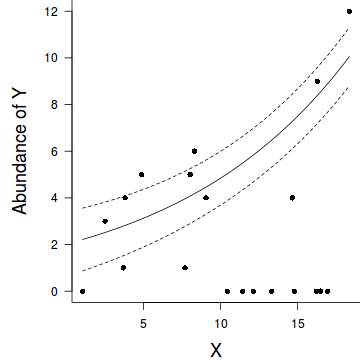
Log-linear models
Scenario and Data
Worked Examples
Basic χ2 references
Poisson t-test
A marine ecologist was interested in examining the effects of wave exposure on the abundance of the striped limpet Siphonaria diemenensis on rocky intertidal shores. To do so, a single quadrat was placed on 10 exposed (to large waves) shores and 10 sheltered shores. From each quadrat, the number of Siphonaria diemenensis were counted.
Download Limpets data setFormat of limpets.csv data files Count Shore 1 sheltered 3 sheltered 2 sheltered 1 sheltered 4 sheltered ... ... Shore Categorical description of the shore type (sheltered or exposed) - Predictor variable Count Number of limpets per quadrat - Response variable 
Open the limpet data set.
Show codelimpets <- read.table('../downloads/data/limpets.csv', header=T, sep=',', strip.white=T) limpets
   Count     Shore
1      2 sheltered
2      2 sheltered
3      0 sheltered
4      6 sheltered
5      0 sheltered
6      3 sheltered
7      3 sheltered
8      0 sheltered
9      1 sheltered
10     2 sheltered
11     5   exposed
12     3   exposed
13     6   exposed
14     3   exposed
15     4   exposed
16     7   exposed
17    10   exposed
18     3   exposed
19     5   exposed
20     2   exposed
The design is clearly a t-test as we are interested in comparing two population means (mean number of striped limpets on exposed and sheltered shores). Recall that a parametric t-test assumes that the residuals (and populations from which the samples are drawn) are normally distributed and equally varied.
At this point we could transform the data in an attempt to satisfy normality and homogeneity of variance. However, the analyses are then not on the scale of the data and thus the conclusions also pertain to a different scale. Furthermore, linear modelling on transformed count data is generally not as effective as modelling count data with a Poisson distribution.
Poisson ANOVA (regression)
We once again return to a modified example from Quinn and Keough (2002). In Exercise 1 of Workshop 9.4a, we introduced an experiment by Day and Quinn (1989) that examined how rock surface type affected the recruitment of barnacles to a rocky shore. The experiment had a single factor, surface type, with 4 treatments or levels: algal species 1 (ALG1), algal species 2 (ALG2), naturally bare surfaces (NB) and artificially scraped bare surfaces (S). There were 5 replicate plots for each surface type and the response (dependent) variable was the number of newly recruited barnacles on each plot after 4 weeks.
Download Day data set
Open the day data file.Format of day.csv data files TREAT BARNACLE ALG1 27 .. .. ALG2 24 .. .. NB 9 .. .. S 12 .. .. TREAT Categorical listing of surface types. ALG1 = algal species 1, ALG2 = algal species 2, NB = naturally bare surface, S = scraped bare surface. BARNACLE The number of newly recruited barnacles on each plot after 4 weeks.  Show code
day <- read.table('../downloads/data/day.csv', header=T, sep=',', strip.white=T)
head(day)
  TREAT BARNACLE
1  ALG1       27
2  ALG1       19
3  ALG1       18
4  ALG1       23
5  ALG1       25
6  ALG2       24
We previously analysed these data with via a classic linear model (ANOVA) as the data appeared to conform to the linear model assumptions. Alternatively, we could analyse these data with a generalized linear model (Poisson error distribution). Note that as the boxplots were all fairly symmetrical and equally varied, and the sample means are well away from zero (in fact there are no zero's in the data) we might suspect that whether we fit the model as a linear or generalized linear model is probably not going to be of great consequence. Nevertheless, it does then provide a good comparison between the two frameworks.
Poisson ANOVA (regression)
To investigate habitat differences in moth abundances, researchers from the Australian National University (ANU) in Canberra counted the number of individuals of two species of moth (recorded as A and P) along transects throughout a landscape comprising eight different habitat types ('Bank', 'Disturbed', 'Lowerside', 'NEsoak', 'NWsoak', 'SEsoak', 'SWsoak', 'Upperside'). For the data presented here, one of the habitat types ('Bank') has been ommitted as no moths were encounted in that habitat.
Although each transect was approximately the same length, each transect passed through multiple habitat types. Consequently, each transect was divided into sections according to habitat and the number of moths observed in each section recorded. Clearly, the number of observed moths in a section would be related to the length of the transect in that section. Therefore, the researchers also recorded the length of each habitat section.
Download moths data set
Open the day data file.Format of moth.csv data files METERS A P HABITAT 25 9 8 NWsoak 37 3 20 SWsoak 109 7 9 Lowerside 10 0 2 Lowerside 133 9 1 Upperside 26 3 18 Disturbed METERS The length of the section of transect A The number of moth species A observed in section of transect P The number of moth species P observed in section of transect HABITAT Categorical listing of the habitat type within section of transect.  Show code
moths <- read.csv('../downloads/data/moths.csv', header=T, strip.white=T) head(moths)
METERS A P HABITAT 1 25 9 8 NWsoak 2 37 3 20 SWsoak 3 109 7 9 Lowerside 4 10 0 2 Lowerside 5 133 9 1 Upperside 6 26 3 18 Disturbed
The primary focus of this question will be to investigate the effect of habitat on the abundance of moth species A.
- Deviance ($G^2$) - similar to the $\chi^2$ test above, yet uses deviance
