Tutorial 14.3 - Correspondance Analysis (CA)
11 Jun 2015
> library(vegan)
> library(ggplot2)
> library(grid)
> #define my common ggplot options
> murray_opts <- opts(panel.grid.major=theme_blank(),
+                            panel.grid.minor=theme_blank(),
+                            panel.border = theme_blank(),
+                            panel.background = theme_blank(),
+                            axis.title.y=theme_text(size=15, vjust=0,angle=90),
+                            axis.text.y=theme_text(size=12),
+                            axis.title.x=theme_text(size=15, vjust=-1),
+                            axis.text.x=theme_text(size=12),
+                            axis.line = theme_segment(),
+                            plot.margin=unit(c(0.5,0.5,1,2),"lines")
+ )
Error: Use 'theme' instead. (Defunct; last used in version 0.9.1)
> coenocline <- function(x,A0,m,r,a,g, int=T, noise=T) {
+ #x is the environmental range
+ #A0 is the maximum abundance of the species at the optimum environmental conditions
+ #m is the value of the environmental gradient that represents the optimum conditions for the species
+ #r the species range over the environmental gradient (niche width)
+ #a and g are shape parameters representing the skewness and kurtosis
+ # when a=g, the distribution is symmetrical
+ # when a>g - negative skew (large left tail)
+ # when a<g - positive skew (large right tail)
+ #int - indicates whether the responses should be rounded to integers (=T)
+ #noise - indicates whether or not random noise should be added (reflecting random sampling)
+ #NOTE.  negative numbers converted to 0
+          b <- a/(a+g)
+          d <- (b^a)*(1-b)^g
+          cc <- (A0/d)*((((x-m)/r)+b)^a)*((1-(((x-m)/r)+b))^g)
+          if (noise) {n <- A0/10; n[n<0]<-0; cc<-cc+rnorm(length(cc),0,n)}
+          cc[cc<0] <- 0
+          cc[is.na(cc)]<-0
+          if (int) cc<-round(cc,0)
+          cc
+ }
> #plot(coenocline(0:100,40,40,20,1,1, int=T, noise=T), ylim=c(0,100))
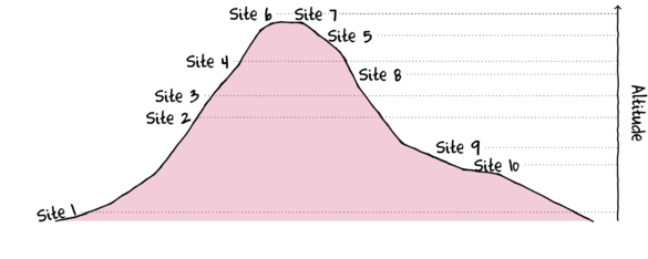
To assist with demonstrating Correspondence Analysis (CA), we will return to the fabricated species abundance data introduced at the start of Tutorial 14.2. This data set comprises the abundances of 10 species within 10 sites located along a transect that extends in a northerly direction over a mountain range.

> set.seed(1)
> x <- seq(0,50,l=10)
> n <- 10
> sp1<-coenocline(x=x,A0=5,m=0,r=2,a=1,g=1,int=T, noise=T)
> sp2<-coenocline(x=x,A0=70,m=7,r=30,a=1,g=1,int=T, noise=T)
> sp3<-coenocline(x=x,A0=50,m=15,r=30,a=1,g=1,int=T, noise=T)
> sp4<-coenocline(x=x,A0=7,m=25,r=20,a=0.4,g=0.1,int=T, noise=T)
> sp5<-coenocline(x=x,A0=40,m=30,r=30,a=0.6,g=0.5,int=T, noise=T)
> sp6<-coenocline(x=x,A0=15,m=35,r=15,a=0.2,g=0.3,int=T, noise=T)
> sp7<-coenocline(x=x,A0=20,m=45,r=25,a=0.5,g=0.9,int=T, noise=T)
> sp8<-coenocline(x=x,A0=5,m=45,r=5,a=1,g=1,int=T, noise=T)
> sp9<-coenocline(x=x,A0=20,m=45,r=15,a=1,g=1,int=T, noise=T)
> sp10<-coenocline(x=x,A0=30,m=50,r=5,a=1,g=1,int=T, noise=T)
> X <- cbind(sp1, sp10,sp9,sp2,sp3,sp8,sp4,sp5,sp7,sp6)
> #X<-X[c(1,10,9,2,3,8,4,5,7,6),]
> colnames(X) <- paste("Sp",1:10,sep="")
> rownames(X) <- paste("Site", c(1,10,9,2,3,8,4,5,7,6), sep="")
> X <- X[c(1,4,5,7,8,10,9,6,3,2),]
> data <- data.frame(Sites=factor(rownames(X),levels=rownames(X)), X)
| Sites | Sp1 | Sp2 | Sp3 | Sp4 | Sp5 | Sp6 | Sp7 | Sp8 | Sp9 | Sp10 | |
|---|---|---|---|---|---|---|---|---|---|---|---|
| Site1 | Site1 | 5 | 0 | 0 | 65 | 5 | 0 | 0 | 0 | 0 | 0 |
| Site2 | Site2 | 0 | 0 | 0 | 25 | 39 | 0 | 6 | 23 | 0 | 0 |
| Site3 | Site3 | 0 | 0 | 0 | 6 | 42 | 0 | 6 | 31 | 0 | 0 |
| Site4 | Site4 | 0 | 0 | 0 | 0 | 0 | 0 | 0 | 40 | 0 | 14 |
| Site5 | Site5 | 0 | 0 | 6 | 0 | 0 | 0 | 0 | 34 | 18 | 12 |
| Site6 | Site6 | 0 | 29 | 12 | 0 | 0 | 0 | 0 | 0 | 22 | 0 |
| Site7 | Site7 | 0 | 0 | 21 | 0 | 0 | 5 | 0 | 0 | 20 | 0 |
| Site8 | Site8 | 0 | 0 | 0 | 0 | 13 | 0 | 6 | 37 | 0 | 0 |
| Site9 | Site9 | 0 | 0 | 0 | 60 | 47 | 0 | 4 | 0 | 0 | 0 |
| Site10 | Site10 | 0 | 0 | 0 | 72 | 34 | 0 | 0 | 0 | 0 | 0 |
Tutorial 14.2 demonstrated the the susceptibility of Principle Components Analysis (PCA) to the horseshoe or arch effect when applied to species abundance data. In a PCA, objects (sites) are projected onto what is essentially a rotated variable (species) space. That is, the original axes represent the variables (species). The rotated axes are just a re-expression of these axes. The PCA therefore assumes multivariate linearity. By extension, the species response curves are also assumed to be linear with respect to any underlying gradients.
This is a somewhat unrealistic expectation for species abundance curves, particularly if the study occurs at a reasonably large spatial scale (which is often the case).
By contrast, Correspondence Analysis (CA) projects objects (sites) and variables (species) into a new ordination space (that theoretically represents the major underlying environmental gradients). Rather than base associations on a covariance or correlation matrix (from which axes rotation maintains the euclidean distances between objects), in CA, single value decomposition is performed on a matrix of $\chi^2$ contributions (standardized $\chi^2$ residuals) and therefore preserves $\chi^2$ distances between objects (sites).
The data (typically species abundance or presence/absence data) must be frequencies and are assumed to be unimodal with respect to the underlying gradients (which suits species abundance data nicely). Frequencies are calculated by dividing each value by its column (species) total.
> #convert to frequencies (of row and columns)
> # MARGIN=2 indicates columns
> data <- decostand(data[,-1],method="total",MARGIN=2)
> data
       Sp1 Sp2       Sp3        Sp4
Site1    1   0 0.0000000 0.28508772
Site2    0   0 0.0000000 0.10964912
Site3    0   0 0.0000000 0.02631579
Site4    0   0 0.0000000 0.00000000
Site5    0   0 0.1538462 0.00000000
Site6    0   1 0.3076923 0.00000000
Site7    0   0 0.5384615 0.00000000
Site8    0   0 0.0000000 0.00000000
Site9    0   0 0.0000000 0.26315789
Site10   0   0 0.0000000 0.31578947
              Sp5 Sp6       Sp7
Site1  0.02777778   0 0.0000000
Site2  0.21666667   0 0.2727273
Site3  0.23333333   0 0.2727273
Site4  0.00000000   0 0.0000000
Site5  0.00000000   0 0.0000000
Site6  0.00000000   0 0.0000000
Site7  0.00000000   1 0.0000000
Site8  0.07222222   0 0.2727273
Site9  0.26111111   0 0.1818182
Site10 0.18888889   0 0.0000000
             Sp8       Sp9      Sp10
Site1  0.0000000 0.0000000 0.0000000
Site2  0.1393939 0.0000000 0.0000000
Site3  0.1878788 0.0000000 0.0000000
Site4  0.2424242 0.0000000 0.5384615
Site5  0.2060606 0.3000000 0.4615385
Site6  0.0000000 0.3666667 0.0000000
Site7  0.0000000 0.3333333 0.0000000
Site8  0.2242424 0.0000000 0.0000000
Site9  0.0000000 0.0000000 0.0000000
Site10 0.0000000 0.0000000 0.0000000
At this point, we could examine a tile plot that represents the relative abundance of each species within each site.

> data.1 <- data.frame(Sites=factor(rownames(data),levels=rownames(data)),data)
> library(reshape)
> data1 <- melt(data.1,id="Sites", variable_name="Species")
> data.xtab <- xtabs(value~Sites+Species, data1)
> library(vcd)
> tile(data.xtab, tile_type="height", shade=F)
If there are any strong underlying environmental gradients (traversed by the sites), then we might expect there to be corresponding
patterns in which certain species are associated with certain sites.
Moreover, since the species response curves (across an environmental gradient)
are expected to be unimodal, then we might expect that the species abundances would be
unimodally distributed across a number of sites.

The above theoretical situation shows a clear association between species abundance and sites - note the diagonal trend from top left to bottom right.
Therefore, if there are strong underlying environmental gradients, we would expect the species and site cross tabulated frequencies to be correlated. And such correlations should occur for each of the major environmental gradients.
Calculating site and species scores
A process of iterative re-weighting is used to calculate the new object (site) and variable (species) scores for each of the new correspondence axes from the matrix of standardized residuals ($\chi^2$ components).
If we the reorder the rows (sites) and columns (species) of the proportional frequency data according to the resulting new site scores and species scores for the first two correspondence axes, we can visualize the result of the iterative re-weighting process.
| Correspondence axis 1 | Correspondence axis 2 |
|---|---|
 |
 |
> data.ca <- cca(data)
> data.cs <- data.ca$CA$u[,1]
> data.rs <- data.ca$CA$v[,1]
> data3 <- data[order(data.cs),order(data.rs)]
>
> data3 <- data.frame(Sites=rownames(data3),data3)
> data4 <- melt(data3,id="Sites", variable_name="Species")
> data4$Sites <- factor(data4$Sites, levels=unique(data4$Sites))
> data4 <- xtabs(value~Sites+Species, data4)
> #tile(data4, tile_type="height", shade=F)
> tile(data4, tile_type="area", halign="center",valign="center",shade=F)
>
> #p <- ggplot(data1,aes(y=value,x=as.numeric(Sites)), group=variable)+geom_ribbon(aes(ymin=0,ymax=value,fill=variable,col=variable), alpha=0.1)
> #p
> data.cs <- data.ca$CA$u[,2]
> data.rs <- data.ca$CA$v[,2]
> data3 <- data[order(data.cs),order(data.rs)]
>
> data3 <- data.frame(Sites=rownames(data3),data3)
> data4 <- melt(data3,id="Sites", variable_name="Species")
> data4$Sites <- factor(data4$Sites, levels=unique(data4$Sites))
> data4 <- xtabs(value~Sites+Species, data4)
> #tile(data4, tile_type="height", shade=F)
> tile(data4, tile_type="area", halign="center",valign="center",shade=F)
- the table rows and columns have been re-ordered to maximize the correlation (correspondence - hence the name) between the objects (sites) and variables (species). This vaguely resembles the theoretical response curves with the diagonal correlation pattern we considered earlier.
- the correspondence (correlation) is higher for the first correspondence axis than the second correspondence axis. The first axis is always the strongest and each additional axis picks up patterns that were missed from earlier axes.
The end result of this process is that since the site and species scores are directed by weighted averages of each other, both objects (sites) and variables (species) are projected in the same ordination space.
Objects and variables are projected in ordination space in the location they are most frequent (corresponding $\chi^2$ are highest). Thus, object (site) and variable (species) scores represent the one configuration (arrangement of sites and species) in which they are maximally correlated.
The eigenvalues resulting from the decomposition measure the degree of correlation between the site and species scores per correspondence axis. That is, the represent how well the species and site scores correspond for that theoretical environmental gradient.
As just stated, both objects (sites) and variables (species) are projected onto the one ordination space. How they are interpreted depends on how they are scaled relative to one another.
- when scaled relative to the variables (species), each variable (species) is projected into the ordination space in the location in which it is most frequent (where it has the highest $\chi^2$ value). Objects (sites) located on the ordination in close proximity to one or more species are likely to be have a substantial abundance of those species.
- when scaled relative to the objects (sites), Species located close by one another are likely to have similar relative frequencies. Species located close to sites are more likely to be found in those sites.
cca()
In R, Correspondance Analysis (CA) is implemented in the cca() function (from the vegan package).
Lets perform a correspondence analysis on the species abundance data. As the first step performed in a correspondence analysis is to transform the abundances into a $\chi^2$ matrix (by weighting the observed frequencies against expected frequencies using the row, column and grand totals), we need to make sure there are no columns or rows that sum to 0. In this particular data set, the condition is met.
We can now perform the correspondence analysis. We will then summarize it scaling the sites proportional to the eignvalues (objects not scaled). We will then scale the objects proportional to the eigenvalues.
> data.ca <- cca(data)
> summary(data.ca)
Call:
cca(X = data)

Partitioning of mean squared contingency coefficient:
              Inertia Proportion
Total           3.256          1
Unconstrained   3.256          1

Eigenvalues, and their contribution to the mean squared contingency coefficient

Importance of components:
                         CA1    CA2
Eigenvalue            0.9463 0.7823
Proportion Explained  0.2906 0.2402
Cumulative Proportion 0.2906 0.5309
                         CA3    CA4
Eigenvalue            0.6214 0.5784
Proportion Explained  0.1908 0.1776
Cumulative Proportion 0.7217 0.8994
                          CA5     CA6
Eigenvalue            0.26286 0.04315
Proportion Explained  0.08073 0.01325
Cumulative Proportion 0.98009 0.99334
                          CA7      CA8
Eigenvalue            0.01551 0.006164
Proportion Explained  0.00476 0.001890
Cumulative Proportion 0.99811 1.000000

Scaling 2 for species and site scores
* Species are scaled proportional to eigenvalues
* Sites are unscaled: weighted dispersion equal on all dimensions


Species scores

         CA1     CA2      CA3      CA4
Sp1  -1.4446  1.8842 -0.86530  0.03061
Sp2   1.1313  0.5380  0.52836  1.74914
Sp3   1.0302  0.3407  0.16160 -0.32148
Sp4  -1.1395  0.2409  0.47543 -0.02254
Sp5  -0.9094 -0.6375  0.85632 -0.03372
Sp6   1.1250  0.5162  0.37542 -1.61102
Sp7  -0.7780 -0.9688  0.78276 -0.02684
Sp8  -0.2565 -1.0628 -0.43367  0.02821
Sp9   0.9388  0.1688 -0.07722  0.11955
Sp10  0.3026 -1.0196 -1.80371  0.08808
          CA5       CA6
Sp1  -0.47720 -0.006432
Sp2  -0.05360  0.247953
Sp3   0.00978 -0.135905
Sp4   1.06125  0.022650
Sp5   0.35896 -0.014035
Sp6  -0.05869  0.265755
Sp7  -0.79494 -0.033065
Sp8  -0.55703  0.053469
Sp9   0.07364 -0.513328
Sp10  0.43783  0.112936


Site scores (weighted averages of species scores)

           CA1     CA2     CA3      CA4
Site1  -1.4446  1.8842 -0.8653  0.03061
Site2  -0.8156 -0.9072  0.8514 -0.03082
Site3  -0.7373 -1.0761  0.7693 -0.02515
Site4   0.1364 -1.3205 -2.2180  0.12014
Site5   0.4965 -0.6686 -1.3203  0.05068
Site6   1.1313  0.5380  0.5284  1.74914
Site7   1.1250  0.5162  0.3754 -1.61102
Site8  -0.6227 -1.2320  0.5034 -0.01041
Site9  -1.0159 -0.5055  1.1190 -0.04803
Site10 -1.1131 -0.1123  0.9944 -0.04620
            CA5       CA6
Site1  -0.47720 -0.006432
Site2  -0.51678 -0.066579
Site3  -1.10800 -0.053106
Site4   0.49068  2.189249
Site5   0.37618 -2.309429
Site6  -0.05360  0.247953
Site7  -0.05869  0.265755
Site8  -2.11065  0.079747
Site9   1.23098 -0.121948
Site10  3.03739  0.206699
Lets go through the output
- Partitioning of mean squared contingency coefficient reaffirms that the analysis is based on the standardized $\chi^2$ residuals.
- inertia in correspondence analysis is the $\chi^2$ value (i.e. the squared sum of the standardized residuals).
- eigenvalues are the degree of correlation between the sites and species for each of the new correspondence axes
and thus a measure of the importance of each axis. The sum of the eigenvalues is the innertia.
Eigenvalues can range from 0 to 1, where an eigenvalue of 1 would indicate that each site has a unique species.
For ecological data, eigenvalues over 0.6 are considered suggesting of a very strong environmental gradient.
In this case, the first three axis have eigenvalues of
0.95,0.78and0.62and thus each would be considered to represent important environmental gradients.The eigenvalues are also expressed as proportions of the total amount explained. These proportions are calculated as the eigenvalues divided by the innertia (as a measure of the total standardized differences between the observed and expected values in the frequency data). In this case, the first three axes explain
29.06%, 24.03%, 19.09%. - scaling refers to the way either objects (sites) or variables (species) are scaled so that
they can both be sensibly included on a biplot.
- scaling=2 (this output) the species scores are scaled proportional to the eigenvalues and sites are unscaled.
This is a good option if the main focus is to interpret the relationships amongst variables (species).
- Species whose points are close together are likely to have similar patterns of frequencies across the sites.
- Species whose points are close to a point representing a site are more likely to be most abundant in that site
- scaling=1 (not in this output) the site scores are scaled proportional to the eigenvalues and species are unscaled.
This is a good option if the main focus is to interpret the relationships amongst objects (sites).
- Sites whose points are close together are likely to have similar patterns of relative species abundances.
- Sites whose points are close to a point representing a species are more likely to contain a relatively high abundance of that species.
- scaling=2 (this output) the species scores are scaled proportional to the eigenvalues and sites are unscaled.
This is a good option if the main focus is to interpret the relationships amongst variables (species).
- species scores these are the (scaled) weighted averages of the site scores.
- site scores these are the (scaled) weighted averages of the species scores. Scores that are close to the origin (0,0) are those with observed frequencies close to the expected frequencies (low standardized residuals).
Axis retention
Determining the number of axes to retain follows the following 'rules':
- eigenvalues greater than the average.
This would suggest that we should consider retaining the first 4 correspondence axes.
> data.ca$CA$eig
        CA1         CA2         CA3
0.946305134 0.782293787 0.621442179
        CA4         CA5         CA6
0.578436060 0.262857400 0.043153975
        CA7         CA8
0.015510825 0.006164366
> mean(data.ca$CA$eig)
[1] 0.4070205
> data.ca$CA$eig>mean(data.ca$CA$eig)
  CA1   CA2   CA3   CA4   CA5   CA6
 TRUE  TRUE  TRUE  TRUE FALSE FALSE
  CA7   CA8
FALSE FALSE
- eigenvalues greater than 0.6 as this is a level representing a strong environmental gradient.
This would suggest that we should consider retaining the first 3 correspondence axes.
> data.ca$CA$eig
        CA1         CA2         CA3
0.946305134 0.782293787 0.621442179
        CA4         CA5         CA6
0.578436060 0.262857400 0.043153975
        CA7         CA8
0.015510825 0.006164366
> data.ca$CA$eig>0.6
  CA1   CA2   CA3   CA4   CA5   CA6
 TRUE  TRUE  TRUE FALSE FALSE FALSE
  CA7   CA8
FALSE FALSE
- an elbow in the screeplot
This would suggest either the first two axes or the first 4 axes.
> screeplot(data.ca)

Ordination plot
An ordination plot including both objects (sites) and variables (species) can be produced with the plot() function
 |
 |
> plot(data.ca, scaling = 1, main = "Scaling=1") > plot(data.ca, scaling=2, main="Scaling=2") |
|
- Species 1 and Site 1 are relatively remote from the other points. This implies that the community at Site 1 was quite different to the other sites. Indeed if we look at the raw data we can see that Site 1 contained three species (Sp1, Sp2 and Sp3) and the former species was only found in Site 1.
- If we just traverse correspondence axis 1 (x-axis), the values range from 1,10,9,2...to 5 and then Sites 6 and 7 are
very close to one another. Reexamining the plot of the study region, axis 1 seems to correspond very well to altitude.
It is likely therefore that the community patterns are related to altitude effects.
- On the second correspondence axis (y-axis), there are a clump of sites (4,8,3,2) low down and at the other extreme there is 6,7 and 1. This is of course fabricated data, yet perhaps that axes relates to temperature where temperatures at the very top and bottom are colder than they are in the middle of the mountain?
- Another important feature is the curved arrangement of points. This is called the arch effect. It is similar to the horseshoe effect that plagues PCA. The arch effect is caused by non-linear relationships between species abundances (similar to the horseshoe effect in PCA), yet unlike the horseshoe effect, the ends do not curl in on themselves. The arch (when present) is typically very sharp with what appears to be two different trends joined at the tip.
I will also introduce another simulated data set that comprises five biophysical measurements made from the 10 sites. These biophysical environmental data include pH (log scale), Pressure (Pa), Altitude (m), Slope (degrees) and Substrate (categorical: Quartz or Shale).
> set.seed(1)
> Site <- gl(10,1,10,lab=paste('Site',1:10, sep=""))
> Y <- matrix(c(
+ 6.1,4.2,101325,2,
+ 6.7,9.2,101352,510,
+ 6.8,8.6,101356,546,
+ 7.0,7.4,101372,758,
+ 7.2,5.8,101384,813,
+ 7.5,8.4,101395,856,
+ 7.5,0.5,101396,854,
+ 7.0,11.8,101370,734,
+ 8.4,8.2,101347,360,
+ 6.2,1.5,101345,356
+   ),10,4, byrow=TRUE)
> colnames(Y) <- c('pH','Slope', 'Pressure', 'Altitude')
> Substrate <- factor(c('Quartz','Shale','Shale','Shale','Shale','Quartz','Quartz','Shale','Quartz','Quartz'))
> enviro <- data.frame(Site,Y,Substrate)
| Site | pH | Slope | Pressure | Altitude | Substrate |
|---|---|---|---|---|---|
| Site1 | 6.1 | 4.2 | 101325 | 2 | Quartz |
| Site2 | 6.7 | 9.2 | 101352 | 510 | Shale |
| Site3 | 6.8 | 8.6 | 101356 | 546 | Shale |
| Site4 | 7.0 | 7.4 | 101372 | 758 | Shale |
| Site5 | 7.2 | 5.8 | 101384 | 813 | Shale |
| Site6 | 7.5 | 8.4 | 101395 | 856 | Quartz |
| Site7 | 7.5 | 0.5 | 101396 | 854 | Quartz |
| Site8 | 7.0 | 11.8 | 101370 | 734 | Shale |
| Site9 | 8.4 | 8.2 | 101347 | 360 | Quartz |
| Site10 | 6.2 | 1.5 | 101345 | 356 | Quartz |
> envfit(data.ca,env=enviro[,-1])
***VECTORS

              CA1      CA2     r2
pH        0.91731 -0.39818 0.4044
Slope    -0.41261 -0.91091 0.3135
Pressure  0.98437 -0.17609 0.9833
Altitude  0.90763 -0.41978 0.9828
         Pr(>r)
pH        0.245
Slope     0.365
Pressure  0.001 ***
Altitude  0.001 ***
---
Signif. codes:
  0 '***' 0.001 '**' 0.01 '*' 0.05
  '.' 0.1 ' ' 1
P values based on 999 permutations.

***FACTORS:

Centroids:
                    CA1     CA2
SubstrateQuartz  0.1358  0.6470
SubstrateShale  -0.2098 -0.9992

Goodness of fit:
              r2 Pr(>r)
Substrate 0.3375  0.065 .
---
Signif. codes:
  0 '***' 0.001 '**' 0.01 '*' 0.05
  '.' 0.1 ' ' 1
P values based on 999 permutations.
> plot(data.ca)
> plot(envfit(data.ca,env=enviro[,-1]))

Now lets regress the first three principle components (individually) against a couple of these environmental predictions (altitude, temperature and slope).
> library(car)
> vif(lm(data.ca$CA$u[,1]~Altitude+Slope+pH+Substrate, data=enviro))
 Altitude     Slope        pH Substrate
 1.830014  2.116732  1.968157  2.636302
> data.lm <- lm(data.ca$CA$u[,1:3] ~ enviro$Altitude + enviro$Slope+enviro$pH+enviro$Substrate)
> summary(data.lm)
Response CA1 :

Call:
lm(formula = CA1 ~ enviro$Altitude + enviro$Slope + enviro$pH +
    enviro$Substrate)

Residuals:
    Site1     Site2     Site3     Site4
 0.422144  0.061252 -0.002323  0.112485
    Site5     Site6     Site7     Site8
 0.232025  0.287221 -0.002549 -0.403439
    Site9    Site10
-0.161979 -0.544838

Coefficients:
                        Estimate
(Intercept)           -1.5720999
enviro$Altitude        0.0033945
enviro$Slope          -0.0367321
enviro$pH             -0.0241178
enviro$SubstrateShale -0.5363786
                      Std. Error
(Intercept)            1.7269003
enviro$Altitude        0.0006537
enviro$Slope           0.0551127
enviro$pH              0.2812720
enviro$SubstrateShale  0.4150506
                      t value Pr(>|t|)
(Intercept)            -0.910  0.40438
enviro$Altitude         5.193  0.00349
enviro$Slope           -0.666  0.53461
enviro$pH              -0.086  0.93500
enviro$SubstrateShale  -1.292  0.25275

(Intercept)
enviro$Altitude       **
enviro$Slope
enviro$pH
enviro$SubstrateShale
---
Signif. codes:
  0 '***' 0.001 '**' 0.01 '*' 0.05
  '.' 0.1 ' ' 1

Residual standard error: 0.4042 on 5 degrees of freedom
Multiple R-squared:  0.8972,	Adjusted R-squared:  0.815
F-statistic: 10.91 on 4 and 5 DF,  p-value: 0.01098


Response CA2 :

Call:
lm(formula = CA2 ~ enviro$Altitude + enviro$Slope + enviro$pH +
    enviro$Substrate)

Residuals:
    Site1     Site2     Site3     Site4
 0.870600  0.004159 -0.109777 -0.243666
    Site5     Site6     Site7     Site8
 0.519301  0.252775  0.257422 -0.170017
    Site9    Site10
-0.318529 -1.062268

Coefficients:
                        Estimate
(Intercept)            4.214e+00
enviro$Altitude       -5.495e-06
enviro$Slope           3.346e-03
enviro$pH             -5.270e-01
enviro$SubstrateShale -1.623e+00
                      Std. Error
(Intercept)            3.014e+00
enviro$Altitude        1.141e-03
enviro$Slope           9.619e-02
enviro$pH              4.909e-01
enviro$SubstrateShale  7.244e-01
                      t value Pr(>|t|)
(Intercept)             1.398   0.2209
enviro$Altitude        -0.005   0.9963
enviro$Slope            0.035   0.9736
enviro$pH              -1.073   0.3321
enviro$SubstrateShale  -2.240   0.0752

(Intercept)
enviro$Altitude
enviro$Slope
enviro$pH
enviro$SubstrateShale .
---
Signif. codes:
  0 '***' 0.001 '**' 0.01 '*' 0.05
  '.' 0.1 ' ' 1

Residual standard error: 0.7054 on 5 degrees of freedom
Multiple R-squared:  0.7305,	Adjusted R-squared:  0.5149
F-statistic: 3.388 on 4 and 5 DF,  p-value: 0.1066


Response CA3 :

Call:
lm(formula = CA3 ~ enviro$Altitude + enviro$Slope + enviro$pH +
    enviro$Substrate)

Residuals:
  Site1   Site2   Site3   Site4   Site5
-1.2780  1.0341  1.0361 -1.7686 -0.6495
  Site6   Site7   Site8   Site9  Site10
-0.3962  0.5326  0.3479  0.1555  0.9860

Coefficients:
                        Estimate
(Intercept)           -0.2674575
enviro$Altitude       -0.0001025
enviro$Slope           0.1369508
enviro$pH              0.0172449
enviro$SubstrateShale -1.2384816
                      Std. Error
(Intercept)            5.6952905
enviro$Altitude        0.0021558
enviro$Slope           0.1817607
enviro$pH              0.9276307
enviro$SubstrateShale  1.3688304
                      t value Pr(>|t|)
(Intercept)            -0.047    0.964
enviro$Altitude        -0.048    0.964
enviro$Slope            0.753    0.485
enviro$pH               0.019    0.986
enviro$SubstrateShale  -0.905    0.407

Residual standard error: 1.333 on 5 degrees of freedom
Multiple R-squared:  0.2334,	Adjusted R-squared:  -0.3799
F-statistic: 0.3805 on 4 and 5 DF,  p-value: 0.8148
Worked Examples
Basic statistics references
- Legendre and Legendre
- Quinn & Keough (2002) - Chpt 17
Correspondence Analysis (CA)
In Workshop 14.2 we introduced a dataset of Gittens(1985) in which the abundances of 8 species of plants were measured from 45 sites within 3 habitat types. Essentially, the plant ecologist wanted to be able to compare the sites according to their plant communities. In Workshop 14.2 we performed PCA on these data.
In the current workshop, we will instead start by assuming that the sampling spans multiple communities (the species of which are likely to display unimodal abundance distributions) and there are strong environmental gradients operating across the landscape that are likely to drive strong associations between species abundances and sites.
This approach will thus quantify the contributions of the relative frequencies to a $\chi^2$ statistic.
Download veg data set| Format of veg.csv data file | ||||||||||||||||||||||||||||||||||||||||||||||||||||||||||||||
|---|---|---|---|---|---|---|---|---|---|---|---|---|---|---|---|---|---|---|---|---|---|---|---|---|---|---|---|---|---|---|---|---|---|---|---|---|---|---|---|---|---|---|---|---|---|---|---|---|---|---|---|---|---|---|---|---|---|---|---|---|---|---|
|
 |
> veg <- read.csv('../downloads/data/veg.csv')
> veg
   SITE HABITAT SP1 SP2 SP3 SP4 SP5 SP6
1     1       A   4   0   0  36  28  24
2     2       B  92  84   0   8   0   0
3     3       A   9   0   0  52   4  40
4     4       A  52   0   0  52  12  28
5     5       C  99   0  36  88  52   8
6     6       A  12   0   0  20  40  40
7     7       C  72   0  20  72  24  20
8     8       C  80   0   0  48  16  28
9     9       B  80  76   4   8  12   0
10   10       C  92   0  40  72  36  12
11   11       A  28   4   0  16  56  28
12   12       A   8   0   0  36  68   8
13   13       C  99  12   4  84  36  12
14   14       A  40   0   0  68  12   8
15   15       A  28   0   0  36  64  28
16   16       A  28   0   0  28  44  20
17   17       C  80   0   0  52  20  32
18   18       C  84   0   0  76  44  16
19   19       B  88  40  12   8  24   8
20   20       C  99   0  60  88  28   0
21   21       A  12   0   0  36  16  12
22   22       A   0   0   0  20   8   0
23   23       C  88   0  12  72  32  16
24   24       C  56   0   4  32  56   4
25   25       C  99   0  40  60  20   4
26   26       A  12   0   0  28   4   4
27   27       A  28   0   0  48  64   4
28   28       B  92  52   0  40  64   8
29   29       C  80   0   0  68  40  12
30   30       A  32   0   0  56  28  36
31   31       A  40   0   0  60   8  36
32   32       A  44   0   0  44   8  20
33   33       A  48   0   0  72  20  12
34   34       A  48   0   0   8  44   8
35   35       B  99  36  20  56   8   4
36   36       A  15   0   4  36   4  28
37   37       A   8   0   0  20  16  12
38   38       A  28   0   0  24  16  12
39   39       A  52   0   0  48  12  28
40   40       C  92   0   4  56  12  16
41   41       C  92   0   8  52  56   8
42   42       A   4   0   0  44  24   4
43   43       A  16   0   0  36   0  24
44   44       A  76   0   0  48  12  36
45   45       B  96  36   4  28  28   8
   SP7 SP8
1   99  68
2   84   4
3   96  68
4   96  24
5   72   0
6   88  68
7   72   8
8   92   8
9   84   0
10  84   0
11  96  56
12  99  28
13  88   8
14  88  24
15  99  56
16  88  32
17  96  20
18  96   0
19  92   0
20  80   0
21  88  76
22  99  60
23  88   0
24  96  16
25  56   4
26  99  72
27  99  28
28  96   4
29  80   8
30  84  24
31  96  56
32  96  24
33  99  32
34  92  56
35  24   0
36  99  44
37  99  56
38  99  36
39  99  32
40  70   4
41  99   4
42  99  60
43  99  76
44  96  32
45  88   4
-
Use correspondence analysis (CA) explore the trends in plant communities amongst sites (and habitats)
Show code
> library(vegan)
> veg.ca <- cca(veg[,c(-1,-2)])
> summary(veg.ca, display=NULL)
Call: cca(X = veg[, c(-1, -2)]) Partitioning of mean squared contingency coefficient: Inertia Proportion Total 0.5501 1 Unconstrained 0.5501 1 Eigenvalues, and their contribution to the mean squared contingency coefficient Importance of components: CA1 CA2 Eigenvalue 0.2601 0.1558 Proportion Explained 0.4728 0.2833 Cumulative Proportion 0.4728 0.7561 CA3 CA4 Eigenvalue 0.05324 0.04563 Proportion Explained 0.09678 0.08295 Cumulative Proportion 0.85284 0.93579 CA5 CA6 Eigenvalue 0.01794 0.01086 Proportion Explained 0.03261 0.01975 Cumulative Proportion 0.96840 0.98815 CA7 Eigenvalue 0.006518 Proportion Explained 0.011850 Cumulative Proportion 1.000000 Scaling 2 for species and site scores * Species are scaled proportional to eigenvalues * Sites are unscaled: weighted dispersion equal on all dimensions- Examine the eigenvalues for each new component (group). They represent the contribution of each new component to the overall $\chi^2$.
The sum of these values should add up to the
$\chi^2$ value (also known as inertia).
If there were absolutely no associations between the species and sites,
then you would expect each new component to have a eigenvalue of $innertia/n$.
What do the eigenvalues indicate in this case?
Show code> veg.ca$CA$eig
        CA1         CA2         CA3
0.260082553 0.155846206 0.053239887
        CA4         CA5         CA6
0.045632042 0.017940336 0.010864922
        CA7
0.006517618
> sum(veg.ca$CA$eig)
[1] 0.5501236
- Calculate the percentage of total $\chi^2$ explained by each of the new principal components.
How much of the total original variation is explained by principal component 1 (as a percentage)?
Show code
> 100*veg.ca$CA$eig/sum(veg.ca$CA$eig)
CA1 CA2 CA3 CA4 47.277116 28.329309 9.677805 8.294871 CA5 CA6 CA7 3.261147 1.974997 1.184755 - Calculate the cumulative sum of these percentages.
How much of the total $\chi^2$ is explained by the first three principal components (as a percentage)?
Show code
> cumsum(100*veg.ca$CA$eig/sum(veg.ca$CA$eig))
CA1 CA2 CA3 CA4 47.27712 75.60642 85.28423 93.57910 CA5 CA6 CA7 96.84025 98.81524 100.00000 - Using the eigenvalues and a screeplot, determine how many principal components are necessary to represent the original variables (species)
. How many principal components are necessary?
Show code> screeplot(veg.ca) > int <- veg.ca$tot.chi/length(veg.ca$CA$eig) > abline(a = int, b = 0)

- Examine the eigenvalues for each new component (group). They represent the contribution of each new component to the overall $\chi^2$.
The sum of these values should add up to the
$\chi^2$ value (also known as inertia).
If there were absolutely no associations between the species and sites,
then you would expect each new component to have a eigenvalue of $innertia/n$.
What do the eigenvalues indicate in this case?
-
Generate a a quick biplot ordination (scatterplot of correspondence components) with correspondence component 1 on the x-axis and correspondence component 2 on the y-axis.
Are the patterns of sites associated with any particular species?
Show code
> plot(veg.ca,scaling=2)

- Whilst the above biplot illustrates some of the patterns, it does not allow us to directly see whether the communities change in the different habitats.
So lets instead construct the plot at a lower level.
- Create the base ordination plot and add the sites (colored according to habitat). Since we are more interested in the habitats than
the actual sites, we can just label the points according to their habitat rather than their site names.
Show code
> veg.ord<-ordiplot(veg.ca, type = "n")
> text(veg.ord, "sites",lab=veg$HABITAT, col=as.numeric(veg$HABITAT))

- Lets now add the species correlation vectors (component loadings). This will yield a biplot similar to the previous question.
Show code
> veg.ord<-ordiplot(veg.ca, type = "n")
> text(veg.ord, "sites",lab=veg$HABITAT, col=as.numeric(veg$HABITAT))
> data.envfit <- envfit(veg.ca, veg[,3:8])
> plot(data.envfit, col="grey")

- Now lets fit the habitat vectors onto this ordination.
Before environmental variables can he added to an ordination plot, they must first be numeric representations.
If we wish to display the orientation of each habitat on the ordination plot, then we need to convert the habitat
variable into dummy variables.
Show code
> veg.ord<-ordiplot(veg.ca, type = "n")
> text(veg.ord, "sites",lab=veg$HABITAT, col=as.numeric(veg$HABITAT))
> data.envfit <- envfit(veg.ca, veg[,3:8])
> plot(data.envfit, col="grey")
> #dummy code the habitat factor
> habitat <- model.matrix(~-1+HABITAT, veg)
> data.envfit <- envfit(veg.ca, env=habitat)
> data.envfit
***VECTORS

              CA1      CA2     r2
HABITATA -0.90418  0.42715 0.7548
HABITATB  0.84087  0.54123 0.8413
HABITATC  0.33433 -0.94245 0.6319
         Pr(>r)
HABITATA  0.001 ***
HABITATB  0.001 ***
HABITATC  0.001 ***
---
Signif. codes:
  0 '***' 0.001 '**' 0.01 '*' 0.05
  '.' 0.1 ' ' 1
P values based on 999 permutations.
> plot(data.envfit, col="blue")

- Species 1 in primarily associated with principal component (axis)?
- Species 2 in primarily associated with principal component (axis)?
- Species 5 in primarily associated with principal component (axis)?
- Habitat A aligns primarily with the
- Habitat C strongly reflects the abundances of
It is also interesting to note that the sites predominantly line up along very narrow trajectories.
- Create the base ordination plot and add the sites (colored according to habitat). Since we are more interested in the habitats than
the actual sites, we can just label the points according to their habitat rather than their site names.
- The environmental fit procedure above included a permutation test that
explored the relationship between each of the habitat types and the reduced ordination space communities (as defined by CA1 and CA2).
What conclusions would you draw from this analysis?
Show code
> data.envfit <- envfit(veg.ca, env=habitat)
> data.envfit
***VECTORS CA1 CA2 r2 HABITATA -0.90418 0.42715 0.7548 HABITATB 0.84087 0.54123 0.8413 HABITATC 0.33433 -0.94245 0.6319 Pr(>r) HABITATA 0.001 *** HABITATB 0.001 *** HABITATC 0.001 *** --- Signif. codes: 0 '***' 0.001 '**' 0.01 '*' 0.05 '.' 0.1 ' ' 1 P values based on 999 permutations.- Habitat A is?
- Habitat B is?
- Habitat C is?
- Habitat A is?
Correspondence Analysis (CA)
We will also return to the data of Peet & Loucks (1977) that examined the abundances of 8 species of trees (Bur oak, Black oak, White oak, Red oak, American elm, Basswood, Ironwood, Sugar maple) at 10 forest sites in southern Wisconsin, USA. The data (given below) are the mean measurements of canopy cover for eight species of north American trees in 10 samples (quadrats).
Download wisc data set| Format of wisc.csv data file | ||||||||||||||||||||||||||||||||||||||||||||||||||||||||||||||||||||||||||||||||||||||||||||||||||||||||||
|---|---|---|---|---|---|---|---|---|---|---|---|---|---|---|---|---|---|---|---|---|---|---|---|---|---|---|---|---|---|---|---|---|---|---|---|---|---|---|---|---|---|---|---|---|---|---|---|---|---|---|---|---|---|---|---|---|---|---|---|---|---|---|---|---|---|---|---|---|---|---|---|---|---|---|---|---|---|---|---|---|---|---|---|---|---|---|---|---|---|---|---|---|---|---|---|---|---|---|---|---|---|---|---|---|---|---|
|
||||||||||||||||||||||||||||||||||||||||||||||||||||||||||||||||||||||||||||||||||||||||||||||||||||||||||
> wisc <- read.csv('../downloads/data/wisc.csv')
> wisc
   QUADRAT BUROAK BLACKOAK WHITEOAK
1        1      9        8        5
2        2      8        9        4
3        3      3        8        9
4        4      5        7        9
5        5      6        0        7
6        6      0        0        7
7        7      5        0        4
8        8      0        0        6
9        9      0        0        0
10      10      0        0        2
   REDOAK ELM BASSWOOD IRONWOOD MAPLE
1       3   2        0        0     0
2       4   2        0        0     0
3       0   4        0        0     0
4       6   5        0        0     0
5       9   6        2        0     0
6       8   5        7        6     5
7       7   5        6        7     4
8       6   0        6        4     8
9       4   2        7        6     8
10      3   5        6        5     9
-
Use correspondence analysis (CA),
to generate new groups (components) and explore the trends in tree communities amongst quadrats.
Show code
> library(vegan)
> wisc.ca <- cca(wisc[,-1])
> summary(wisc.ca, display=NULL)
Call: cca(X = wisc[, -1]) Partitioning of mean squared contingency coefficient: Inertia Proportion Total 0.7158 1 Unconstrained 0.7158 1 Eigenvalues, and their contribution to the mean squared contingency coefficient Importance of components: CA1 CA2 Eigenvalue 0.5324 0.08582 Proportion Explained 0.7438 0.11989 Cumulative Proportion 0.7438 0.86365 CA3 CA4 Eigenvalue 0.05531 0.02375 Proportion Explained 0.07728 0.03317 Cumulative Proportion 0.94092 0.97410 CA5 CA6 Eigenvalue 0.01248 0.005192 Proportion Explained 0.01744 0.007250 Cumulative Proportion 0.99153 0.998790 CA7 Eigenvalue 0.0008694 Proportion Explained 0.0012100 Cumulative Proportion 1.0000000 Scaling 2 for species and site scores * Species are scaled proportional to eigenvalues * Sites are unscaled: weighted dispersion equal on all dimensions- Examine the eigenvalues for each new component (group).
What do the eigenvalues indicate in this case?
Show code> wisc.ca$CA$eig
         CA1          CA2          CA3
0.5323741306 0.0858155039 0.0553135886
         CA4          CA5          CA6
0.0237461647 0.0124801040 0.0051923739
         CA7
0.0008693858
> sum(wisc.ca$CA$eig)
[1] 0.7157913
- Calculate the percentage of total $\chi^2$ explained by each of the new principal components.
How much of the total original $\chi^2$ is explained by correspondence component 1 (as a percentage)?
Show code
> 100*wisc.ca$CA$eig/sum(wisc.ca$CA$eig)
CA1 CA2 CA3 74.3756129 11.9889009 7.7276145 CA4 CA5 CA6 3.3174707 1.7435396 0.7254034 CA7 0.1214580 - Calculate the cumulative sum of these percentages.
How much of the total $\chi^2$ is explained by the first three correspondence components (as a percentage)?
Show code
> cumsum(100*wisc.ca$CA$eig/sum(wisc.ca$CA$eig))
CA1 CA2 CA3 CA4 74.37561 86.36451 94.09213 97.40960 CA5 CA6 CA7 99.15314 99.87854 100.00000 - Using the eigenvalues and a screeplot, determine how many correspondence components are necessary to represent the original variables (species)
. How many correspondence components are necessary?
Show code> screeplot(wisc.ca) > int <- veg.ca$tot.chi/length(veg.ca$CA$eig) > abline(a = int, b = 0)

- Examine the eigenvalues for each new component (group).
What do the eigenvalues indicate in this case?
-
Generate a a quick biplot ordination (scatterplot of correspondence components) with correspondence component 1 on the x-axis and correspondence component 2 on the y-axis.
Are the patterns of quadrats associated with any particular tree species?
Show code
> plot(wisc.ca,scaling=2)
