Tutorial 15.2 - Q-mode inference testing
12 Mar 2015
> library(vegan)
> library(ggplot2)
> library(grid)
> #define my common ggplot options
> murray_opts <- opts(panel.grid.major=theme_blank(),
+                            panel.grid.minor=theme_blank(),
+                            panel.border = theme_blank(),
+                            panel.background = theme_blank(),
+                            axis.title.y=theme_text(size=15, vjust=0,angle=90),
+                            axis.text.y=theme_text(size=12),
+                            axis.title.x=theme_text(size=15, vjust=-1),
+                            axis.text.x=theme_text(size=12),
+                            axis.line = theme_segment(),
+                            plot.margin=unit(c(0.5,0.5,1,2),"lines")
+ )
Error: Use 'theme' instead. (Defunct;
last used in version 0.9.1)
> coenocline <- function(x,A0,m,r,a,g, int=T, noise=T) {
+ #x is the environmental range
+ #A0 is the maximum abundance of the species at the optimum environmental conditions
+ #m is the value of the environmental gradient that represents the optimum conditions for the species
+ #r the species range over the environmental gradient (niche width)
+ #a and g are shape parameters representing the skewness and kurtosis
+ # when a=g, the distribution is symmetrical
+ # when a>g - negative skew (large left tail)
+ # when a<g - positive skew (large right tail)
+ #int - indicates whether the responses should be rounded to integers (=T)
+ #noise - indicates whether or not random noise should be added (reflecting random sampling)
+ #NOTE.  negative numbers converted to 0
+          b <- a/(a+g)
+          d <- (b^a)*(1-b)^g
+          cc <- (A0/d)*((((x-m)/r)+b)^a)*((1-(((x-m)/r)+b))^g)
+          if (noise) {n <- A0/10; n[n<0]<-0; cc<-cc+rnorm(length(cc),0,n)}
+          cc[cc<0] <- 0
+          cc[is.na(cc)]<-0
+          if (int) cc<-round(cc,0)
+          cc
+ }
> #plot(coenocline(0:100,40,40,20,1,1, int=T, noise=T), ylim=c(0,100))
>
> dummy <- function(x) {
+   nms <- colnames(x)
+   ff <- eval(parse(text=paste("~",paste(nms,collapse="+"))))
+   mm <- model.matrix(ff,x)
+   nms <- colnames(mm)
+   mm <- as.matrix(mm[,-1])
+   colnames(mm) <- nms[-1]
+   mm
+ }
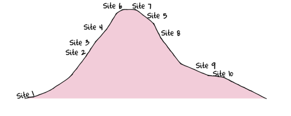
To assist with demonstrating Multidimensional Scaling (MDS), we will return to the fabricated species abundance data introduced in Tutorial 13.2. This data set comprises the abundances of 10 species within 10 sites located along a transect that extends in a northerly direction over a mountain range.
> set.seed(1)
> x <- seq(0,50,l=10)
> n <- 10
> sp1<-coenocline(x=x,A0=5,m=0,r=2,a=1,g=1,int=T, noise=T)
> sp2<-coenocline(x=x,A0=70,m=7,r=30,a=1,g=1,int=T, noise=T)
> sp3<-coenocline(x=x,A0=50,m=15,r=30,a=1,g=1,int=T, noise=T)
> sp4<-coenocline(x=x,A0=7,m=25,r=20,a=0.4,g=0.1,int=T, noise=T)
> sp5<-coenocline(x=x,A0=40,m=30,r=30,a=0.6,g=0.5,int=T, noise=T)
> sp6<-coenocline(x=x,A0=15,m=35,r=15,a=0.2,g=0.3,int=T, noise=T)
> sp7<-coenocline(x=x,A0=20,m=45,r=25,a=0.5,g=0.9,int=T, noise=T)
> sp8<-coenocline(x=x,A0=5,m=45,r=5,a=1,g=1,int=T, noise=T)
> sp9<-coenocline(x=x,A0=20,m=45,r=15,a=1,g=1,int=T, noise=T)
> sp10<-coenocline(x=x,A0=30,m=50,r=5,a=1,g=1,int=T, noise=T)
> X <- cbind(sp1, sp10,sp9,sp2,sp3,sp8,sp4,sp5,sp7,sp6)
> #X<-X[c(1,10,9,2,3,8,4,5,7,6),]
> colnames(X) <- paste("Sp",1:10,sep="")
> rownames(X) <- paste("Site", c(1,10,9,2,3,8,4,5,7,6), sep="")
> X <- X[c(1,4,5,7,8,10,9,6,3,2),]
> data <- data.frame(Sites=factor(rownames(X),levels=rownames(X)), X)
| Sites | Sp1 | Sp2 | Sp3 | Sp4 | Sp5 | Sp6 | Sp7 | Sp8 | Sp9 | Sp10 |
|---|---|---|---|---|---|---|---|---|---|---|
| Site1 | 5 | 0 | 0 | 65 | 5 | 0 | 0 | 0 | 0 | 0 |
| Site2 | 0 | 0 | 0 | 25 | 39 | 0 | 6 | 23 | 0 | 0 |
| Site3 | 0 | 0 | 0 | 6 | 42 | 0 | 6 | 31 | 0 | 0 |
| Site4 | 0 | 0 | 0 | 0 | 0 | 0 | 0 | 40 | 0 | 14 |
| Site5 | 0 | 0 | 6 | 0 | 0 | 0 | 0 | 34 | 18 | 12 |
| Site6 | 0 | 29 | 12 | 0 | 0 | 0 | 0 | 0 | 22 | 0 |
| Site7 | 0 | 0 | 21 | 0 | 0 | 5 | 0 | 0 | 20 | 0 |
| Site8 | 0 | 0 | 0 | 0 | 13 | 0 | 6 | 37 | 0 | 0 |
| Site9 | 0 | 0 | 0 | 60 | 47 | 0 | 4 | 0 | 0 | 0 |
| Site10 | 0 | 0 | 0 | 72 | 34 | 0 | 0 | 0 | 0 | 0 |
> set.seed(1)
> Site <- gl(10,1,10,lab=paste('Site',1:10, sep=""))
> Y <- matrix(c(
+ 6.1,4.2,101325,2,
+ 6.7,9.2,101352,510,
+ 6.8,8.6,101356,546,
+ 7.0,7.4,101372,758,
+ 7.2,5.8,101384,813,
+ 7.5,8.4,101395,856,
+ 7.5,0.5,101396,854,
+ 7.0,11.8,101370,734,
+ 8.4,8.2,101347,360,
+ 6.2,1.5,101345,356
+   ),10,4, byrow=TRUE)
> colnames(Y) <- c('pH','Slope', 'Pressure', 'Altitude')
> Substrate <- factor(c('Quartz','Shale','Shale','Shale','Shale','Quartz','Quartz','Shale','Quartz','Quartz'))
> enviro <- data.frame(Site,Y,Substrate)
| Site | pH | Slope | Pressure | Altitude | Substrate |
|---|---|---|---|---|---|
| Site1 | 6 | 4 | 101325 | 2 | Quartz |
| Site2 | 7 | 9 | 101352 | 510 | Shale |
| Site3 | 7 | 9 | 101356 | 546 | Shale |
| Site4 | 7 | 7 | 101372 | 758 | Shale |
| Site5 | 7 | 6 | 101384 | 813 | Shale |
| Site6 | 8 | 8 | 101395 | 856 | Quartz |
| Site7 | 8 | 0 | 101396 | 854 | Quartz |
| Site8 | 7 | 12 | 101370 | 734 | Shale |
| Site9 | 8 | 8 | 101347 | 360 | Quartz |
| Site10 | 6 | 2 | 101345 | 356 | Quartz |
At the end of the previous tutorial, we started to explore the relationships between community patterns and concurrently measured environmental data. To that end, we also regressed the first few principle components against environmental variables in Tutorial 14.2 and Tutorial 14.3. Tutorial 14.4 took the process of incorporating environmental predictors one step further by constraining the axis rotation process by the environmental variables. Nevertheless, in each case we are essentially exploring the (associations) effects of the environmental in reduced ordinal space. That is, we are investigating how the environmental variables relate to SOME of the patterns in the community data.
There are a number of techniques available for relating community data to environmental data without having to go via ordination. Each of these techniques explores relationships between the environmental data and the community distance matrix. Since the values in a distance (dissimilarity) matrix are not independent of one another (nor the same size as a regular predictor variable), regular modelling techniques cannot be employed. Instead, all of the techniques employ permutation tests. This tutorial will illustrate a couple of the most useful techniques.
Permutation (randomization) tests
Permutation (randomization) tests proceed by calculating a test statistic of some kind. This test statistic can be anything, but is usually a measure of effect, difference, association etc and is typically analogous to those used in regular statistical analyses. Where permutation tests diverge from regular hypothesis tests is that rather than base inferences on comparing the test statistic to a mathematical distribution representing the expected density of possible values when the null hypothesis is true, the test statistic is compared to a distribution created entirely and specifically for the observed data.
If the null hypothesis is really true (and there is no effect, association or pattern etc), then any arrangement (reshuffle) of the data should be just as likely to yield a test statistic as large as the actual one observed from the original data. Therefore, by repeatedly shuffling the data (or residuals) and each time generating the test statistic, we can build up a distribution of possible test statistic values for when the null hypothesis is true. This distribution of course includes the original test statistic value.
Null hypotheses can thus be tested by calculating the proportion of times the randomized/permuted test statistics (including the original test statistic value) are greater or equal to your original test statistic. This proportion is the equivalent of a p-value. Using the data to generate a custom reference distribution frees the analysis up from many of the assumptions that restrict parametric tests (such as normality and independence). However, the p-value is a proportion of the number of permutations, its resolution is dependent on the number of permutations and thus sample size. For example, there are only 5 rows in your data set, then there are a total of 120 ways to reorder the values in one of the columns. Consequently, the smallest p-value possible is $1/120=0.008$. More generally, permutation tests are less powerful (more conservative) than regular parametric tests. Moreover, the hypotheses they test do not strictly pertain to populations. Rather they are testing how likely an outcome could occur by chance.
Permutation test are so called because they generate a test statistic for each permutation (unique combination of values) of the data. Obviously, the original data is just one possible permulation. When the number of unique combinations in which the data can be rearranged gets very large (i.e. from large data sets) it is often not necessary to survey them all. Instead, it is often sufficient to sample a random selection (hence the alternative name - randomization test).
Mantel test
The Mantel test explores the correlation between two distance matrices. The two matrices are first flattered out into vectors and the Pearson product-moment correlation coefficient ($R$) is calculated. To assess the 'significance' (probability that population $R=0$) of this correlation coefficient is tested via a permutation procedure in which one of the vectors is repeatedly shuffled (random permutations) and the correlation coefficient recalculated after each permutation. The p-value is then calculated as the proportion of permuted $R$ values that are higher than (or equal to) the observed $R$ value.
In R, the Mantel test is supported by the mantel() function in the vegan package. As input, the mantel() function takes two distance matrices.
For this exercise we will prepare the community and environmental data according to:
- community data - square root transform followed by a Wisconsin double standardization and then a Bray-Curtis dissimilarity matrix
> data.dist <- vegdist(wisconsin(sqrt(data[,-1])),"bray")
> data.dist
Site1 Site2 Site3 Site4 Site2 0.67588 Site3 0.76402 0.08815 Site4 1.00000 0.76729 0.71733 Site5 1.00000 0.76729 0.71950 0.43782 Site6 1.00000 1.00000 1.00000 1.00000 Site7 1.00000 1.00000 1.00000 1.00000 Site8 0.85671 0.24898 0.18482 0.61339 Site9 0.52225 0.24045 0.30462 1.00000 Site10 0.43931 0.53961 0.60377 1.00000 Site5 Site6 Site7 Site8 Site2 Site3 Site4 Site5 Site6 0.56218 Site7 0.56218 0.40288 Site8 0.71950 1.00000 1.00000 Site9 1.00000 1.00000 1.00000 0.48944 Site10 1.00000 1.00000 1.00000 0.78859 Site9 Site2 Site3 Site4 Site5 Site6 Site7 Site8 Site9 Site10 0.29915 - environmental data - standardize each of the variables to a mean of 0 and a standard deviation of 1 and then a Euclidean distance matrix
> #since Substrate is a categorical variable, it first needs to be converted to a numeric
> # this could be done by first converting it into dummy variables or when there are only
> # two levels, a simple conversion to numeric will suffice.
> enviro1 <- within(enviro, Substrate <- as.numeric(Substrate))
> env.dist <- vegdist(decostand(enviro1[,-1],"standardize"),"euclid")
> env.dist
        1      2      3      4      5
2  3.3230
3  3.4352 0.3113
4  4.2004 1.4095 1.1200
5  4.6243 2.1315 1.8281 0.7722
6  4.9177 3.1669 2.9562 2.3098 2.1404
7  4.9080 4.0132 3.7487 3.0169 2.5116
8  4.5387 1.4067 1.3098 1.2431 1.8378
9  3.9401 3.2272 3.1427 3.3445 3.5238
10 1.7178 3.0392 3.0118 3.3462 3.5746
        6      7      8      9
2
3
4
5
6
7  2.2217
8  2.5329 3.9604
9  3.0373 3.7501 3.4269
10 3.9177 3.4388 4.0496 3.7782
Whilst the permutation aspect does free up some of the usual modelling assumptions (such as independence and normality), correlations are still inherently linear and therefore the relationships between the two matrices must also be linear. So our first step must be to explore the relationship between the two distance matrices using a scatterplot.
> plot(data.dist, env.dist)

So lets now perform the Mantel test with Pearson's product-moment correlation coefficient and a total of 1000 permutations.
> data.mantel <- mantel(data.dist, env.dist, perm=1000)
> data.mantel
Mantel statistic based on Pearson's product-moment correlation

Call:
mantel(xdis = data.dist, ydis = env.dist, permutations = 1000)

Mantel statistic r: 0.559
      Significance: 0.007

Upper quantiles of permutations (null model):
  90%   95% 97.5%   99%
0.225 0.305 0.358 0.465

Based on 1000 permutations
- The correlation between community distances and environmental distances is
0.56. - Of the 1000 random permutations only
7were equal to or greater than0.56(including the original $R$ value. We would therefore conclude that there is a relationship between community structure and the environmental variables. - For those who are not fixated on p-values, a range of upper confidence limits are also provided.
These limits represent the upper limits of various confidence ranges of the $R$ values. Hence the original $R$ value
is outside the upper 99% limit of
0.465
We can even examine a histogram of the permutational $R$ values and visualize how the original $R$ compares.
> hist(data.mantel$perm)
> abline(v=data.mantel$statistic)

- The probability distribution of $R$ is slightly skewed to the right rather than being a normal distribution. Nevertheless the observed $R$ value (indicated by the vertical line) is far to the right of this distribution and would therefore be considered a highly unusual outcome if the null hypothesis really was true.
Best subsets of environmental variables
The Mantel test investigates whether there is any evidence of a relationship between the patterns of community structure and and the patterns of environemntal variables. It does not single out the contributions of each of the environmental variables. In order to do so, we would need to iteratively go through all possible subsets (combinations) of the environmental variables and determine which subset correlates strongest with the community data.
The bioenv() function provides this very functionality by comparing the Spearman rank-based $R$ values from each combination of environmental predictors and selecting the combination with the highest $R$ value. This procedure is analogous to model selection in multiple regression.
Note, as input the bioenv() function expectes the community data to be a regular data matrix (not a distance matrix as it calls vegdist to create the distance matrix). Note also that the predictor variables must all be numeric (no factors). Factors should be first converted to a number (if there are only two levels) or to dummy codes.
> # convert the Substrate factor to a numeric via dummy coding
> # function definition at the start of this Tutorial
> enviro1 <- dummy(enviro[,-1])
Importantly, as the bioenv procedure fits models with multiple predictors (analogous to multiple regression), issues analogous to (multi)collinearity also apply. Specifically, when two or more predictors are correlated to one another, terms estimated later in a model tend to be underestimated as their trends have already been accounted for in earlier terms. Consequently, we need to ensure that the predictors are not correlated to one another. This can be assessed via scatterplot matricies, correlation matrices or more definitively, via variance inflation.
> library(car)
> vif(lm(1:nrow(enviro1) ~ pH+Slope+Pressure+Altitude+SubstrateShale, data=data.frame(enviro1)))
            pH          Slope
         1.976          2.188
      Pressure       Altitude
        45.805         52.754
SubstrateShale
         5.118
> vif(lm(1:nrow(enviro1) ~ pH+Slope+Altitude+SubstrateShale, data=data.frame(enviro1)))
            pH          Slope
         1.968          2.117
      Altitude SubstrateShale
         1.830          2.636
- Clearly there is an issue with the inclusion of both Pressure and Altitude. It is perhaps not surprising that Pressure and Altitude are related.
- Whilst neither Pressure nor Altitude are likely to be directly responsible for changes in community structure, Altitude is likely to be a closer conceptual proxy to a genuine ecological gradient - so Altitude will be retained at the expense of Pressure.
> # convert the Substrate factor to a numeric via dummy coding
> # function definition at the start of this Tutorial
> enviro1 <- dummy(enviro[,-1])
> #Pressure is now in column 3
> data.bioenv <- bioenv(wisconsin(sqrt(data[,-1])), decostand(enviro1[,-3],"standardize"))
> data.bioenv
Call:
bioenv(comm = wisconsin(sqrt(data[, -1])), env = decostand(enviro1[,      -3], "standardize"))

Subset of environmental variables with best correlation to community data.

Correlations:      spearman
Dissimilarities:   bray

Best model has 1 parameters (max. 4 allowed):
Altitude
with correlation  0.5515
- In this case, the best model contained just a single predictor (Altitude) which had a very strong association
(
0.5515) with the community data.
Note, this technique is best viewed as an exploratory variable selection tool. It does not perform inference testing, it just provides an empirical basis on which to justify exploring trends with subsets of environmental variables.
Permutational Multivariate Analaysis of Variance - adonis
Permutational Multivariate Analysis of Variance (adonis - or sometimes referred to as permutational MANOVA or nonparameteric MANOVA), partitions the total sums of squares of the multivariate data set (distance matrix) into the sequential contributions of each of the terms of a linear predictor (set of predictor variables perhaps with interactions).
Inference testing is conducted via permuted sequential sums of squares F-statistics generated from a large number of permutations of the raw data. When the distance matrix is Euclidean, the analysis is analogous to Redundancy Analysis (RDA). However, adonis is more flexible in that it can accommodate any distance matrix.
In R, adonis is supported via the adonis() function in the vegan package. The model is expressed as a formula of which the right hand side is a linear combination of predictors and the left hand side is either a distance matrix or a raw data frame. In the latter case, the data frame will be converted into a distance matrix via the vegdist() function
For reasons given above, we must avoid building models with predictors that are correlated to one another. In this case, we will exclude Pressure from the model.
> data.adonis <- adonis(data.dist ~ pH + Slope + Altitude + Substrate, data=enviro)
> data.adonis
Call:
adonis(formula = data.dist ~ pH + Slope + Altitude + Substrate,      data = enviro)

Terms added sequentially (first to last)

          Df SumsOfSqs MeanSqs F.Model
pH         1     0.219   0.219    1.63
Slope      1     0.560   0.560    4.16
Altitude   1     0.984   0.984    7.32
Substrate  1     0.384   0.384    2.86
Residuals  5     0.672   0.134
Total      9     2.819
             R2 Pr(>F)
pH        0.078  0.221
Slope     0.199  0.013 *
Altitude  0.349  0.001 ***
Substrate 0.136  0.045 *
Residuals 0.238
Total     1.000
---
Signif. codes:
  0 '***' 0.001 '**' 0.01 '*' 0.05
  '.' 0.1 ' ' 1
- Community patterns are associated with changes in slope, altitude and also substrate type.
There are numerous other techniques for testing hypotheses about the effects of individual factors on multivariate community data (notably, Analysis of Similarities or ANOSIM), yet these are less flexible (only handle single predictors) and tend to be more susceptible to heterogeneity and sample sizes.
Worked Examples
Basic statistics references
- Legendre and Legendre
- Quinn & Keough (2002) - Chpt 17
Mantel tests
Vare et al. (1995) measured the cover abundance of 44 plants from 24 sites so as to explore patterns in vegetation communities between these sites. They also measured a number of environmental variables (mainly concentration or various soil chemicals) from each site so as to also be able to characterise sites according to soil characteristics. Their primary interest was to investigate whether there was a correlation between the plant communities and the soil characteristics.
Download vareveg data set Download vareenv data set| Format of vareveg and vareenv data files | |||||||||||||||||||||||||||||||||||||||||||||||||||||||||
|---|---|---|---|---|---|---|---|---|---|---|---|---|---|---|---|---|---|---|---|---|---|---|---|---|---|---|---|---|---|---|---|---|---|---|---|---|---|---|---|---|---|---|---|---|---|---|---|---|---|---|---|---|---|---|---|---|---|
vareveg
| vareenv
|
> vareveg <- read.csv('../downloads/data/vareveg.csv')
> vareenv <- read.csv('../downloads/data/vareenv.csv')
- Briefly explore the two data sets and determine the appropriate sorts of standardizations and distance matrices
- Vegetation data
Show codeWhat combination of standardization and distance matrix would you recommend?
> #species means
> apply(vareveg[,-1],2, mean, na.rm=TRUE)
    C.vul   Emp.nig   Led.pal   Vac.myr
 1.877917  6.332917  0.349583  2.112917
  Vac.vit   Pin.syl   Des.fle   Bet.pub
11.459583  0.171250  0.233333  0.012083
  Vac.uli   Dip.mon    Dic.sp   Dic.fus
 0.634167  0.135000  1.687500  4.730000
  Dic.pol   Hyl.spl   Ple.sch   Pol.pil
 0.252500  0.751667 15.748750  0.025417
  Pol.jun   Pol.com   Poh.nut   Pti.cil
 0.577083  0.029583  0.109167  0.583750
  Bar.lyc   Cla.arb   Cla.ran   Cla.ste
 0.132917 10.627083 16.196250 20.279583
  Cla.unc   Cla.coc   Cla.cor   Cla.gra
 2.345000  0.116250  0.259167  0.214167
  Cla.fim   Cla.cri   Cla.chl   Cla.bot
 0.165000  0.311250  0.048333  0.019583
  Cla.ama    Cla.sp   Cet.eri   Cet.isl
 0.005833  0.021667  0.150000  0.084583
  Cet.niv   Nep.arc    Ste.sp   Pel.aph
 0.493750  0.219167  0.730000  0.031667
  Ich.eri   Cla.cer   Cla.def   Cla.phy
 0.009167  0.004167  0.426250  0.033333
> #species maximums
> apply(vareveg[,-1],2, max)
  C.vul Emp.nig Led.pal Vac.myr Vac.vit
  24.13   16.00    4.00   18.27   25.00
Pin.syl Des.fle Bet.pub Vac.uli Dip.mon
   1.20    3.70    0.25    8.10    2.07
 Dic.sp Dic.fus Dic.pol Hyl.spl Ple.sch
  23.43   37.07    3.00    9.97   70.03
Pol.pil Pol.jun Pol.com Poh.nut Pti.cil
   0.25    6.98    0.25    0.32   10.00
Bar.lyc Cla.arb Cla.ran Cla.ste Cla.unc
   3.00   39.00   59.00   84.30   23.68
Cla.coc Cla.cor Cla.gra Cla.fim Cla.cri
   0.25    1.42    0.50    0.25    1.78
Cla.chl Cla.bot Cla.ama  Cla.sp Cet.eri
   0.25    0.25    0.08    0.25    0.78
Cet.isl Cet.niv Nep.arc  Ste.sp Pel.aph
   0.67   10.03    4.87   10.28    0.33
Ich.eri Cla.cer Cla.def Cla.phy
   0.10    0.05    1.97    0.25
> #species sums
> apply(vareveg[,-1],2, sum, na.rm=TRUE)
  C.vul Emp.nig Led.pal Vac.myr Vac.vit
  45.07  151.99    8.39   50.71  275.03
Pin.syl Des.fle Bet.pub Vac.uli Dip.mon
   4.11    5.60    0.29   15.22    3.24
 Dic.sp Dic.fus Dic.pol Hyl.spl Ple.sch
  40.50  113.52    6.06   18.04  377.97
Pol.pil Pol.jun Pol.com Poh.nut Pti.cil
   0.61   13.85    0.71    2.62   14.01
Bar.lyc Cla.arb Cla.ran Cla.ste Cla.unc
   3.19  255.05  388.71  486.71   56.28
Cla.coc Cla.cor Cla.gra Cla.fim Cla.cri
   2.79    6.22    5.14    3.96    7.47
Cla.chl Cla.bot Cla.ama  Cla.sp Cet.eri
   1.16    0.47    0.14    0.52    3.60
Cet.isl Cet.niv Nep.arc  Ste.sp Pel.aph
   2.03   11.85    5.26   17.52    0.76
Ich.eri Cla.cer Cla.def Cla.phy
   0.22    0.10   10.23    0.80
> #species variance
> apply(vareveg[,-1],2, var, na.rm=TRUE)
    C.vul   Emp.nig   Led.pal   Vac.myr
2.488e+01 2.278e+01 9.328e-01 2.322e+01
  Vac.vit   Pin.syl   Des.fle   Bet.pub
3.882e+01 7.510e-02 5.834e-01 2.600e-03
  Vac.uli   Dip.mon    Dic.sp   Dic.fus
2.903e+00 1.847e-01 2.953e+01 8.290e+01
  Dic.pol   Hyl.spl   Ple.sch   Pol.pil
4.601e-01 5.763e+00 3.570e+02 3.774e-03
  Pol.jun   Pol.com   Poh.nut   Pti.cil
2.117e+00 4.700e-03 1.031e-02 4.165e+00
  Bar.lyc   Cla.arb   Cla.ran   Cla.ste
3.734e-01 1.124e+02 2.223e+02 8.595e+02
  Cla.unc   Cla.coc   Cla.cor   Cla.gra
2.468e+01 7.885e-03 7.913e-02 1.254e-02
  Cla.fim   Cla.cri   Cla.chl   Cla.bot
6.478e-03 1.823e-01 6.797e-03 2.726e-03
  Cla.ama    Cla.sp   Cet.eri   Cet.isl
3.210e-04 2.693e-03 4.372e-02 2.404e-02
  Cet.niv   Nep.arc    Ste.sp   Pel.aph
4.149e+00 9.838e-01 4.325e+00 6.867e-03
  Ich.eri   Cla.cer   Cla.def   Cla.phy
6.167e-04 1.471e-04 2.595e-01 7.101e-03
- Vegetation data
Show codeWhat combination of standardization and distance matrix would you recommend?
> #environmental variables means
> apply(vareenv[,-1],2, mean, variables.rm=TRUE)
       N        P        K       Ca
 22.3833  45.0792 162.9292 569.6625
      Mg        S       Al       Fe
 87.4583  37.1917 142.4750  49.6125
      Mn       Zn       Mo Baresoil
 49.3292   7.5958   0.3958  22.9492
Humdepth       pH
  2.2000   2.9333
> #environmental variables maximums > apply(vareenv[,-1],2, max)
       N        P        K       Ca
    33.1     73.5    313.8   1169.7
      Mg        S       Al       Fe
   209.1     60.2    435.1    204.4
      Mn       Zn       Mo Baresoil
   132.0     16.8      1.1     56.9
Humdepth       pH
     3.8      3.6
> #variable sums > apply(vareenv[,-1],2, sum, na.rm=TRUE)
       N        P        K       Ca
   537.2   1081.9   3910.3  13671.9
      Mg        S       Al       Fe
  2099.0    892.6   3419.4   1190.7
      Mn       Zn       Mo Baresoil
  1183.9    182.3      9.5    550.8
Humdepth       pH
    52.8     70.4
> #environmental variables variance > apply(vareenv[,-1],2, var, na.rm=TRUE)
        N         P         K        Ca
3.056e+01 2.234e+02 4.205e+03 5.933e+04
       Mg         S        Al        Fe
1.682e+03 1.361e+02 1.496e+04 3.654e+03
       Mn        Zn        Mo  Baresoil
1.150e+03 8.904e+00 5.759e-02 2.703e+02
 Humdepth        pH
4.417e-01 4.580e-02
- Vegetation data
- Actually there are not incorrect answers to the above questions. Each combination of standardizations and distance matrices will emphasize
a different aspect of the multivariate data sets. Indeed one of the attractions of Q-mode analyses is this very flexibility.
Perform the standardizations/distance matrices as indicated above.
Show code
> library(vegan)
> #species
> vareveg.std <- wisconsin(vareveg[,-1])
> vareveg.dist <- vegdist(vareveg.std, "bray")
> #environmental variables
> vareenv.std <- decostand(vareenv[,-1], "standardize")
> vareenv.dist <- vegdist(vareenv.std, "euc")
- Perform a Mantel test to calculate the correlation between the two matricies (vegetation and soil).
Show code
> library(vegan)
> mantel(vareveg.dist,vareenv.dist)
Mantel statistic based on Pearson's product-moment correlation Call: mantel(xdis = vareveg.dist, ydis = vareenv.dist) Mantel statistic r: 0.427 Significance: 0.001 Upper quantiles of permutations (null model): 90% 95% 97.5% 99% 0.160 0.202 0.230 0.276 Based on 999 permutations- What was the R value? Show code
> library(vegan)
> mantel(vareveg.dist,vareenv.dist)$statistic
[1] 0.4268
- Was this significant?
- What was the R value?
- Generate a correlogram (mutivariate correlation plot)
Show code
> par(mar=c(4,4,0,0))
> plot(vareenv.dist,vareveg.dist, ann=F, axes=F, type="n")
> points(vareenv.dist,vareveg.dist, pch=16)
> axis(1)
> axis(2, las=1)
> mtext("Vegetation distances",2,line=3)
> mtext("Soil chemistry distances",1,line=3)
> box(bty="l")

Adonis - Permutational Multivariate analysis of variance
In the previous question we established that there was an association between the vegetation community and the soil chemistry. In this question we are going to delve a little deeper into that association. Now there are numerous ways that we could do this, so we are going to just focus on two of those.
- perform a permutational multivariate analysis of variance (adonis) of the vegetation community against concentrations of certain soil chemicals
- perform a permutational multivariate analysis of variance (adonis) of the vegetation community against the PCA axes scores from the soil chemistry data
- Since the permulational multivariate analysis of variance partitions variance sequentially, it is important that all predictors are uncorrelated to one another (
or the effects of those later in the model will be under-estimated) - the (multi)collinearity issue.
Lets start by exploring the relationships amongst the soil chemistry variables
Show codeClearly Phosphorus, Potassium, Calcium, Magnessium, Sulfure and Zinc are correlated to one another and thus cannot all be in the model. Similarly, Iron, Aluminium, percent of baresoil, pH and humus depth are correlated to each other.> pairs(vareenv[,-1])

- We might
elect to include one as a representative from each of these groups along with Nitrogen in a model. Ideally we would base our selection on some sort of
meaningful criteria. In the absence of anything even vaguely sensible around here, we will try the combination of Nitrogen, Calcium and Iron. Lets try it.
Show code
> adonis(vareveg.dist~N+Ca+Fe, data=vareenv)
Call: adonis(formula = vareveg.dist ~ N + Ca + Fe, data = vareenv) Terms added sequentially (first to last) Df SumsOfSqs MeanSqs F.Model N 1 0.27 0.267 1.70 Ca 1 0.38 0.381 2.42 Fe 1 0.30 0.303 1.93 Residuals 20 3.14 0.157 Total 23 4.09 R2 Pr(>F) N 0.065 0.060 . Ca 0.093 0.005 ** Fe 0.074 0.034 * Residuals 0.768 Total 1.000 --- Signif. codes: 0 '***' 0.001 '**' 0.01 '*' 0.05 '.' 0.1 ' ' 1 - The alternative approach introduced earlier is to create a triplet of soil chemistry predictors from PCA. Lets have a try
Show codeNote this has not necessarily told us a great deal more. All we have established is that there may well be three important gradients underlying the chemical ecosystem and that these many influence the vegetation communities.
> vareenv.pca <- rda(vareenv[,-1], scale=TRUE)
> adonis(vareveg.dist~scores(vareenv.pca,1)$sites+scores(vareenv.pca,2)$sites+scores(vareenv.pca,3)$sites)
Call:
adonis(formula = vareveg.dist ~ scores(vareenv.pca, 1)$sites +      scores(vareenv.pca, 2)$sites + scores(vareenv.pca, 3)$sites)

Terms added sequentially (first to last)

                             Df
scores(vareenv.pca, 1)$sites  1
scores(vareenv.pca, 2)$sites  1
scores(vareenv.pca, 3)$sites  1
Residuals                    20
Total                        23
                             SumsOfSqs
scores(vareenv.pca, 1)$sites      0.46
scores(vareenv.pca, 2)$sites      0.41
scores(vareenv.pca, 3)$sites      0.25
Residuals                         2.98
Total                             4.09
                             MeanSqs
scores(vareenv.pca, 1)$sites   0.461
scores(vareenv.pca, 2)$sites   0.406
scores(vareenv.pca, 3)$sites   0.249
Residuals                      0.149
Total
                             F.Model
scores(vareenv.pca, 1)$sites    3.09
scores(vareenv.pca, 2)$sites    2.72
scores(vareenv.pca, 3)$sites    1.67
Residuals
Total
                                R2
scores(vareenv.pca, 1)$sites 0.113
scores(vareenv.pca, 2)$sites 0.099
scores(vareenv.pca, 3)$sites 0.061
Residuals                    0.728
Total                        1.000
                             Pr(>F)
scores(vareenv.pca, 1)$sites  0.001 ***
scores(vareenv.pca, 2)$sites  0.002 **
scores(vareenv.pca, 3)$sites  0.050 *
Residuals
Total
---
Signif. codes:
  0 '***' 0.001 '**' 0.01 '*' 0.05
  '.' 0.1 ' ' 1
Permutational Multivariate analysis of variance
Jongman et al. (1987) presented a data set from a study in which the cover abundance of 30 plant species were measured on 20 rangeland dune sites. They also indicated what the form of management each site experienced (either biological farming, hobby farming, nature conservation management or standard farming. The major intension of the study was to determine whether the vegetation communities differed between the alternative management practices.
Download dune data set| Format of dune.csv data file | |||||||||||||||||||||||||||||
|---|---|---|---|---|---|---|---|---|---|---|---|---|---|---|---|---|---|---|---|---|---|---|---|---|---|---|---|---|---|
|
 |
> dune <- read.csv('../downloads/data/dune.csv')
> dune
   MANAGEMENT Belper Empnig Junbuf
1          BF      3      0      0
2          SF      0      0      3
3          SF      2      0      0
4          SF      0      0      0
5          HF      0      0      0
6          SF      0      0      0
7          HF      0      0      0
8          HF      2      0      0
9          NM      0      0      0
10         NM      0      0      0
11         BF      2      0      0
12         BF      0      0      0
13         HF      0      0      4
14         NM      2      0      0
15         SF      2      0      0
16         NM      0      0      0
17         NM      0      0      0
18         NM      0      2      0
19         SF      0      0      4
20         HF      0      0      2
   Junart Airpra Elepal Rumace Viclat
1       0      0      0      0      0
2       0      0      0      0      0
3       0      0      0      0      0
4       3      0      8      0      0
5       0      0      0      6      0
6       0      0      0      0      0
7       4      0      4      0      0
8       0      0      0      5      0
9       0      2      0      0      0
10      3      0      5      0      0
11      0      0      0      0      1
12      0      0      0      0      2
13      4      0      0      2      0
14      0      0      0      0      1
15      0      0      0      0      0
16      4      0      4      0      0
17      0      0      4      0      0
18      0      3      0      0      0
19      0      0      0      2      0
20      0      0      0      3      0
   Brarut Ranfla Cirarv Hyprad Leoaut
1       0      0      0      0      5
2       0      2      0      0      2
3       2      0      2      0      2
4       4      2      0      0      0
5       6      0      0      0      3
6       0      0      0      0      0
7       2      2      0      0      3
8       2      0      0      0      3
9       0      0      0      2      2
10      4      2      0      0      2
11      2      0      0      0      3
12      4      0      0      2      5
13      2      0      0      0      2
14      6      0      0      0      5
15      2      0      0      0      2
16      4      4      0      0      2
17      0      2      0      0      2
18      3      0      0      5      6
19      4      0      0      0      2
20      2      0      0      0      3
   Potpal Poapra Calcus Tripra Trirep
1       0      4      0      0      5
2       0      2      0      0      2
3       0      4      0      0      1
4       0      0      3      0      0
5       0      3      0      5      5
6       0      4      0      0      0
7       0      4      0      0      2
8       0      2      0      2      2
9       0      1      0      0      0
10      2      0      0      0      1
11      0      4      0      0      6
12      0      4      0      0      3
13      0      4      0      0      3
14      0      3      0      0      2
15      0      5      0      0      2
16      0      0      3      0      0
17      2      0      4      0      6
18      0      0      0      0      2
19      0      0      0      0      3
20      0      4      0      2      2
   Antodo Salrep Achmil Poatri Chealb
1       0      0      3      7      0
2       0      0      0      9      1
3       0      0      0      5      0
4       0      0      0      2      0
5       3      0      2      4      0
6       0      0      1      2      0
7       0      0      0      4      0
8       4      0      2      6      0
9       4      0      2      0      0
10      0      0      0      0      0
11      4      0      4      4      0
12      0      0      0      0      0
13      0      0      0      5      0
14      0      3      0      0      0
15      0      0      0      6      0
16      0      5      0      0      0
17      0      0      0      0      0
18      4      3      0      0      0
19      0      0      0      4      0
20      2      0      2      5      0
   Elyrep Sagpro Plalan Agrsto Lolper
1       4      0      0      0      5
2       0      2      0      5      0
3       4      5      0      8      5
4       0      0      0      7      0
5       0      0      5      0      6
6       4      0      0      0      7
7       0      2      0      4      4
8       4      0      5      0      2
9       0      0      2      0      0
10      0      0      0      4      0
11      0      0      3      0      6
12      0      2      3      0      7
13      6      2      0      3      2
14      0      0      3      0      2
15      4      0      0      4      6
16      0      0      0      5      0
17      0      0      0      4      0
18      0      3      0      0      0
19      0      4      0      4      0
20      0      0      5      0      6
   Alogen Brohor
1       2      4
2       5      0
3       2      3
4       4      0
5       0      0
6       0      0
7       5      0
8       0      2
9       0      0
10      0      0
11      0      4
12      0      0
13      3      0
14      0      0
15      7      0
16      0      0
17      0      0
18      0      0
19      8      0
20      0      2
-
Briefly explore the dune data set and determine the appropriate sort of standardization and distance index
Show codeWhilst the means, maximums and variances are mostly fairly similar, there are some species such as Chealb and Empnig that are an order of magnitude less abundant and variable than the bulk of the species. Therefore a Wisconsin double standardization would still be appropriate. A Bray-Curtis dissimilarity would thence be a good choice.
> #species means
> apply(dune[,-1],2, mean, na.rm=TRUE)
Belper Empnig Junbuf Junart Airpra
  0.65   0.10   0.65   0.90   0.25
Elepal Rumace Viclat Brarut Ranfla
  1.25   0.90   0.20   2.45   0.70
Cirarv Hyprad Leoaut Potpal Poapra
  0.10   0.45   2.70   0.20   2.40
Calcus Tripra Trirep Antodo Salrep
  0.50   0.45   2.35   1.05   0.55
Achmil Poatri Chealb Elyrep Sagpro
  0.80   3.15   0.05   1.30   1.00
Plalan Agrsto Lolper Alogen Brohor
  1.30   2.40   2.90   1.80   0.75
> #species maximums
> apply(dune[,-1],2, max)
Belper Empnig Junbuf Junart Airpra
     3      2      4      4      3
Elepal Rumace Viclat Brarut Ranfla
     8      6      2      6      4
Cirarv Hyprad Leoaut Potpal Poapra
     2      5      6      2      5
Calcus Tripra Trirep Antodo Salrep
     4      5      6      4      5
Achmil Poatri Chealb Elyrep Sagpro
     4      9      1      6      5
Plalan Agrsto Lolper Alogen Brohor
     5      8      7      8      4
> #species sums > apply(dune[,-1],2, sum, na.rm=TRUE)
Belper Empnig Junbuf Junart Airpra
    13      2     13     18      5
Elepal Rumace Viclat Brarut Ranfla
    25     18      4     49     14
Cirarv Hyprad Leoaut Potpal Poapra
     2      9     54      4     48
Calcus Tripra Trirep Antodo Salrep
    10      9     47     21     11
Achmil Poatri Chealb Elyrep Sagpro
    16     63      1     26     20
Plalan Agrsto Lolper Alogen Brohor
    26     48     58     36     15
> #species variance > apply(dune[,-1],2, var, na.rm=TRUE)
Belper Empnig Junbuf Junart Airpra
1.0816 0.2000 1.9237 2.6211 0.6184
Elepal Rumace Viclat Brarut Ranfla
5.5658 3.2526 0.2737 3.6289 1.3789
Cirarv Hyprad Leoaut Potpal Poapra
0.2000 1.5237 2.4316 0.3789 3.4105
Calcus Tripra Trirep Antodo Salrep
1.5263 1.5237 3.6079 2.8921 1.9447
Achmil Poatri Chealb Elyrep Sagpro
1.5368 7.9237 0.0500 4.3263 2.4211
Plalan Agrsto Lolper Alogen Brohor
3.8000 7.2000 7.9895 6.9053 1.9868
- Perform the aforementioned standardization and distance measure procedures.
Show code
> library(vegan)
> dune.dist <- vegdist(wisconsin(dune[,-1]), "bray")
- Now perform the permutational multivariate analysis of variance relating the dune vegetation communities to the management practices.
Show code
> dune.adonis<-adonis(dune.dist~dune[,1])
> dune.adonis
Call: adonis(formula = dune.dist ~ dune[, 1]) Terms added sequentially (first to last) Df SumsOfSqs MeanSqs F.Model dune[, 1] 3 1.42 0.473 2.31 Residuals 16 3.28 0.205 Total 19 4.70 R2 Pr(>F) dune[, 1] 0.302 0.006 ** Residuals 0.698 Total 1.000 --- Signif. codes: 0 '***' 0.001 '**' 0.01 '*' 0.05 '.' 0.1 ' ' 1 -
The above analysis indicates that the dune vegetation communities do indeed differ between the different management practices. However, we may wish
to explore whether the alternative farming practices (BF: biological farming, HF: hobby farming, and NM: natural conservation management) each differ in communities
from the standard farming practices (SF).
We can do this by generating dummy codes for the managemnet variable and defining treatment contrasts relative to the SF level.
Show code> management <-factor(dune$MANAGEMENT, levels=c("SF","BF","HF","NM")) > mm <- model.matrix(~management) > colnames(mm) <-gsub("management","",colnames(mm)) > mm <- data.frame(mm) > dune.adonis<-adonis(dune.dist~BF+HF+NM, data=mm) > dune.adonis
Call:
adonis(formula = dune.dist ~ BF + HF + NM, data = mm)

Terms added sequentially (first to last)

          Df SumsOfSqs MeanSqs F.Model
BF         1      0.33   0.334    1.63
HF         1      0.38   0.376    1.84
NM         1      0.71   0.709    3.47
Residuals 16      3.28   0.205
Total     19      4.70
             R2 Pr(>F)
BF        0.071  0.116
HF        0.080  0.097 .
NM        0.151  0.010 **
Residuals 0.698
Total     1.000
---
Signif. codes:
  0 '***' 0.001 '**' 0.01 '*' 0.05
  '.' 0.1 ' ' 1
Permutational multivariate analysis of variance
Mac Nally (1989) studied geographic variation in forest bird communities. His data set consists of the maximum abundance for 102 bird species from 37 sites that where further classified into five different forest types (Gippsland manna gum, montane forest, woodland, box-ironbark and river redgum and mixed forest). He was primarily interested in determining whether the bird assemblages differed between forest types.
In Tutorial 15.1 we explored the bird communities using non-metric multidimensional scaling. We then overlay the environmental habitat variable with a permutation test that explored the association of the habitat levels with the ordination axes. That is, we investigate the degree to which a treatment (habitat level) aligns with the axes.
Alternatively, we could use a multivariate analysis of variance approach to investigate the effects of habitat on the bird community structure.
Download the macnally data set| Format of macnally_full.csv data file | |||||||||||||||||||||||||||||
|---|---|---|---|---|---|---|---|---|---|---|---|---|---|---|---|---|---|---|---|---|---|---|---|---|---|---|---|---|---|
|
 |
> macnally <- read.csv('../downloads/data/macnally_full.csv')
> macnally
HABITAT GST
Reedy Lake Mixed 3.4
Pearcedale Gipps.Manna 3.4
Warneet Gipps.Manna 8.4
Cranbourne Gipps.Manna 3.0
Lysterfield Mixed 5.6
Red Hill Mixed 8.1
Devilbend Mixed 8.3
Olinda Mixed 4.6
Fern Tree Gum Montane Forest 3.2
Sherwin Foothills Woodland 4.6
Heathcote Ju Montane Forest 3.7
Warburton Montane Forest 3.8
Millgrove Mixed 5.4
Ben Cairn Mixed 3.1
Panton Gap Montane Forest 3.8
OShannassy Mixed 9.6
Ghin Ghin Mixed 3.4
Minto Mixed 5.6
Hawke Mixed 1.7
St Andrews Foothills Woodland 4.7
Nepean Foothills Woodland 14.0
Cape Schanck Mixed 6.0
Balnarring Mixed 4.1
Bittern Gipps.Manna 6.5
Bailieston Box-Ironbark 6.5
Donna Buang Mixed 1.5
Upper Yarra Mixed 4.7
Gembrook Mixed 7.5
Arcadia River Red Gum 3.1
Undera River Red Gum 2.7
Coomboona River Red Gum 4.4
Toolamba River Red Gum 3.0
Rushworth Box-Ironbark 2.1
Sayers Box-Ironbark 2.6
Waranga Mixed 3.0
Costerfield Box-Ironbark 7.1
Tallarook Foothills Woodland 4.3
EYR GF BTH GWH WTTR
Reedy Lake 0.0 0.0 0.0 0.0 0.0
Pearcedale 9.2 0.0 0.0 0.0 0.0
Warneet 3.8 0.7 2.8 0.0 0.0
Cranbourne 5.0 0.0 5.0 2.0 0.0
Lysterfield 5.6 12.9 12.2 9.5 2.1
Red Hill 4.1 10.9 24.5 5.6 6.7
Devilbend 7.1 6.9 29.1 4.2 2.0
Olinda 5.3 11.1 28.2 3.9 6.5
Fern Tree Gum 5.2 8.3 18.2 3.8 4.2
Sherwin 1.2 4.6 6.5 2.3 5.2
Heathcote Ju 2.5 6.3 24.9 2.8 7.4
Warburton 6.5 11.1 36.1 6.2 8.5
Millgrove 6.5 11.9 19.6 3.3 8.6
Ben Cairn 9.3 11.1 25.9 9.3 8.3
Panton Gap 3.8 10.3 34.6 7.9 4.8
OShannassy 4.0 5.4 34.9 7.0 5.1
Ghin Ghin 2.7 9.1 16.1 1.3 3.2
Minto 3.3 13.3 28.0 7.0 8.3
Hawke 2.6 5.5 16.0 4.3 6.7
St Andrews 3.6 6.0 25.2 3.7 7.5
Nepean 5.6 5.5 20.0 3.0 6.6
Cape Schanck 4.9 4.9 16.2 3.4 2.6
Balnarring 4.9 10.7 21.2 3.9 0.0
Bittern 9.7 7.8 14.4 5.2 0.0
Bailieston 2.5 5.1 5.6 4.3 5.7
Donna Buang 0.0 2.2 9.6 6.7 3.0
Upper Yarra 3.1 7.0 17.1 8.3 12.8
Gembrook 7.5 12.7 16.4 4.7 6.4
Arcadia 0.0 1.2 0.0 1.2 0.0
Undera 0.0 2.2 0.0 1.3 6.5
Coomboona 0.0 2.1 0.0 0.0 3.3
Toolamba 0.0 0.5 0.0 0.8 0.0
Rushworth 1.1 3.2 1.8 0.5 4.8
Sayers 0.0 1.1 7.5 1.6 5.2
Waranga 1.6 1.5 3.0 0.0 3.0
Costerfield 2.2 4.5 9.0 2.7 6.0
Tallarook 2.9 8.7 14.4 2.9 5.8
WEHE WNHE SFW WBSW CR
Reedy Lake 0.0 11.9 0.4 0.0 1.1
Pearcedale 0.0 11.5 8.3 12.6 0.0
Warneet 10.7 12.3 4.9 10.7 0.0
Cranbourne 3.0 10.0 6.9 12.0 0.0
Lysterfield 7.9 28.6 9.2 5.0 19.1
Red Hill 9.4 6.7 0.0 8.9 12.1
Devilbend 7.1 27.4 13.1 2.8 0.0
Olinda 2.6 10.9 3.1 8.6 9.3
Fern Tree Gum 2.8 9.0 3.8 5.6 14.1
Sherwin 0.6 3.6 3.8 3.0 7.5
Heathcote Ju 1.3 4.7 5.5 9.5 5.7
Warburton 2.3 25.4 8.2 5.9 10.5
Millgrove 2.5 11.9 4.3 5.4 10.8
Ben Cairn 2.8 2.8 2.8 8.3 18.5
Panton Gap 2.9 3.7 4.8 7.2 5.9
OShannassy 2.6 6.4 3.9 11.3 11.6
Ghin Ghin 4.7 0.0 22.0 5.8 7.4
Minto 7.0 38.9 10.5 7.0 14.0
Hawke 3.5 5.9 6.7 10.0 3.7
St Andrews 4.7 10.0 0.0 0.0 4.0
Nepean 7.0 3.3 7.0 10.0 4.7
Cape Schanck 2.8 9.4 6.6 7.8 5.1
Balnarring 5.1 2.9 12.1 6.1 0.0
Bittern 11.5 12.5 20.7 4.9 0.0
Bailieston 6.2 6.2 1.2 0.0 0.0
Donna Buang 8.1 0.0 0.0 7.3 8.1
Upper Yarra 1.3 6.4 2.3 5.4 5.4
Gembrook 1.6 8.9 9.3 6.4 4.8
Arcadia 0.0 1.8 0.7 0.0 0.0
Undera 0.0 0.0 6.5 0.0 0.0
Coomboona 0.0 0.0 0.8 0.0 0.0
Toolamba 0.0 0.0 1.6 0.0 0.0
Rushworth 0.9 5.3 4.8 0.0 1.1
Sayers 3.6 6.9 6.7 0.0 2.7
Waranga 0.0 14.5 6.7 0.0 0.7
Costerfield 2.5 7.7 9.5 0.0 7.7
Tallarook 2.8 11.1 2.9 0.0 3.8
LK RWB AUR STTH LR
Reedy Lake 3.8 9.7 0.0 0.0 4.8
Pearcedale 0.5 11.6 0.0 0.0 3.7
Warneet 1.9 16.6 2.3 2.8 5.5
Cranbourne 2.0 11.0 1.5 0.0 11.0
Lysterfield 3.6 5.7 8.8 7.0 1.6
Red Hill 6.7 2.7 0.0 16.8 3.4
Devilbend 2.8 2.4 2.8 13.9 0.0
Olinda 3.8 0.6 1.3 10.2 0.0
Fern Tree Gum 3.2 0.0 0.0 12.2 0.6
Sherwin 2.4 0.6 0.0 11.3 5.8
Heathcote Ju 2.9 0.0 1.8 12.0 0.0
Warburton 3.1 9.8 1.6 7.6 15.0
Millgrove 6.5 2.7 2.0 8.6 0.0
Ben Cairn 3.1 0.0 3.1 12.0 3.3
Panton Gap 3.1 0.6 3.8 17.3 2.4
OShannassy 2.3 0.0 2.3 7.8 0.0
Ghin Ghin 4.5 0.0 0.0 8.1 2.7
Minto 5.2 1.7 5.2 25.2 0.0
Hawke 2.1 0.5 1.5 9.0 4.8
St Andrews 5.1 2.8 3.7 15.8 3.4
Nepean 3.3 2.1 3.7 12.0 2.2
Cape Schanck 5.2 21.3 0.0 0.0 4.3
Balnarring 2.7 0.0 0.0 4.9 16.5
Bittern 0.0 16.1 5.2 0.0 0.0
Bailieston 1.6 5.0 4.1 9.8 0.0
Donna Buang 1.5 2.2 0.7 5.2 0.0
Upper Yarra 2.4 0.6 2.3 6.4 0.0
Gembrook 3.6 14.5 4.7 24.3 2.4
Arcadia 1.8 0.0 2.5 0.0 2.7
Undera 0.0 0.0 2.2 7.5 3.1
Coomboona 2.8 0.0 2.2 3.1 1.7
Toolamba 2.0 0.0 2.5 0.0 2.5
Rushworth 1.1 26.3 1.6 3.2 0.0
Sayers 1.6 8.0 1.6 7.5 2.7
Waranga 4.0 23.0 1.6 0.0 8.9
Costerfield 2.2 8.9 1.9 9.3 1.1
Tallarook 2.9 2.9 1.9 4.6 10.3
WPHE YTH ER PCU ESP
Reedy Lake 27.3 0.0 5.1 0.0 0.0
Pearcedale 27.6 0.0 2.7 0.0 3.7
Warneet 27.5 0.0 5.3 0.0 0.0
Cranbourne 20.0 0.0 2.1 0.0 2.0
Lysterfield 0.0 0.0 1.4 0.0 3.5
Red Hill 0.0 0.0 2.2 0.0 3.4
Devilbend 16.7 0.0 0.0 0.0 5.5
Olinda 0.0 0.0 1.2 0.0 5.1
Fern Tree Gum 0.0 0.0 1.3 2.8 7.1
Sherwin 0.0 9.6 2.3 2.9 0.6
Heathcote Ju 0.0 0.0 0.0 2.8 0.9
Warburton 0.0 0.0 0.0 1.8 7.6
Millgrove 0.0 0.0 6.5 2.5 5.4
Ben Cairn 0.0 0.0 0.0 2.5 7.4
Panton Gap 0.0 0.0 0.0 3.1 9.2
OShannassy 0.0 0.0 0.0 1.5 3.1
Ghin Ghin 8.4 8.4 3.4 0.0 0.0
Minto 15.4 0.0 0.0 0.0 3.3
Hawke 0.0 0.0 0.0 2.1 3.7
St Andrews 0.0 9.0 0.0 3.7 5.6
Nepean 0.0 0.0 3.7 0.0 4.0
Cape Schanck 0.0 0.0 6.4 0.0 4.6
Balnarring 0.0 0.0 9.1 0.0 3.9
Bittern 27.7 0.0 2.3 0.0 0.0
Bailieston 0.0 8.7 0.0 0.0 0.0
Donna Buang 0.0 0.0 0.0 1.5 7.4
Upper Yarra 0.0 0.0 0.0 1.3 2.3
Gembrook 0.0 0.0 3.6 0.0 26.6
Arcadia 27.6 0.0 4.3 3.7 0.0
Undera 13.5 11.5 2.0 0.0 0.0
Coomboona 13.9 5.6 4.6 1.1 0.0
Toolamba 16.0 0.0 5.0 0.0 0.0
Rushworth 0.0 10.7 3.2 0.0 0.0
Sayers 0.0 20.2 1.1 0.0 0.0
Waranga 25.3 2.2 3.4 0.0 0.0
Costerfield 0.0 15.8 1.1 0.0 0.0
Tallarook 0.0 2.9 0.0 0.0 5.8
SCR RBFT BFCS WAG WWCH
Reedy Lake 0.0 0.0 0.6 1.9 0.0
Pearcedale 0.0 1.1 1.1 3.4 0.0
Warneet 0.0 0.0 1.5 2.1 0.0
Cranbourne 0.0 5.0 1.4 3.4 0.0
Lysterfield 0.7 0.0 2.7 0.0 0.0
Red Hill 0.0 0.7 2.0 0.0 0.0
Devilbend 0.0 0.0 3.6 0.0 0.0
Olinda 0.0 0.7 0.0 0.0 0.0
Fern Tree Gum 0.0 1.9 0.6 0.0 0.0
Sherwin 3.0 0.0 1.2 0.0 9.8
Heathcote Ju 2.6 0.0 0.0 0.0 11.7
Warburton 0.0 0.9 1.5 0.0 0.0
Millgrove 2.0 5.4 2.2 0.0 0.0
Ben Cairn 0.0 0.0 0.0 0.0 0.0
Panton Gap 0.0 3.7 0.0 0.0 0.0
OShannassy 0.0 9.6 0.7 0.0 0.0
Ghin Ghin 0.0 44.7 0.4 1.3 0.0
Minto 0.0 10.5 0.0 0.0 0.0
Hawke 0.0 0.0 0.7 0.0 3.2
St Andrews 4.0 0.9 0.0 0.0 10.0
Nepean 2.0 0.0 1.1 0.0 0.0
Cape Schanck 0.0 3.4 0.0 0.0 0.0
Balnarring 0.0 2.7 1.0 0.0 0.0
Bittern 0.0 2.3 2.3 6.3 0.0
Bailieston 6.2 0.0 1.6 0.0 10.0
Donna Buang 0.0 0.0 1.5 0.0 0.0
Upper Yarra 0.0 6.4 0.9 0.0 0.0
Gembrook 4.7 2.8 0.0 0.0 0.0
Arcadia 0.0 0.6 2.1 4.9 8.0
Undera 0.0 0.0 1.9 2.5 6.5
Coomboona 0.0 0.0 6.9 3.3 5.6
Toolamba 0.0 0.8 3.0 3.5 5.0
Rushworth 1.1 2.7 1.1 0.0 9.6
Sayers 2.6 0.0 0.5 0.0 5.6
Waranga 0.0 10.9 1.6 2.4 8.9
Costerfield 5.5 0.0 1.3 0.0 5.7
Tallarook 5.6 0.0 1.5 0.0 2.8
NHHE VS CST BTR AMAG
Reedy Lake 0.0 0.0 1.7 12.5 8.6
Pearcedale 6.9 0.0 0.9 0.0 0.0
Warneet 3.0 0.0 1.5 0.0 0.0
Cranbourne 32.0 0.0 1.4 0.0 0.0
Lysterfield 6.4 0.0 0.0 0.0 0.0
Red Hill 2.2 5.4 0.0 0.0 0.0
Devilbend 5.6 5.6 4.6 0.0 0.0
Olinda 0.0 1.9 0.0 0.0 0.0
Fern Tree Gum 0.0 4.2 0.0 0.0 0.0
Sherwin 0.0 5.1 0.0 0.0 0.0
Heathcote Ju 0.0 0.0 0.0 0.0 0.0
Warburton 0.0 3.9 2.5 0.0 0.0
Millgrove 0.0 5.4 3.2 0.0 0.0
Ben Cairn 2.1 0.0 0.0 0.0 0.0
Panton Gap 0.0 0.0 0.0 0.0 0.0
OShannassy 0.0 0.0 0.0 0.0 0.0
Ghin Ghin 0.4 0.6 0.6 0.0 8.4
Minto 0.0 0.0 3.5 0.0 6.7
Hawke 0.0 0.0 1.5 0.0 0.0
St Andrews 0.0 0.0 2.7 0.0 0.0
Nepean 1.1 4.5 0.0 0.0 0.0
Cape Schanck 33.3 0.0 0.0 0.0 0.0
Balnarring 4.9 10.1 0.0 0.0 0.0
Bittern 2.6 0.0 1.3 0.0 0.0
Bailieston 0.0 2.5 0.0 0.0 0.0
Donna Buang 0.0 0.0 1.5 0.0 0.0
Upper Yarra 0.0 0.0 0.0 0.0 0.0
Gembrook 4.8 9.7 0.0 0.0 0.0
Arcadia 0.0 0.0 1.8 6.7 3.1
Undera 0.0 3.8 0.0 4.0 3.2
Coomboona 0.0 3.3 1.0 4.2 5.4
Toolamba 0.0 0.0 0.8 7.0 3.7
Rushworth 0.0 2.7 0.0 0.0 0.0
Sayers 0.0 0.0 0.0 0.0 0.0
Waranga 0.0 0.0 0.7 5.5 2.7
Costerfield 0.0 3.3 1.1 5.5 0.0
Tallarook 0.0 3.8 3.4 0.0 0.0
SCC RWH WSW STP YFHE
Reedy Lake 12.5 0.6 0.0 4.8 0.0
Pearcedale 0.0 2.3 5.7 0.0 1.1
Warneet 0.0 1.4 24.3 3.1 11.7
Cranbourne 0.0 0.0 10.0 4.0 0.0
Lysterfield 0.0 7.0 0.0 0.0 6.1
Red Hill 0.0 6.8 0.0 0.0 0.0
Devilbend 0.0 7.3 3.6 2.4 0.0
Olinda 0.0 9.1 0.0 0.0 0.0
Fern Tree Gum 0.0 4.5 0.0 0.0 0.0
Sherwin 0.0 6.3 0.0 3.5 2.3
Heathcote Ju 0.0 5.9 0.0 4.4 4.7
Warburton 0.0 0.0 0.0 2.7 6.2
Millgrove 0.0 8.8 0.0 2.2 5.4
Ben Cairn 0.0 0.0 0.0 0.0 0.9
Panton Gap 0.0 0.0 0.0 1.2 4.9
OShannassy 0.0 3.9 0.0 3.1 8.5
Ghin Ghin 47.6 6.1 4.7 1.2 6.7
Minto 80.5 5.0 0.0 5.0 26.7
Hawke 0.0 4.2 0.0 0.0 3.2
St Andrews 0.0 8.4 0.0 5.1 5.0
Nepean 0.0 3.3 0.0 0.0 1.0
Cape Schanck 0.0 2.6 0.0 0.0 3.4
Balnarring 0.0 4.9 0.0 0.0 1.9
Bittern 0.0 0.0 12.5 2.3 19.5
Bailieston 0.0 7.3 0.0 0.0 1.1
Donna Buang 0.0 0.0 0.0 2.2 0.0
Upper Yarra 0.0 7.0 0.0 6.4 3.9
Gembrook 0.0 10.9 0.0 0.0 20.2
Arcadia 24.0 0.0 2.7 8.2 0.0
Undera 16.0 1.5 1.0 8.7 0.0
Coomboona 30.4 1.1 0.0 8.1 0.0
Toolamba 29.9 0.0 6.0 4.5 0.0
Rushworth 0.0 4.3 0.0 1.1 14.4
Sayers 0.0 3.7 0.0 0.0 8.0
Waranga 0.0 1.4 3.4 2.7 16.3
Costerfield 0.0 6.2 0.0 6.6 0.6
Tallarook 0.0 9.5 0.0 1.9 5.8
WHIP GAL FHE BRTH SPP
Reedy Lake 0.0 4.8 26.2 0.0 0.0
Pearcedale 0.0 0.0 0.0 0.0 1.1
Warneet 0.0 0.0 0.0 0.0 4.6
Cranbourne 0.0 2.8 0.0 0.0 0.8
Lysterfield 0.0 0.0 0.0 0.0 5.4
Red Hill 0.0 0.0 0.0 0.0 3.4
Devilbend 0.0 0.0 0.0 0.0 0.0
Olinda 2.0 0.0 0.0 0.0 2.0
Fern Tree Gum 3.2 0.0 0.0 0.0 2.6
Sherwin 0.0 0.0 0.0 6.0 4.2
Heathcote Ju 0.0 0.0 0.0 0.0 3.7
Warburton 3.3 0.0 0.0 0.0 6.2
Millgrove 2.6 0.0 0.0 0.0 5.3
Ben Cairn 3.7 0.0 0.0 0.0 3.7
Panton Gap 3.8 0.0 0.0 0.0 1.9
OShannassy 2.9 0.0 0.0 0.0 2.2
Ghin Ghin 0.0 0.0 0.0 0.0 4.5
Minto 0.0 0.0 0.0 0.0 5.0
Hawke 0.0 0.0 0.0 5.2 3.7
St Andrews 0.0 0.0 0.0 10.0 5.1
Nepean 0.0 0.0 0.0 0.0 4.7
Cape Schanck 0.0 0.0 0.0 0.0 0.0
Balnarring 0.0 0.0 0.0 0.0 0.0
Bittern 0.0 0.0 0.0 0.0 3.5
Bailieston 0.0 0.0 1.2 0.0 2.8
Donna Buang 3.7 0.0 0.0 0.0 3.7
Upper Yarra 0.9 0.0 0.0 0.0 3.9
Gembrook 0.0 0.0 0.0 0.0 4.5
Arcadia 0.0 4.1 0.0 0.0 0.0
Undera 0.0 8.6 0.0 0.0 0.0
Coomboona 0.0 5.4 0.0 0.0 0.0
Toolamba 0.0 7.8 0.0 0.0 0.0
Rushworth 0.0 0.0 9.6 11.7 3.2
Sayers 0.0 0.0 3.1 9.1 5.7
Waranga 0.0 5.9 14.8 0.0 2.2
Costerfield 0.0 0.0 15.9 13.9 6.3
Tallarook 0.0 0.0 0.0 30.6 8.3
SIL GCU MUSK MGLK BHHE
Reedy Lake 0.0 0.0 13.1 1.7 1.1
Pearcedale 0.0 0.0 0.0 0.0 0.0
Warneet 0.0 0.0 0.0 0.0 0.0
Cranbourne 0.0 0.0 0.0 1.4 0.0
Lysterfield 0.0 0.0 0.0 0.0 0.0
Red Hill 2.7 1.4 0.0 0.0 0.0
Devilbend 1.2 0.0 0.0 0.0 0.0
Olinda 0.0 2.6 0.0 0.0 0.0
Fern Tree Gum 4.9 1.3 0.0 0.0 0.0
Sherwin 1.2 0.0 0.0 0.0 0.0
Heathcote Ju 2.5 1.5 0.0 0.0 0.0
Warburton 4.6 5.7 0.0 0.0 7.4
Millgrove 3.2 1.1 0.0 0.0 0.9
Ben Cairn 12.0 2.1 0.0 0.0 0.0
Panton Gap 2.4 2.9 0.0 0.0 7.7
OShannassy 3.7 0.0 0.0 0.0 0.0
Ghin Ghin 6.7 0.0 0.0 2.7 0.0
Minto 17.5 0.0 0.0 0.0 0.0
Hawke 0.0 0.0 0.0 0.0 0.5
St Andrews 0.9 3.4 0.0 0.0 1.0
Nepean 1.1 0.0 0.0 0.0 5.0
Cape Schanck 0.0 0.0 0.0 0.0 0.0
Balnarring 10.3 0.0 0.0 0.0 3.9
Bittern 8.0 0.0 0.0 0.0 2.3
Bailieston 0.8 0.0 0.0 0.0 14.1
Donna Buang 4.4 4.4 0.0 0.0 0.0
Upper Yarra 2.3 0.0 0.0 0.0 0.6
Gembrook 1.8 1.8 0.0 0.0 5.6
Arcadia 9.8 0.0 0.0 3.7 0.0
Undera 0.0 0.0 0.0 1.6 0.0
Coomboona 0.0 0.0 0.0 2.3 0.0
Toolamba 0.0 0.0 0.0 1.6 0.0
Rushworth 2.7 1.1 16.0 0.0 9.9
Sayers 3.7 1.6 3.1 0.0 7.8
Waranga 0.0 0.0 20.0 0.0 8.1
Costerfield 3.9 1.6 3.8 0.0 10.8
Tallarook 0.0 0.9 0.0 0.0 2.3
RFC YTBC LYRE CHE OWH
Reedy Lake 0.0 0.0 0.0 0.0 0.0
Pearcedale 0.0 0.0 0.0 0.0 0.0
Warneet 0.0 0.0 0.0 0.0 0.0
Cranbourne 0.0 0.0 0.0 0.0 0.0
Lysterfield 0.0 0.0 0.0 0.0 0.0
Red Hill 0.0 0.0 0.0 0.0 0.0
Devilbend 0.0 0.0 0.0 0.0 0.0
Olinda 0.0 1.9 0.0 0.0 0.0
Fern Tree Gum 0.0 2.6 0.6 0.6 0.0
Sherwin 0.0 0.0 0.0 0.0 0.0
Heathcote Ju 0.0 1.8 0.0 0.0 0.0
Warburton 0.0 3.9 1.4 0.0 0.0
Millgrove 0.0 1.9 0.0 2.2 0.0
Ben Cairn 0.0 3.7 0.0 5.6 3.7
Panton Gap 0.0 0.0 2.4 1.8 0.6
OShannassy 0.0 1.5 1.6 8.1 0.0
Ghin Ghin 1.3 0.0 0.0 0.0 0.0
Minto 2.8 0.0 0.0 0.0 2.8
Hawke 0.0 0.0 1.7 0.0 0.0
St Andrews 0.0 0.0 0.0 0.0 0.0
Nepean 0.0 0.0 0.0 5.6 0.0
Cape Schanck 0.0 0.0 0.0 5.2 0.0
Balnarring 0.0 0.0 0.0 0.0 0.0
Bittern 0.0 0.0 0.0 0.0 0.0
Bailieston 0.0 0.0 0.0 0.0 0.0
Donna Buang 0.0 3.6 3.0 1.5 0.7
Upper Yarra 0.0 0.8 0.9 0.9 0.0
Gembrook 0.0 5.5 0.0 11.2 0.0
Arcadia 4.3 0.0 0.0 0.0 0.0
Undera 1.5 0.0 0.0 0.0 0.0
Coomboona 2.6 0.0 0.0 0.0 0.0
Toolamba 2.0 0.0 0.0 0.0 0.0
Rushworth 0.0 0.0 0.0 0.0 0.0
Sayers 0.0 0.0 0.0 0.0 0.0
Waranga 2.7 0.0 0.0 0.0 0.0
Costerfield 0.0 0.0 0.0 0.0 0.0
Tallarook 0.0 0.0 0.0 0.0 0.0
TRM MB STHR LHE FTC
Reedy Lake 15.0 0.0 0.0 0.0 0.0
Pearcedale 0.0 0.0 0.0 0.0 2.3
Warneet 0.0 0.0 0.0 0.0 0.0
Cranbourne 0.0 1.0 0.0 0.0 0.0
Lysterfield 0.0 0.0 0.0 0.0 2.1
Red Hill 0.0 0.0 0.0 0.0 0.0
Devilbend 0.0 3.6 0.0 0.0 0.0
Olinda 0.0 0.0 0.0 0.0 2.6
Fern Tree Gum 0.0 0.0 0.0 0.0 2.6
Sherwin 0.0 1.2 0.0 0.0 1.7
Heathcote Ju 0.0 0.0 0.9 0.0 1.6
Warburton 0.0 0.0 1.4 2.1 2.1
Millgrove 0.0 0.0 0.0 0.0 3.5
Ben Cairn 0.0 0.0 0.0 4.1 4.6
Panton Gap 0.0 0.0 0.9 1.8 3.1
OShannassy 0.0 0.0 0.0 2.4 5.4
Ghin Ghin 0.0 0.0 0.0 0.0 2.4
Minto 0.0 0.0 0.0 0.0 1.7
Hawke 0.0 0.0 0.0 0.0 1.1
St Andrews 0.0 1.7 0.0 0.0 3.4
Nepean 0.0 2.2 0.0 0.0 1.9
Cape Schanck 0.0 0.0 0.0 0.0 1.7
Balnarring 0.0 4.9 0.0 0.0 1.0
Bittern 0.0 0.0 0.0 0.0 2.3
Bailieston 0.0 0.0 0.0 0.0 0.0
Donna Buang 0.0 0.0 0.0 2.2 2.2
Upper Yarra 0.0 0.0 0.0 0.9 2.3
Gembrook 0.0 0.8 2.4 1.9 2.8
Arcadia 2.5 0.0 0.0 0.0 0.6
Undera 0.0 0.5 0.0 0.0 0.0
Coomboona 0.6 0.0 0.0 0.0 0.0
Toolamba 3.3 0.0 0.0 0.0 0.0
Rushworth 0.0 0.0 0.0 0.0 0.0
Sayers 0.0 0.0 0.0 0.0 0.0
Waranga 4.8 0.0 0.0 0.0 0.0
Costerfield 0.0 0.0 0.0 0.0 1.6
Tallarook 0.0 0.0 0.0 0.0 2.9
PINK OBO YR LFB SPW RBTR
Reedy Lake 0.0 0.0 0.0 2.9 0.0 0.0
Pearcedale 0.0 0.0 0.0 0.0 0.0 0.0
Warneet 0.0 0.0 0.0 0.0 0.0 0.0
Cranbourne 0.0 0.0 0.0 0.0 0.0 0.0
Lysterfield 0.0 1.4 0.0 0.0 0.0 0.0
Red Hill 0.0 0.0 0.0 0.0 0.0 0.0
Devilbend 0.0 0.0 0.0 0.0 0.0 0.0
Olinda 0.0 0.0 0.0 0.0 0.0 0.0
Fern Tree Gum 0.0 0.0 0.0 0.0 0.0 0.0
Sherwin 0.0 1.2 0.0 0.0 0.0 0.6
Heathcote Ju 0.0 0.0 0.0 0.0 0.0 1.6
Warburton 0.0 0.0 0.0 0.0 0.0 0.0
Millgrove 0.0 0.0 0.0 0.0 0.0 1.1
Ben Cairn 0.0 0.0 0.0 0.0 0.0 0.0
Panton Gap 1.0 0.0 0.0 0.0 0.0 0.0
OShannassy 2.2 0.0 0.0 0.0 0.0 0.0
Ghin Ghin 0.0 1.2 0.0 0.0 0.0 0.0
Minto 0.0 0.0 0.0 0.0 0.0 0.0
Hawke 0.0 0.0 0.0 0.0 0.0 1.7
St Andrews 0.0 0.0 0.0 0.0 0.0 0.0
Nepean 0.0 0.0 0.0 0.0 0.0 0.0
Cape Schanck 0.0 0.0 0.0 0.0 0.0 0.0
Balnarring 0.0 0.0 0.0 0.0 0.0 0.0
Bittern 0.0 0.0 0.0 0.0 0.0 0.0
Bailieston 0.0 3.3 0.0 0.0 0.0 0.0
Donna Buang 0.8 0.0 0.0 0.0 0.0 0.0
Upper Yarra 0.0 0.0 0.0 0.0 0.0 0.0
Gembrook 0.0 0.0 0.0 0.0 0.0 0.0
Arcadia 0.0 2.5 0.0 1.4 0.0 0.0
Undera 0.0 0.0 3.2 1.0 0.0 0.0
Coomboona 0.0 0.0 2.6 5.9 0.0 0.0
Toolamba 0.0 2.0 0.0 6.6 0.0 0.0
Rushworth 0.0 1.1 0.0 0.0 1.1 0.0
Sayers 0.0 0.5 0.0 0.0 0.0 0.0
Waranga 0.0 2.4 0.0 0.0 0.0 0.0
Costerfield 0.0 1.1 0.0 0.0 3.3 0.0
Tallarook 0.0 0.0 0.0 0.0 2.9 0.0
DWS BELL LWB CBW GGC PIL
Reedy Lake 0.4 0.0 0.0 0.0 0.0 0.0
Pearcedale 0.0 0.0 0.0 0.0 0.0 0.0
Warneet 3.5 0.0 0.0 0.0 0.0 0.0
Cranbourne 5.5 0.0 4.0 0.0 0.0 0.0
Lysterfield 0.0 22.1 0.0 0.0 0.0 0.0
Red Hill 0.0 0.0 0.0 0.0 0.0 0.0
Devilbend 1.8 0.0 0.0 0.0 0.0 0.0
Olinda 0.0 0.0 0.0 0.0 0.0 0.0
Fern Tree Gum 0.0 0.0 0.0 0.0 1.3 1.3
Sherwin 0.0 0.0 0.0 0.6 0.0 0.0
Heathcote Ju 0.0 0.0 0.0 0.0 0.0 0.0
Warburton 0.0 0.0 0.0 0.0 1.8 0.7
Millgrove 0.9 0.0 0.0 0.0 0.0 0.0
Ben Cairn 0.0 0.0 0.0 0.0 3.7 2.8
Panton Gap 0.0 0.0 0.0 0.0 4.8 1.8
OShannassy 0.0 0.0 0.0 0.0 0.0 2.2
Ghin Ghin 0.0 0.0 0.0 0.0 0.0 0.0
Minto 0.0 0.0 0.0 0.0 0.0 0.0
Hawke 0.0 0.0 0.0 0.0 0.0 0.0
St Andrews 0.9 15.0 0.0 0.0 0.0 0.0
Nepean 0.0 0.0 0.0 0.0 0.0 0.0
Cape Schanck 0.0 0.0 32.2 0.0 0.0 0.0
Balnarring 0.0 0.0 16.5 1.0 0.0 0.0
Bittern 0.0 0.0 5.8 0.0 0.0 0.0
Bailieston 0.0 0.0 0.0 1.7 0.0 0.0
Donna Buang 0.0 0.0 0.0 0.0 0.7 4.4
Upper Yarra 0.7 0.0 0.0 0.0 0.0 0.0
Gembrook 0.0 0.0 0.0 0.0 0.0 0.0
Arcadia 0.0 0.0 0.0 0.0 0.0 0.0
Undera 0.0 0.0 0.0 0.0 0.0 0.0
Coomboona 0.0 0.0 0.0 0.0 0.0 0.0
Toolamba 0.0 0.0 0.0 0.0 0.0 0.0
Rushworth 0.0 0.0 0.0 0.0 0.0 0.0
Sayers 0.0 0.0 0.0 1.6 0.0 0.0
Waranga 4.8 0.0 0.0 0.0 0.0 0.0
Costerfield 0.6 0.0 0.0 0.0 0.0 0.0
Tallarook 0.0 0.0 0.0 0.0 0.0 0.0
SKF RSL PDOV CRP JW
Reedy Lake 1.9 6.7 0.0 0.0 0.0
Pearcedale 0.0 0.0 0.0 0.0 0.0
Warneet 0.0 0.0 0.0 0.0 0.0
Cranbourne 0.0 0.8 0.0 0.0 0.0
Lysterfield 0.0 0.0 0.0 0.0 0.0
Red Hill 0.0 0.0 0.0 0.0 0.0
Devilbend 0.0 0.0 0.0 0.0 0.0
Olinda 0.0 0.0 0.0 0.0 0.0
Fern Tree Gum 0.0 0.0 0.0 0.0 0.0
Sherwin 2.3 0.0 0.0 0.0 0.0
Heathcote Ju 0.0 0.0 0.0 0.0 0.0
Warburton 0.0 0.0 0.0 0.0 0.0
Millgrove 0.0 0.0 0.0 0.0 0.0
Ben Cairn 0.0 0.0 0.0 0.0 0.0
Panton Gap 0.0 0.0 0.0 0.0 0.0
OShannassy 0.0 0.0 0.0 0.0 0.0
Ghin Ghin 1.8 0.0 0.0 0.0 0.0
Minto 1.7 0.0 0.0 0.0 0.0
Hawke 0.0 0.0 0.0 0.0 0.0
St Andrews 2.0 0.0 0.0 0.0 0.0
Nepean 0.0 0.0 0.0 0.0 0.0
Cape Schanck 0.0 0.0 0.0 0.0 0.0
Balnarring 0.0 0.0 0.0 0.0 0.0
Bittern 0.0 0.0 0.0 0.0 0.0
Bailieston 0.0 0.0 0.0 0.0 0.0
Donna Buang 0.0 0.0 0.0 0.0 0.0
Upper Yarra 1.6 0.0 0.0 0.0 0.0
Gembrook 0.0 0.0 0.0 0.0 0.0
Arcadia 2.1 11.0 3.1 1.8 1.2
Undera 2.1 0.0 0.0 0.0 3.8
Coomboona 2.2 1.1 0.0 1.1 2.8
Toolamba 1.0 5.0 0.4 0.0 0.0
Rushworth 0.0 1.4 0.0 0.0 0.0
Sayers 0.0 1.7 0.0 0.0 0.0
Waranga 1.4 0.0 0.8 0.0 0.0
Costerfield 0.0 0.0 0.0 0.0 0.0
Tallarook 1.7 0.0 0.0 0.0 0.0
BCHE RCR GBB RRP LLOR
Reedy Lake 0.0 0.0 0.0 4.8 0.0
Pearcedale 0.0 0.0 0.0 0.0 0.0
Warneet 0.0 0.0 0.0 0.0 0.0
Cranbourne 0.0 0.0 0.0 0.0 0.0
Lysterfield 0.0 0.0 0.7 0.0 0.0
Red Hill 0.0 0.0 0.0 0.0 0.0
Devilbend 0.0 0.0 0.0 0.0 0.0
Olinda 0.0 0.0 0.0 0.0 0.0
Fern Tree Gum 0.0 0.0 0.6 0.0 0.0
Sherwin 0.0 0.0 0.0 0.0 0.0
Heathcote Ju 0.0 0.0 0.0 0.0 0.0
Warburton 0.0 0.0 0.0 0.0 0.0
Millgrove 0.0 0.0 0.0 0.0 0.0
Ben Cairn 0.0 0.0 0.0 0.0 0.0
Panton Gap 0.0 0.0 0.0 0.0 0.0
OShannassy 0.0 0.0 0.0 0.0 0.0
Ghin Ghin 0.0 0.0 0.0 0.0 0.0
Minto 0.0 0.0 0.0 0.0 0.0
Hawke 0.0 0.0 0.0 0.0 0.0
St Andrews 0.0 0.0 0.0 0.0 0.0
Nepean 0.0 0.0 0.0 0.0 0.0
Cape Schanck 0.0 0.0 0.0 0.0 0.0
Balnarring 0.0 0.0 0.0 0.0 0.0
Bittern 0.0 0.0 0.0 0.0 0.0
Bailieston 0.0 3.3 0.0 0.0 0.0
Donna Buang 0.0 0.0 0.0 0.0 0.0
Upper Yarra 0.0 0.0 0.9 0.0 0.0
Gembrook 0.0 0.0 0.0 0.0 0.0
Arcadia 0.0 0.0 0.0 0.0 0.0
Undera 0.0 0.0 0.0 0.0 0.0
Coomboona 0.0 0.0 0.0 0.0 0.0
Toolamba 1.2 0.0 0.0 0.0 0.0
Rushworth 0.0 0.9 0.0 0.0 0.0
Sayers 0.0 0.5 0.5 0.0 0.0
Waranga 0.0 0.0 0.8 4.8 10.9
Costerfield 0.0 0.5 0.0 0.0 0.0
Tallarook 0.0 0.0 0.0 0.0 0.0
YTHE RF SHBC AZKF SFC
Reedy Lake 0.0 0.0 0.0 0.0 0.0
Pearcedale 0.0 0.0 0.0 0.0 0.0
Warneet 0.0 0.0 1.4 0.0 0.0
Cranbourne 0.0 0.0 0.0 0.0 0.0
Lysterfield 0.0 0.0 0.7 0.0 0.0
Red Hill 0.0 1.4 0.0 0.0 3.4
Devilbend 0.0 0.0 0.0 0.0 0.0
Olinda 0.0 1.9 2.0 0.7 1.2
Fern Tree Gum 0.0 3.2 1.3 0.0 1.9
Sherwin 0.0 0.0 0.6 0.0 1.2
Heathcote Ju 0.0 0.0 1.5 0.0 1.6
Warburton 0.0 1.8 2.1 0.0 4.1
Millgrove 0.0 1.1 0.0 0.0 7.6
Ben Cairn 0.0 4.6 1.9 0.0 2.8
Panton Gap 0.0 1.8 3.7 0.0 1.8
OShannassy 0.0 1.6 1.6 0.0 0.0
Ghin Ghin 0.0 0.0 1.8 0.0 0.0
Minto 0.0 0.0 0.0 0.0 0.0
Hawke 0.0 0.0 0.0 0.0 0.0
St Andrews 0.0 0.0 0.0 0.0 0.0
Nepean 0.0 2.2 1.9 0.0 0.0
Cape Schanck 0.0 2.6 0.9 0.0 0.0
Balnarring 0.0 0.0 1.9 0.0 0.0
Bittern 0.0 0.0 0.0 0.0 0.0
Bailieston 0.0 0.0 0.0 0.0 0.0
Donna Buang 0.0 2.2 0.7 0.0 0.7
Upper Yarra 0.0 0.0 1.6 0.0 0.8
Gembrook 0.0 2.8 1.8 0.0 0.0
Arcadia 0.0 0.0 0.0 0.0 0.0
Undera 0.0 0.0 0.0 0.0 0.0
Coomboona 0.0 0.0 0.0 0.0 0.0
Toolamba 0.0 0.0 0.0 0.0 0.0
Rushworth 0.0 0.0 0.0 0.0 0.0
Sayers 0.0 0.0 0.0 0.0 0.0
Waranga 2.7 0.0 0.0 0.0 0.0
Costerfield 6.3 0.0 1.6 0.0 0.0
Tallarook 0.0 0.0 1.9 0.0 0.0
YRTH ROSE BCOO LFC WG
Reedy Lake 0.0 0.0 0.0 0.0 0.0
Pearcedale 0.0 0.0 0.0 0.0 0.0
Warneet 0.0 0.0 0.0 1.8 0.0
Cranbourne 0.0 0.0 0.0 0.0 0.0
Lysterfield 0.0 0.0 0.0 0.0 0.0
Red Hill 0.0 0.0 0.0 0.0 0.0
Devilbend 0.0 0.0 0.0 2.4 0.0
Olinda 0.0 0.6 0.0 0.0 0.0
Fern Tree Gum 0.0 0.0 0.6 0.0 0.0
Sherwin 0.0 0.0 0.0 0.0 0.0
Heathcote Ju 0.0 0.0 0.0 0.0 0.0
Warburton 0.0 0.0 0.0 0.0 0.0
Millgrove 0.0 0.0 0.0 0.0 0.0
Ben Cairn 0.0 1.9 2.8 0.0 0.0
Panton Gap 0.0 3.1 1.2 0.0 0.0
OShannassy 0.0 0.7 1.6 0.0 0.0
Ghin Ghin 3.9 0.0 0.0 1.2 0.0
Minto 0.0 0.0 0.0 0.0 0.0
Hawke 0.0 0.0 0.0 0.0 0.0
St Andrews 0.0 0.0 0.0 0.0 0.0
Nepean 0.0 0.0 0.0 0.0 0.0
Cape Schanck 0.0 0.0 0.0 0.0 0.0
Balnarring 0.0 0.0 0.0 0.0 0.0
Bittern 0.0 0.0 0.0 0.0 0.0
Bailieston 0.0 0.0 0.0 0.0 0.0
Donna Buang 0.0 1.5 0.0 0.0 0.0
Upper Yarra 0.0 0.0 0.0 0.0 0.0
Gembrook 0.0 0.0 0.0 5.5 0.0
Arcadia 0.0 0.0 0.0 2.5 0.0
Undera 5.9 0.0 0.0 0.0 3.1
Coomboona 0.0 0.0 0.0 0.0 1.6
Toolamba 0.0 0.0 0.0 0.0 0.0
Rushworth 0.0 0.0 0.0 0.0 0.5
Sayers 0.0 0.0 0.0 0.0 0.0
Waranga 0.0 0.0 0.0 0.0 0.0
Costerfield 0.0 0.0 0.0 0.0 0.0
Tallarook 0.0 0.0 0.0 0.0 0.0
PCOO WTG NMIN NFB DB
Reedy Lake 1.9 0.0 0.2 0.0 0.0
Pearcedale 0.0 0.0 0.0 0.0 0.0
Warneet 0.0 0.0 5.8 0.0 0.0
Cranbourne 0.0 0.0 3.1 0.0 0.0
Lysterfield 0.0 0.0 0.0 0.0 0.0
Red Hill 0.0 0.0 0.0 0.0 0.0
Devilbend 0.0 0.0 0.0 0.0 0.0
Olinda 0.0 0.0 0.0 0.0 0.0
Fern Tree Gum 0.0 0.0 0.0 0.0 0.0
Sherwin 0.0 0.0 0.0 0.0 0.0
Heathcote Ju 0.0 0.0 0.0 0.0 0.0
Warburton 0.0 0.0 0.0 0.0 0.0
Millgrove 0.0 0.0 0.0 0.0 0.0
Ben Cairn 0.0 0.0 0.0 0.0 0.0
Panton Gap 0.0 0.0 0.0 0.0 0.0
OShannassy 0.0 0.0 0.0 0.0 0.0
Ghin Ghin 0.0 0.8 0.0 1.8 1.2
Minto 0.0 0.0 0.0 0.0 0.0
Hawke 0.0 0.0 0.0 0.0 0.0
St Andrews 0.0 0.0 0.0 0.0 0.0
Nepean 0.0 0.0 0.0 0.0 0.0
Cape Schanck 0.0 0.0 0.0 0.0 0.0
Balnarring 0.0 0.0 0.0 0.0 0.0
Bittern 0.0 0.0 0.0 0.0 0.0
Bailieston 0.0 3.1 0.0 0.0 0.0
Donna Buang 0.0 0.0 0.0 0.0 0.0
Upper Yarra 0.0 0.0 0.0 0.0 0.0
Gembrook 0.0 0.0 0.0 0.0 0.0
Arcadia 0.0 0.0 0.0 0.0 1.4
Undera 0.0 3.1 0.0 1.5 0.0
Coomboona 0.0 1.6 5.4 0.0 1.6
Toolamba 0.0 0.0 5.7 0.8 1.5
Rushworth 0.0 0.5 0.0 0.0 0.0
Sayers 0.0 0.0 0.0 0.0 0.0
Waranga 0.0 0.0 1.4 2.4 0.0
Costerfield 0.0 0.0 0.0 0.0 0.0
Tallarook 0.0 0.0 0.0 0.0 0.0
RBEE HBC DF PCL FLAME
Reedy Lake 0.0 0.0 0.0 9.1 0.0
Pearcedale 0.0 0.0 0.0 0.0 0.0
Warneet 0.0 0.0 0.0 0.0 0.0
Cranbourne 0.0 0.0 0.0 0.0 0.0
Lysterfield 0.0 0.0 0.0 0.0 0.0
Red Hill 0.0 0.0 0.0 0.0 0.0
Devilbend 0.0 0.0 0.0 0.0 0.0
Olinda 0.0 0.0 0.0 0.0 0.0
Fern Tree Gum 0.0 0.0 0.0 0.0 0.0
Sherwin 0.0 0.0 0.0 0.0 0.0
Heathcote Ju 0.0 0.0 0.0 0.0 0.0
Warburton 0.0 0.0 0.0 0.0 0.0
Millgrove 0.0 0.0 0.0 0.0 0.0
Ben Cairn 0.0 0.0 0.0 0.0 0.0
Panton Gap 0.0 0.0 0.0 0.0 0.0
OShannassy 0.0 0.0 0.0 0.0 0.0
Ghin Ghin 0.0 0.0 0.0 0.0 2.6
Minto 0.0 0.0 0.0 0.0 0.0
Hawke 0.0 0.0 0.0 0.0 0.0
St Andrews 0.0 0.0 0.0 0.0 0.0
Nepean 0.0 0.0 0.0 0.0 0.0
Cape Schanck 0.0 0.0 0.0 0.0 0.0
Balnarring 0.0 0.0 0.0 0.0 1.9
Bittern 0.0 0.0 0.0 0.0 0.0
Bailieston 0.0 0.0 0.0 0.0 0.0
Donna Buang 0.0 0.0 0.0 0.0 2.9
Upper Yarra 0.0 0.0 0.0 0.0 0.0
Gembrook 0.0 0.0 0.0 0.0 0.0
Arcadia 1.4 0.0 0.0 0.0 1.8
Undera 1.0 0.0 0.0 0.0 5.9
Coomboona 0.0 0.0 0.0 0.0 1.7
Toolamba 0.5 0.4 0.0 0.0 0.0
Rushworth 0.0 0.5 0.0 0.0 0.0
Sayers 0.0 0.0 0.0 0.0 0.0
Waranga 0.7 0.0 2.1 0.0 0.0
Costerfield 1.1 0.0 1.1 0.0 0.0
Tallarook 0.0 0.0 3.8 0.0 0.0
WWT WBWS LCOR KING
Reedy Lake 0.0 0.0 0.0 0.0
Pearcedale 0.0 0.0 0.0 0.0
Warneet 0.0 0.0 0.0 0.0
Cranbourne 0.0 0.0 0.0 0.0
Lysterfield 0.0 0.0 0.0 0.0
Red Hill 0.0 0.0 0.0 0.0
Devilbend 0.0 0.0 0.0 0.0
Olinda 0.0 0.0 0.0 0.0
Fern Tree Gum 0.0 0.0 0.0 0.0
Sherwin 0.0 0.0 0.0 0.0
Heathcote Ju 0.0 0.0 0.0 0.0
Warburton 0.0 0.0 0.0 0.8
Millgrove 0.0 0.0 0.0 0.0
Ben Cairn 0.0 0.0 0.0 0.0
Panton Gap 0.0 0.0 0.0 0.0
OShannassy 0.0 0.0 0.0 0.7
Ghin Ghin 0.0 0.0 0.0 0.0
Minto 0.0 0.0 0.0 0.0
Hawke 0.0 0.0 0.0 0.0
St Andrews 0.0 0.0 0.0 0.0
Nepean 0.0 0.0 0.0 0.0
Cape Schanck 0.0 0.0 0.0 0.0
Balnarring 0.0 0.0 0.0 0.0
Bittern 0.0 0.0 0.0 0.0
Bailieston 0.0 0.0 0.0 0.0
Donna Buang 0.0 0.0 0.0 0.0
Upper Yarra 0.0 0.0 0.0 0.0
Gembrook 0.0 0.0 0.0 0.0
Arcadia 2.1 0.0 4.8 0.0
Undera 0.0 0.0 0.0 0.0
Coomboona 0.0 0.0 0.0 0.0
Toolamba 2.5 0.0 0.0 0.0
Rushworth 0.0 0.0 0.0 0.0
Sayers 0.0 0.0 0.0 0.0
Waranga 0.0 1.6 0.0 0.0
Costerfield 0.0 0.0 0.0 0.0
Tallarook 0.0 0.0 0.0 0.0
- We will start at the same dissimilarity matrix used in Tutorial 15.1.
That was a Wisconsin double standardization followed by a Bray-Curtis dissimilarity matrix.
Show code
> library(vegan)
> macnally.dist <- vegdist(wisconsin(macnally[,c(-1,-2)]),"bray")
- Now rather than explore the relationships over restricted ordination space, we can instead perform a
permutational multivariate analysis of variance.
Show code
> adonis(macnally.dist~macnally$HABITAT)
Call: adonis(formula = macnally.dist ~ macnally$HABITAT) Terms added sequentially (first to last) Df SumsOfSqs MeanSqs macnally$HABITAT 5 3.50 0.699 Residuals 31 4.60 0.148 Total 36 8.09 F.Model R2 Pr(>F) macnally$HABITAT 4.72 0.432 0.001 Residuals 0.568 Total 1.000 macnally$HABITAT *** Residuals Total --- Signif. codes: 0 '***' 0.001 '**' 0.01 '*' 0.05 '.' 0.1 ' ' 1 - Clearly bird communities differ in different habitats. If we consider mixed forest to be a reference, how do the bird communities
of the other habitat types compare to the mixed forest type
Show code
> habitat <-factor(macnally$HABITAT, levels=c("Mixed", "Box-Ironbark", "Foothills Woodland", "Gipps.Manna","Montane Forest","River Red Gum"))
> mm <- model.matrix(~habitat)
> colnames(mm) <-gsub("habitat","",colnames(mm))
> mm <- data.frame(mm)
> macnally.adonis<-adonis(macnally.dist~Box.Ironbark+Foothills.Woodland+Gipps.Manna+Montane.Forest+River.Red.Gum, data=mm, contr.unordered="contr.treat")
> macnally.adonis
Call:
adonis(formula = macnally.dist ~ Box.Ironbark + Foothills.Woodland +      Gipps.Manna + Montane.Forest + River.Red.Gum, data = mm,      contr.unordered = "contr.treat")

Terms added sequentially (first to last)

                   Df SumsOfSqs MeanSqs
Box.Ironbark        1      0.70   0.702
Foothills.Woodland  1      0.34   0.336
Gipps.Manna         1      0.72   0.722
Montane.Forest      1      0.36   0.363
River.Red.Gum       1      1.37   1.372
Residuals          31      4.60   0.148
Total              36      8.09
                   F.Model    R2 Pr(>F)
Box.Ironbark          4.74 0.087  0.001
Foothills.Woodland    2.27 0.042  0.030
Gipps.Manna           4.87 0.089  0.003
Montane.Forest        2.45 0.045  0.016
River.Red.Gum         9.25 0.170  0.001
Residuals                  0.568
Total                      1.000

Box.Ironbark       ***
Foothills.Woodland *
Gipps.Manna        **
Montane.Forest     *
River.Red.Gum      ***
Residuals
Total
---
Signif. codes:
  0 '***' 0.001 '**' 0.01 '*' 0.05
  '.' 0.1 ' ' 1