Tutorial 17.1 - LaTeX
17 Nov 2018
About
TeX is the typesetting system (actually a typesetting language) created by Donald Knuth in 1977 to simplify the preparation of documents containing mathematical formulae. LaTeX (introduced by Leslie Lamport in 1984) is a dialect of TeX that incorporates an extensive set of macros that facilitate automatic layouts, numbering of sections, list items, formulae etc, cross-referencing, creation of tables and figures, bibliographies, indexes and contents. TeX (and thus LaTeX) promote the philosophy in which an author should concentrate primarily on content and allow a pre-defined set of macros and rules look after the layout, style and formatting.Engines
A LaTeX system comprises of one or more engines and tools that collectively convert a specially marked up text file into a device independent document format such as DVI or PDF.| Engine | Output | Description |
|---|---|---|
| tex | DVI | The original TeX engine |
| latex | DVI | A TeX dialect with macros |
| pdftex, pdflatex | Similar to latex, yet with PDF output | |
| xetex, xelatex | A TeX dialect that supports .ttf and .otf fonts |
Installing
Although it is possible to separately obtain all of the necessary tools that make up a LaTeX system and then install and configure each one, this is a very tedious and buggy process. Instead, all the tools and their correct configurations can be obtained as a TeX distribution.Different platforms (Windows, MacOSX and Linux) present very different environments and requirements. Accordingly, different Tex distributions are available for each of these platforms:
| TeX Distribution | Description |
|---|---|
| MiKTeX | TeX distribution for Windows |
| MacTeX | TeX distribution for MacOSX |
| TeX Live | A cross-platform TeX distribution |
Windows
- Goto the MiKTeX distribution download page
- Follow the link to download an appropriate MiKTeX installer (typically the one it recommends is the most appropriate for your system)
- Double click on the downloaded executable to Install. You will need to provide affirmation that the installer is to be trusted when prompted by Windows)
MacOSX
- Using Safari, goto the MacTeX distribution page
- Follow the link to download the MacTeX.pkg (approximately 2.1GB)
- Double click on the downloaded file to Install
Linux
- For Debian based systems, sudo apt-get install texlive-xetex texlive-fonts-extra texlive-science
First glimpse
The LaTeX file (typically named *.tex) can be created in any text editor. The LaTeX document preparation system comes with a number of tools that can be used to compile the *.tex file into a *.pdf file.Simple example
The following example illustrates a range of basic features. At this stage, pay little attention to most of the syntax, these particulars will be explained shortly.| LaTeX code | PDF result |
|---|---|
  \documentclass[a4paper,12pt]{article}
  \begin{document}
  \begin{document}
  \section{A section}\label{sec:s1}
  This is a minimum \LaTeX~document. Notice
  that the first line of this paragraph is not
  indented.\\
  This paragraph has \textbf{bold},
  \textit{italic}, \underline{underline}
  words.

  $$\sum{\frac{(\mu - \bar{x})^2}{n-1}}$$

  \section{Second section}
  Where we can refer to section \ref{sec:s1}
  \end{document}
|
 |
Compiling
The tools that comprise the LaTeX document preparation system are all command line tools. Hence these tools are utilized from a terminal (or command prompt).Linux and MacOSX users typically know how to obtain a terminal as many of the power tools and applications on these systems are accessed that way. However, Windows users are often less familiar with command driven tools. To obtain a command prompt in Windows, click the start button and type cmd or command in the search box.
Navigate to where the example.tex file you created earlier is located and enter the following command.
xelatex example.texThe terminal window will become very busy with text as the LaTeX tool (xelatex) processes the text file. In addition to producing the main document file (example.pdf), you will notice (if you list the contents of the current directory or view the current directory with a file manager), that a couple of other files have been produced (each of which is named example followed by a different extension):
- example.aux - this file contains information for the LaTeX engine about the numbering and cross-referencing contained in your document.
The xelatex tool automatically reads the contents of this file at the end of the source code (example.tex preamble (before reading the document body).
Clearly, the first time you run xelatex on your example.tex file, it will not exist and thus no cross-referencing information will be available to the LaTeX engine to allow it to insert cross-references in the document.
A pair of question marks (??) will appear in the place of the cross-reference.

As xelatex moves through the source file, numbering and cross-referencing information is added to this *.aux file. Next time xelatex is run on the source file, the cross-referencing information will be available and thus correctly inserted into the final document. Hence xelatex should always be run multiple times on the source file. Similarly, one the source file has been edited, numbering and cross-referencing information could be out of date and thus xelatex should be run multiple times.
In reality, it is typically sufficient to regularly run xelatex once after a major edit (just to ensure no errors have crept into the source file) and then only run xelatex multiple times once the document is complete.
- example.log - this file is a copy of all the text that danced across the terminal. It is a log of all the steps, issues and errors performed and encountered by xelatex whilst processing your source file and other auxiliary files (such as example.aux). The log file is somewhat cryptic and takes a great deal of getting used to before the messages can be used to effectively debug issues.
Simple LaTeX markup
Special characters and control sequences
As mentioned previously, the LaTeX source file is a plain text document (all characters are drawn from the typical keyboard keys - there are no non-printable characters). To define text formatting, styling, numbering etc, it is therefore necessary to be able to distinguish between a regular word or number and something that is defining styling (or other) rules.For example, to italicize a word or series of words, we could say:
\textit{this is emphasized}
The text to be formatted is surrounded by curly braces ({}) proceeded by the control sequence, \textit.
Groups
Curly braces also define groups. In essence, they define a region over which the influences of various actions are limited. That is they define the scope of any actions. For example, if a command is issued within a pair of curly braces to italicize text, then all text within the group (and not outside the group) will be italicized.
Control sequences - functions
Control sequences (which act like functions) typically begin with a backslash (\) and are followed by a string or characters. In the above example, the control sequence (\textit) acts like a function that requires a single argument (the text to be italicized). As another example of a control sequence, \LaTeX inserts a specially formatted label of the word LaTeX and does not apply to any of the other text (and thus need not be followed by curly braces surrounding text).
Some control sequences require one or more arguments (input). These arguments are supplied within curly braces. Some control sequences also support optional arguments that can be supplied to alter the default behaviour. Optional arguments are supplied withing square braces ([]). Therefore the general syntax of a control sequence is:
\commandname[option1,option2,...]{argument1,argument2,...}
Switches
Switches are like similar to control sequences is that they act/modify on text. However, unlike control sequences, switches do not have arguments and apply to all text for the rest of the scope (all text following the switch in the same group as the switch). The following example will illustrate the differences between control sequences and switches as well as their correct usage.| LaTeX code | PDF result |
|---|---|
  \documentclass{article}
  \begin{document}
  Correct usage\\
  \verb=\emph= is a command with an argument,\\
  \verb=\em= is a switch.\\
  \emph{emphasized text}, this part is normal\\
  {\em emphasized text}, this part is normal\\

  Incorrect usage\\
  \\em emphasized text, this part is normal\\
  \\em{emphasized text}, this part is normal\\
  \end{document}
|
 |
Comments
Commments are defined as any text on a line preceded by a % (percentage sign). All text following the percentage sign will be ignore until the beginning of the next line. Comments allow you to include notes, perhaps providing more information about nearby syntaxSpecial characters
The backslash (\) character therefore has special meaning within LaTeX code (it defines a control sequence). Other special characters include:
- { and } - which signify grouping. That is all the characters they enclosed are treated with the same formatting. They can also define a single argument to a control sequence.
- $ - the dollar sign is used to define mathematics mode in which special expressions are converted to mathematical formulae.
- _ and ^ - underscore and hat are used in mathematics mode to specify subscript and superscript respectively.
- % - percentage sign is used to define a comment. All characters on a line following a % will be ignored by the LaTeX engine.
- ~ - tilde is used to indicate a non-breaking space. That is it indicates that there should be a space between two characters, yet the characters should remain on the same line.
- & - ampersand is used in tables to indicate the position of columns.
- # - hash symbol is used when defining control sequences (in particular, it is used to indicate how many arguments are required by a control sequence).
Environments
Environments are similar to control sequences and groups in that bring about a changes and style and formatting to blocks of text. Indeed some environments are just alternative forms of command sequences. Single control sequences however, tend to focus on a single or very limited number of style and formatting changes. By contrast, environments typically bring about multiple changes.An example of an environment is a enumerated list. This environment not only defines the spacing and indenting rules for each item of the list, it also manages a series of counters and number formatters so as to number the items correctly and hierarchically.
Environments have the following format:
  \begin{environmentname}
  content to which the environment is applied
  \end{environmentname}
Ordinary text and punctuation
A comprehensive set of rules within the LaTeX system take care of most simple paragraph and punctuation formatting. For example, the system works out the optimal spacing of words and line breaks for the width of the document so as to yield aesthetically pleasing paragraphs. It also understands that a full stop is an end of sentence marker and thus inserts extra space between it and the next word.LaTeX understands that sentences separated by a blank line represent separate paragraphs and paragraphs (other than the first in a section) are indented.
Whilst each of the rules can be modified, the defaults have been specifically chosen to adhere to typographical standards.
| LaTeX code | PDF result |
|---|---|
  \documentclass{article}
  \begin{document}
  A comprehensive set of rules within the LaTeX
  system take care of most simple paragraph and
  punctuation formatting.
  For example, the system works out the optimal
  spacing of words and line breaks for the width
  of the document so as to yield aesthetically
  pleasing paragraphs.
  It also understands that a full stop is an
  end of sentence marker and thus inserts extra
  space between it and the next word.

  LaTeX understands that sentences separated by
  a blank line represent separate paragraphs and
  paragraphs (other than the first in a section)
  are indented.

  Whilst each of the rules can be modified, the
  defaults have been specifically chosen to
  adhere to typographical standards.

  \end{document}
|
 |
Blank spaces and line breaks (carriage returns)
LaTeX treats multiple spaces, tabs and single carriage returns as a single space. An actual line break (carriage return) in the final document can be achieved by either a blank line (two carriage returns) for producing paragraphs or to just force a new line, use the \\ control sequence in place of a carriage return. The amount of vertical space associated with the forced line break can be controlled via an optional control sequence argument. Note, optional arguments to control sequences are placed in square braces ([]).Blank spaces following a control sequence are ignored. Therefore in order to force a space between a control sequence and the next character, it is necessary to use the \ (a backslash followed by a space) control sequence or else use the ~ non-breaking space specifier (as was done in an earlier example).
| LaTeX code | PDF result |
|---|---|
  \documentclass{article}
  \begin{document}
  This nonsense   sequence
  of words with somewhat
  ridiculous       spacing and line breaks
  will be handled sensibly by     the
  \LaTeX\ engine.\\[10pt]
  Lucky something is    sensible!

  \end{document}
|
 |
Paragraph justification
All paragraphs are fully justified (text is flushed with both left and right margins). There are three environments and three switches available for the other forms of text alignment:| Switch | Environment | Alignment |
|---|---|---|
| \raggedright | \begin{flushleft} | Left justified |
| \raggedleft | \begin{flushright} | Right justified |
| \centering | \begin{center} | Centered |
Quotation marks
The standard keyboard contains a left quotation mark (`) as well as undirected single and double quotation marks (' and "). In many desktop publishing programs (such as Microsoft Word), the undirected quotation marks can be used to represent either left or right quotation marks. This is not the case with LaTeX. The undirected quotation marks should only be used to represent right quotation marks.Furthermore, whilst the undirected double quotation mark (") can be used to represent double right quotation marks, it is more advisable to use two consecutive single right quotation marks. The same applies to double left quotation marks.
| LaTeX code | PDF result |
|---|---|
  \documentclass{article}
  \begin{document}
  This nonsense   sequence
  of words with somewhat
  ridiculous       spacing and line breaks
  will be handled sensibly by     the
  \LaTeX\ engine.\\[10pt]
  Lucky something is    sensible!

  \end{document}
|
 |
Dashes
There are three types of dashes used in LaTeX:- hyphens for separating word prefixes
- en-dashes for signifying number ranges
- em-dashes for signifying punctuation dashes
| LaTeX code | PDF result |
|---|---|
  \documentclass{article}
  \begin{document}
  A hyphen is used in work prefixes such as
  non-parametric.\\
  An en-dash is used to signify number ranges
  such as 22--43.\\
  An em-dash is used as a punctuating
  dash --- like this.
  \end{document}
|
 |
Font styles and sizes
Brief changes to font styles within a block of text can be effective at emphasizing or applying different meanings to characters.
Common text modifier styles are: italic, bold, strikethrough and underline.
Similarly, different font families are also used to imply different meaning. For example,
courier font, roman or serif font, sans serif font.
LaTeX has a control sequence called \emph{} that emphasizes (usually italics) the text within the curly braces. Further control of font styles is provided via a series of control sequences beginning with \text as described in the following table. There are also a couple of other common styles that have their own control sequences. Similarly, there are also font declaration control sequences that apply their modification to all subsequent text until the next font declaration (or until the end of a group - recall that groups are strings of characters between curly braces).
| Control sequence | Declaration control sequence | Font type |
|---|---|---|
| \textit | \itshape | Italic text |
| \textsl | \slshape | Slanted text. Some fonts dont define an italic version only a slanted version. |
| \textup | \upshape | upright font shape. This control sequence can be used to restore font to an upright shape. |
| \textsc | \scshape | Small Caps. |
| \textbf | \bfseries | bold text |
| \textmd | \mdseries | medium density text |
| \underline | underlined text | |
| \strikethrough | ||
| \textrm | \rmfamily | roman or serif font shape. This is typically the default text. |
| \textsf | \sffamily | sans serif font shape. This is an Arial or Helvetica like font. |
| \texttt | \ttfamily | courier or typewriter font shape. |
The above modifiers can be nested within one another for example to produce bold, italic text (\textbf{\textit{bold, italic text}}).
There are a useful set of switches for altering font sizes in aesthetic increments.

Accents and special characters
Accents above characters are supported via a number of special control sequences.
There are also control sequences for producing ligatures and other special characters.

The above lists represent a minute glimpse of the full range of symbols available (many of which through extension packages). A more extensive treatment of symbols and fonts can be found here.
Document structure
A LaTeX document is a form of markup document comprising of plain text along with specific markup tags that define style. In essence, a LaTeX file consists of:- the preamble - comprising all the control sequences etc that effect the entire document. Often numerous settings and user defined commands are defined in this section.
Formally it comprises:
- a document class definition - that specifies the type of document to produce and some of the global options for the document. For example:
\documentclass[a4paper,12pt]{article} - links to packages that provide additional functionality and command sequences as well user defined settings and other styling specifications
- a document class definition - that specifies the type of document to produce and some of the global options for the document. For example:
- the document - the main body of the document containing the content. The main body of text (the document) is contained between beginning and end of document markers. For example:
+\n begin{document}
...
+\n end{document}
Document classes
LaTeX compiles a document based on a document class. A document class defines the broad type of document and thus establishes a set of appropriate styling and formatting rules. The most common document class are listed in the following table.
| Document class | Description |
|---|---|
| article | For scientific articles and short reports |
| report | For longer reports containing chapters, small books, thesis |
| book | For longer books. Chapters always begin on an odd page |
| letter | For letters |
| minimal | This is very minimal, setting very few parameters other than a page size |
Article
 |
 |
Report
 |
 |
 |
 |
Book
 |
 |
 |
 |
 |
 |
Class options
Each class has a number of common optional arguments that can be supplied in order to refine the overall look, style and format of the document within the board document class. As optional arguments, these are supplied in square braces ([]) before the compulsory argument.
| Document class options | Description |
|---|---|
| 10pt, 11pt, 12pt | The base font size for the document. All other sizes are relative to this size. The default font size is 10pt |
| a4paper, letterpaper | The paper size. The default is letterpaper. There are other alternatives not show here. |
| onecolumn, twocolumn | Typeset text into one or two columns. The default is onecolum. |
| twoside, oneside | Double or single sided paper. For article and report, the default is oneside, for book it is twoside. When two sided the margins are altered to allow for binding. |
| landscape | The layout is rotated to landscape rather than portrait |
| draft | Highlights some typesetting issues with a small square in the right hand margin and represents figures just as a frame. This mode is supposed to help diagnose issues with the typesetting. |
| titlepage, notitlepage | Whether to have a separate title page or not.The default for article is notitlepage whereas for book and report it is titlepage. |
| openright, openany | Indicates whether chapters should always start on the right hand (odd) page (default for book class) or at the start of the next page regardless of whether it is odd or even (default for report class). |
| fleqn | Formulae typeset left aligned rather than centered. |
| leqno | Formulae numbering to the left rather than the right. |
Packages
Packages are external files that provide additional sets of macros (settings) that extend the functionality of LaTeX. Modern TeX distributions come with a large number of packages pre-installed.
In order to make a packages' settings available for use in your document, you need only provide the name of the package as an argument to the \usepackage{} control sequence. For example, to make the graphicx package (that provides routines for inserting external graphics into a document) available, we would add the following to the preamble:
\usepackage{graphicx}
The TeX engine effectively pastes in the contents of the package into the preamble of your source document in place of the \usepackage{} call.
Whilst it might be tempting to add all available packages into the preamble (thereby providing all possible functionality), this would not only drastically
slow down the compilation process (as the TeX engine has more code to parse and evaluate), many of the packages compete with one another and thereby yielding very unpredictable results.
Some packages have optional arguments. As with other optional arguments, these can be engaged by specifying them in square braces prior to the curly braces containing the package name.
Top matter
Most documents begin with a title as well as other meta data such as the author(s), their address and production dates. In LaTeX this is referred to as top matter. The top matter comprises of a number of fields (control sequences) allow with a single control sequence (\maketitle) that indicates where the top matter should appear in the document. Specifically, the \maketitle control sequence, gathers up the following fields and generates a title at its position.
| Control sequence | Field | Example |
|---|---|---|
| \title | The document title | \title{This is the title} |
| \author | the document author(s) | \author{Dr. I. C. Git} |
\author{Dr. I. C. Git}\\1 Pratt St\\Loserville} | ||
\author{Dr. I. C. Git \and Dr. I. P. Daily} | ||
| \date | the document date | \date{April 2013} |
| the date the document was last compiled | \date{\today} |
Sections
In the article document style, a hierarchy of section headings are facilitated with the control sequences \section, \subsection, \subsubsection which indicate level 1, 2, 3 headings and subheadings respectively.These control sequences take a single compulsory argument reflecting the content of the heading or subheading title. They also allow a single optional argument that defines an abbreviated title for use in tables of contents and running page headers.
The control sequences automatically look after the formatting of spacing, font and font size of heading title. They also manage a series of incremental counters and automatically number the section headings accordingly.
| LaTeX code | PDF result |
|---|---|
  \documentclass{article}
  \begin{document}
  \section{Introduction}
  Bla Bla Bla about the context and aims of this
  study.
  \section{Methods}
  \subsection[Study site]{Study site description}
  A nice description of the sites and subjects used
  in the study
  \subsection{Data collection}
  \end{document}
|
 |
The book document style has an additional \chapter control sequence for defining chapters. Chapters operate above the level of sections and cause a page break such that a chapter starts on a new odd numbered (right hand side) page.
| Sectioning control sequence | Level | Applies to |
|---|---|---|
| \part{} | -1 | Not letters |
| \chapter{} | 0 | Books and reports |
| \section{} | 1 | Not letters |
| \subsection{} | 2 | Not letters |
| \subsubsection{} | 3 | Not letters |
| \paragraph{} | 4 | Not letters |
| \subparagraph{} | 5 | Not letters |
Table of contents
A table of contents can be generated by placing the \tableofcontents control sequence at the place you wish the table of contents to appear. An example of the format and style of a table of contents can be seen in the book and report examples in the Document structure section above.
Table of contents entries are made up of section (subsection etc) headings, their numbers and page numbers and are progressively collected into a *.toc file as the source document is processed. This *.toc file is then read at the time that the \tableofcontents control sequence is encountered. As \tableofcontents usually appears in the document prior to the sections, on the first pass of the LaTeX engine, the table of contents will be blank. Processing the document a second time will correct this.
There is also a \listoffigures control sequence that generates a list of figures.
Space, units, lengths and dimensions
LaTeX follows a specific set of rules for laying out type. However, occasionally it is necessary to fix the position or spacing of text to achieve a desired look. For example, we may need a horizontal gap of two centimeters between words for some reason. A specific horizontal space can be set using the \hspace{} control sequence. Similarly, vertical space can be specified with the \vspace{}.There are three fixed-length spacing control sequences, that can be applied when in vertical mode (e.g. when between paragraphs rather than in the middle of a sentence which is horizontal mode).
- \smallskip - inserts a small vertical space
- \medskip - inserts a medium vertical space
- \bigskip - inserts a large vertical space
The \hspace{} and \vspace{} control sequences have a single compulsory argument, the size of the blank space expressed in one of LaTeX's recognized units:
| Unit | Description |
|---|---|
| mm | millimeters |
| cm | centimeters (1cm = 10.0mm) |
| in | inches (1in = 25.4mm) |
| pt | points (1in = 72.27pt) |
| pc | pica (1pc = 12pt) |
| bp | big point (1in = 72bp) |
| dd | didot point (1157dd = 1238pt) |
| cc | cicero (1cc = 12dd) |
| sp | scaled point (65536sp = 1pt) |
| em | the width of a capital 'M' |
| ex | the height of an 'x' |
There are a number of lengths within LaTeX. This behave like variables in that they store a length of some dimension and can be modified automatically or manually. These lengths can be used anywhere a measurement is required as an argument.
Lengths are specified as a number followed by a unit. For example, the following would be a length of exactly 12pt.
12ptLengths can also contain optional stretching values that specify the degree to which the LaTeX engine is permitted to modify your suggested length. Doing so allows LaTeX to apply the suggested length, yet also attempt to satisfy aesthetic typesetting rules. In the following example, we specify a length of 12pt, yet allow LaTeX to adjust up to 15pt or down to 8pt.
12pt plus 3pt minus 2ptThe plus stretch value must proceed the minus) stretch value.
Some of the more useful lengths relate to the various dimensions of the document such as the page height and width as well as the width and height of a line of text within a page. These lengths and dimensions are illustrated in the following diagram. Note, these lengths assume a2paper article class.
| Diagram | Length parameter |
|---|---|
 |
one inch + \hoffset |
| one inch + \voffset | |
| \oddsidemargin = 53pt | |
| \topmargin = 17pt | |
| \headheight = 12pt | |
| \headsep = 25pt | |
| \textheight = 598pt | |
| \textwidth = 345 | |
| \marginparsep = 11pt | |
| \marginparwidth = 57pt | |
| \footskip = 30pt | |
| \paperheight = 845.0684pt | |
| \paperwidth = 597.50787pt |
| Length parameter | Description |
|---|---|
 | |
| \parindent = 0.0pt plus 1.0pt | Length that a paragraph is indented |
| \parskip = 15pt | Vertical space between paragraphs |
| \baselineskip = 12pt | Vertical space between lines in a paragraph |
| \baselinestretch | Baselineskip multiplying factor |
| \columnsep = 10pt | Distance between columns in a multicolumn page layout |
| \columnwidth = 431.43306pt | The width of a column of text |
| \evensidemargin = -72.26999pt | The width of the margin on an even page |
| \linewidth = 431.43306pt | The width of a line |
| \oddsidemargin = -72.26999pt | The width of the margin on an odd page |
Manipulating lengths
The value of a length can be queried by adding the control sequence \the directly in front of the relevant length control sequence. For example, the get the width of a line of text:
\the\textwidth
There are numerous ways that lengths can be set. For example, the following table list the different ways to set a length (some of these involve setting the width of a line of text, \textwidth).
| Control sequence | Description |
|---|---|
| \setlength{\textwidth}{500pt} | Set the text width to be equal to 500pt exactly |
| \addtolength{\textwidth}{10pt} | Set the text width to be 10pt wider than its current value |
| \settowidth{\parindent}{Some string} | Set the width of the paragraph indent to be equal to the width required to render the given string |
| \settoheight{\headsep}{Some string} | Set the height of the space between the heading and the text body to be equal to the height required to render the given string |
| \settodepth{\parindent}{Some string} | Set the width of the paragraph indent to be equal to the width required to render the given string |
Lists
There are three basic list environments available within LaTeX:- enumerate lists for numbered lists
- itemize lists for un-numbered, bullet lists
- description lists for descriptive or definition lists
+\n begin{enumerate}
+\n item ...
+\n end{enumerate}
| LaTeX code | PDF result |
|---|---|
  ...
  \begin{enumerate}
  \item Point 1. This is a numbered list
  \item Point 2. Note how numbering is automatic
  \begin{enumerate}
  \item Subpoint 1. Note how indenting is automatic
  \item[b] Subpoint 2 (note I have overridden the
  item counter)
  \end{enumerate}
  \end{enumerate}

  \begin{itemize}
  \item Point 1. This is a bullet list
  \item Point 2.
  \begin{itemize}
  \item Subpoint 1
  \item[\dag] Subpoint 1 (I have overridden the
  bullet)
  \end{itemize}
  \end{itemize}

  \begin{description}
  \item[enumerate] A numbered list
  \item[itemize] A bullet list
  \item[description] A definition list (such as
  this one!)
  \end{description}
  ...
|
 |
| Diagram | Length parameter |
|---|---|
 |
\topsep = 8.0pt plus 2.0pt minus 4.0pt |
| \parskip = 0.0pt plus 1.0pt | |
| \partopsep = 2.0pt plus 1.0pt minus 1.0pt | |
| \labelwidth = 20.00003pt | |
| \labelsep = 5pt | |
| \itemindent = 0pt | |
| \listparindent = 0pt | |
| \leftmargin = 25.00003pt | |
| \rightmargin = 0pt | |
| \itemsep = 4.0pt plus 2.0pt minus 1.0pt | |
| \parsep = 4.0pt plus 2.0pt minus 1.0pt |
Graphics
External figures can be embedded into a LaTeX document using the \includegraphics[]{} control sequence from the graphicx package.When using the xelatex TeX engine, the \includegraphics graphics driver supports each of the following graphics formats:
- JPG - best choice for photographs
- PNG - as a result of its superior compression and handling of transparency, this is the best choice for screen captures and diagrams (if vector graphics unavailable)
- PDF - best for scalable (vector) graphics and diagrams as well as documents
- EPS - as for PDF, yet it is a larger language
The optional arguments are supplied between square braces (e.g. [width=, height=]) and comprise the following:
| Optional Parameter | Description |
|---|---|
| width= | The preferred width of the graphic |
| height= | The preferred height of the graphic |
| keepaspectratio= | When =true (default), the aspect ratio of the image is maintained when the image is scaled so that neither height or width are exceeded. |
| scale= | Scale the image by this factor (e.g. scale=2 will double the image size and scale=0.5 will halve it). |
| angle= | Rotate the image by this angle |
| trim=l b r t | Crop the image from the left (l), bottom (b), right (r) and top (t). The letters should be replaced by the lengths to be cropped from the respective edges. |
| clip= | Must be set to true for trim to work |
| page= | Indicates which page from a multi-page pdf document |
- if no optional arguments are supplied, the image is included in its actual size
- if either width OR height are supplied, then the image is scaled to that supplied dimension preserving the aspect ratio
- if width and height are both supplied, then the image is resized to satisfy both dimensions (possibly distorting the aspect ratio).
The compulsory argument {} is for the full (or relative) path and name of the image to insert
| LaTeX code | PDF result |
|---|---|
\documentclass{article}
\usepackage{graphicx}
\begin{document}
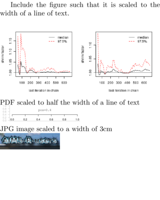
Include the figure such that it is scaled to
the width of a line of text.\\
\includegraphics[width=\linewidth]
{images/gelman1.png}\\
PDF scaled to half the width of a line of text\\
\includegraphics[width=0.5\linewidth]
{images/graphics-tut5_1-axisposPlot.pdf}\\
JPG image scaled to a width of 3cm\\
\includegraphics[width=3cm]
{../images/logo.jpg}\\
\end{document}
|
 |
| LaTeX code | PDF result |
|---|---|
  \documentclass{article}
  \usepackage{graphicx}
  \begin{document}
  Rotate the image 30 degrees and scale
  it to a width of 3cm (left figure)\\
  Scale the image to a width of 3cm and
  then rotate it by 30 degrees (right figure)\\
  \includegraphics[angle=30,width=3cm]
  {../images/logo.jpg}
  \includegraphics[width=3cm,angle=30]
  {../images/logo.jpg}\\
  Scale the image to 1.5 (50\% bigger)\\
  \includegraphics[scale=1.5]
  {../images/logo.jpg}\\
  \end{document}
|
 |
Vector graphics within LaTeX
As well as importing graphics from external sources, there is a very rich set of tools for generating scalable vector graphics within LaTeX. Arguably the most comprehensive of these toolsets is the PGF/Tikz tools.
The Portable Graphics Format (PGF) is actually a graphics layer and language for producing graphics. Tikz provides a syntax layer that sits on top of PGF making it easier to generate PGF syntax.
As this is a very substantial topic, PGF/Tikz will be the subject of a dedicated tutorial.
PGF/Tikz wikibook.Tables
Tables are relatively complex structures and there are a number of special table types (such as multi-page tables) that pose sufficient challenges to warrant equally specialized packages to facilitate their creation. Nevertheless, most table environments are variations on the tabular environment. Hence, we will start by exploring this environment.
The tabular environment
The tabular environment arranges content of each line (row) into columns, the widths of which are determined automatically. The tabular environment has the general form of:
  \begin{tabular}[pos]{table spec}
  ...
  \end{tabular}
The optional pos argument can be used to indicate the relative vertical alignment of the table relative to the baseline of the surrounding text and thus is only necessary when a table is to line up next to another table, graphic or text.
| Pos option | Description |
|---|---|
| b | Line the bottom of the table with the baseline of the surrounding text |
| c | Line the center of the table with the baseline of the surrounding text (default) |
| t | Line the top of the table with the baseline of the surrounding text |
The table spec argument defines the alignment of each column in the table. The widths of columns are automatically determined based on the contents of each column. However, tables cannot be wider than the width of a line of regular text, and thus over full content will be truncated. To fix the width of a column to a specific size and force the content to wrap (similar to regular paragraph text), the table spec argument also offers a special p{'width'} column specifier. The 'width' is any valid length measurement.
| Table spec option | Description |
|---|---|
| l | Left-justify the column content |
| c | Center the column content |
| r | Right-justify the column content |
| p{'width'} | Paragraph-like text wrapping of content |
| | | A vertical line separating the column |
| || | A double vertical line separating the column |
| @{.} | Separate columns with string between curly braces |
Within the table itself, the following control sequences are used:
| Control sequence | Description |
|---|---|
| & | Column separator |
| \\ | End of line marker. Indicates that a line break should be inserted |
| \hline | A horizontal line spanning the full width of the table |
| \cline{i-j} | A horizontal line spanning from the ith to the jth column |
Simple examples
| LaTeX code | PDF result |
|---|---|
  \documentclass{article}
  \begin{document}
  \begin{tabular}{lcr}
  \hline
  Column A&Column B&Column C\\
  \hline
  Category 1&High&100.00\\
  Category 2&High&80.50\\
  \hline
  \end{tabular}
  \end{document}
|
 |
| LaTeX code | PDF result |
|---|---|
  \documentclass{article}
  \begin{document}
  \begin{tabular}{l||c|r}
  \hline
  Column A&Column B&Column C\\
  \hline
  Category 1&High&100.00\\
  Category 2&High&80.50\\
  \hline
  \end{tabular}
  \end{document}
|
 |
| LaTeX code | PDF result |
|---|---|
  \documentclass{article}
  \begin{document}
  \begin{tabular}{lcr}
  \hline
  Column A&Column B&Column C\\
  \cline{2-3}
  Category 1&High&100.00\\
  Category 2&High&80.50\\
  \hline
  \end{tabular}
  \end{document}
|
 |
| LaTeX code | PDF result |
|---|---|
  \documentclass{article}
  \begin{document}
  \begin{tabular}{l||@{}c|@{\hspace{1.5cm}}r}
  \hline
  Column A&Column B&Column C\\
  \hline
  Category 1&High&100.00\\
  Category 2&High&80.50\\
  \hline
  \end{tabular}
  \end{document}
|
 |
Spanning
It is also possible to allow the content of a cell to span multiple columns or rows.Cells spanning multiple columns
Having a cell span multiple columns is achieved via the \multicolumn{cols}{alignment}{content} control sequence, where cols is the number of columns that the cell should span, alignment is one of the alignment values (l,c,r,p{}) from the tab spec above, and content is the content to be included in the cell.| LaTeX code | PDF result |
|---|---|
  \documentclass{article}
  \begin{document}
  \begin{tabular}{lcr}
  \hline
  &\multicolumn{2}{c}{Multi}\\\\
  \cline{2-3}
  Column A&Column B&Column C\\
  \hline
  Category 1&High&100.00\\
  Category 2&High&80.50\\
  \hline
  \end{tabular}
  \end{document}
|
 |
Cells spanning multiple rows
The ability to have content span multiple rows requires an additional package (multirow). This package must be declared in the preamble of the source document and then provides the \multirow{rows}{width}{content} control sequence, where rows is the number of rows that the cell should span, width is the width of the cell (* means use the natural width of the content), and content is the content to be included in the cell.| LaTeX code | PDF result |
|---|---|
  \documentclass{article}
  \\usepackage{multirow}
  \begin{document}
  \begin{tabular}{lcr}
  \hline
  Column A&Column B&Column C\\
  \hline
  \multirow{2}{*}{Category 1}&High&100.00\\
  &High&95.00\\
  \multirow{2}{*}{Category 2}&High&80.50\\
  &High&82.00\\
  \hline
  \end{tabular}
  \end{document}
|
 |
Hierarchical tables
Hierarchical tables (illustrated in the following example), are a way of displaying multiple tables together into a single table. There are two important considerations for producing hierarchical tables in LaTeX:- use \multicolumn{}{}{} to set the sub-table headings
- use \cline{} to put horizontal lines above the sub-table headings
- place an additional (empty) column between each of the sub-tables. This ensures a gap in the horizontal lines
| LaTeX code |
|---|
  \documentclass{article}
  \usepackage{multirow}
  \begin{document}
  \begin{document}
  \begin{tabular}{lrrrcrrr}
  \hline
  &\multicolumn{3}{c}{Winter}&&\multicolumn{3}{c}{Summer}\\
  \cline{2-4}\cline{6-8}
  Term&Slope&d.f.&P-value&&Slope&d.f.&P-value\\
  \hline
  A&1.24&22&0.011&&2.62&22&$<$0.001\\
   B&-3.87&23&0.026&&-2.28&23&0.001\\
   \hline
   \end{tabular}
   \end{document}
|
PDF result |
 |
Fixed column widths and text wrapping
| LaTeX code | PDF result |
|---|---|
  \documentclass{article}
  \begin{document}
  \\begin{tabular}{lcp{3cm}}
  \\hline
  Column A&Column B&Column C\\\\
  \\hline
  Category 1&High&A much larger block of text
  that would otherwise extend outside of the
  bounds of the page\\\\
  Category 2&High&This one is not so large\\\\
  \\hline
  \\end{tabular}
  \end{document}
|
 |
Colors in tables
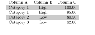
Colored backgrounds and borders in tables is provided by the xcolor package. This package needs to be loaded in the preamble and with the table optional argument.Colored table rows
The control sequence \rowcolors{first row}{odd color}{even color} pre-sets the color for odd and even rows. It should appear in the source document before the table.| LaTeX code | PDF result |
|---|---|
  \documentclass{article}
  \usepackage[table]{xcolor}
  \begin{document}
  \rowcolors{2}{white}{lightgray}
  \begin{tabular}{lcr}
  \hline
  Column A&Column B&Column C\\
  \hline
  Category 1&High&100.00\\
  Category 1&High&95.00\\
  Category 2&Low&80.50\\
  Category 3&Low&82.00\\
  \hline
  \end{tabular}
  \end{document}
|
 |
There are two switches switch row coloring on and off:
- \hiderowcolors - hide the coloring of rows from this point on
- \showrowcolors - show the coloring of rows from this point on
Colors of individual cells
| LaTeX code | PDF result |
|---|---|
  \documentclass{article}
  \usepackage[table]{xcolor}
  \begin{document}
  \rowcolors{2}{white}{lightgray}
  \begin{tabular}{lcr}
  \hline
  Column A&Column B&Column C\\
  \hline
  Category 1&High&100.00\\
  Category 1&High&95.00\\
  Category 2&Low&80.50\\
  Category 3&Low&82.00\\
  \hline
  \end{tabular}
  \end{document}
|
 |
Customizations
Most of the formatting rules used to set out a table are stored in variables and thus, by altering these variables, it is possible to tweak/alter the appearance of tables. The following table provides the most common of these.| Variable | Example | Description |
|---|---|---|
| \tabcolsep | \setlength{\tabcolsep}{5pt} | Set the amount of space between columns to be 5pt |
| \arraystretch | \renewcommmand{\arraystretch}{1.5} | Set the amount of space between rows to be 1.5 lines |
The tabularx package
The width of regular tables is determined by the table content. For many tables, this is sufficient. However, when there are many columns and/or large amounts of content, the tables can extend beyond the edges of the page.
The tabularx package (which as a package must be loaded in the preamble) extends the functionality of table creation to allow you to indicate the total width of the table. This new environment, builds on the regular tabular environment. To enable content to fit within a fixed width table, the tabularx introduces a new table spec (X) that indicates that the width of the column is to stretched to allow the table to be the specified width.
The width of the table is defined by an optional length argument to the tabularx environment.
The X column specifier is replaced by a p{} and the width is worked out automatically. If multiple X column specifiers are supplied, then the stretched space will be evenly distributed between all of these columns. Hence, the tabularx environment also makes a simple way to create a table with equal width columns irrespective of their content.
| LaTeX code | PDF result |
|---|---|
  \documentclass{article}
  \usepackage{tabularx}
  \begin{document}
  \begin{tabularx}{\textwidth}{lXX}
  \hline
  Column A&Column B&Column C\\
  \hline
  Category 1&High&100.00\\
  Category 2&High&80.50\\
  \hline
  \end{tabularx}
  \end{document}
|
 |
In order to alter the justification within a stretched column, you can use the \newcolumntype{name}{format} control sequence (in the array package), where name is a single letter name for a new column specifier and format provides the format of this new specifier.
In the following example, the second and third columns are stretched to make the table equal to 90% of the width of a regular line of text. The second column is center justified and the third column is right justified.
| LaTeX code |
|---|
  \documentclass{article}
  \usepackage{tabularx}
  \usepackage{array}
  \begin{document}
  \newcolumntype{C}{>{\centering\arraybackslash}X}%
  \newcolumntype{R}{>{\raggedleft\arraybackslash}X}%
  \begin{tabularx}{0.9\textwidth}{lCR}
  \hline
  Column A&Column B&Column C\\
  \hline
  Category 1&High&100.00\\
  Category 2&High&80.50\\
  \hline
  \end{tabularx}
  \end{document}
|
PDF result |
 |
In the above example, the second and third columns have equal widths. However, we can modify the definition of a new column specifier to include an argument that determines the fraction of total stretched width for each of the new columns. When doing so, the fractions used must add up to the total number of stretched columns (2 in the following example).
| LaTeX code |
|---|
  \documentclass{article}
  \usepackage{tabularx}
  \usepackage{array}
  \begin{document}
  \newcolumntype{C}[1]{>{\hsize=#1\hsize\centering\arraybackslash}X}%
  \newcolumntype{R}[1]{>{\hsize=#1\hsize\raggedleft\arraybackslash}X}%
  \begin{tabularx}{0.9\textwidth}{|l|C{0.5}|R{1.5}|}
  \hline
  Column A&Column B&Column C\\
  \hline
  Category 1&High&100.00\\
  Category 2&High&80.50\\
  \hline
  \end{tabularx}
  \end{document}
|
PDF result |
 |
The tabulary environment
The tabulary environment works similar to the tabularx package, except that it is capable of generating appropriate column widths so as to achieve equal row heights. Moreover, unlike the tabularx environment, the optional table width argument is taken as a maximum (rather than a fixed setting). This means that tables will be created to a maximum width, yet can be narrower if there is little content.
| LaTeX code | PDF result |
|---|---|
  \documentclass{article}
  \usepackage{tabulary}
  \begin{document}
  \begin{tabulary}{0.7\textwidth}{JCR}
  \hline
  Category&Temperature&Response\\
  \hline
  1&High and sometimes low&100.00\\
  2&High&80.50\\
  \hline
  \end{tabulary}
  \end{document}
|
 |
The tabu environment
The tabu package provides the tabu environment which works similar to the tabularx environment. As well as allowing stretchy columns for fixed table widths, the tabu environment handles multi-page tables and footnotes.
Multi-page tables
Occasionally a table contains too many rows to fit on a single page. For such circumstances, there is the longtable environment of the longtable package. This environment operates similar to the regular tabular environment except that it can split the content across multiple pages.When splitting across pages, different tables and headers can be defined for the last and first pages respectively. This allows for running headers and footers and is achieved via the following switches.
| Switch | Description |
|---|---|
| \endfirsthead | Indicates that the definition for the header for the first page is complete |
| \endhead | Indicates that the definition for the header for subsequent pages is complete |
| \endfoot | Indicates that the definition for the footer for all pages (except the last) is complete |
| \endlastfoot | Indicates that the definition for the footer for the last page complete |
| LaTeX code |
|---|
  \documentclass{article}
  \usepackage{longtable}
  \begin{document}
  \begin{longtable}{lcr}

  \hline
  Category&Temperature&Response\\
  \hline
  \endfirsthead

  \multicolumn{3}{r}{\tablename~\thetable{} -- continued}\\
  \hline
  Category&Temperature&Response\\
  \hline
  \endhead

  \hline
  \multicolumn{3}{r}{continued on next page}\\
  \hline
  \endfoot

  \hline
  \endlastfoot

  1&High&100.00\\
  2&High&80.50\\
  1&High&95.00\\
  2&High&83.00\\
  1&Medium&120.00\\
  2&Medium&90.50\\
  1&Medium&130.50\\
  2&Medium&88.50\\
  1&Low&200.00\\
  2&Low&180.00\\
  1&Low&220.00\\
  2&Low&170.00\\
  \end{longtable}
  \end{document}
|
PDF result |
  |
The booktabs package
The booktabs package provides numerous additional control sequences and switches to use in the various table environments to help in the production of more professional looking tables. The following table provides a summary of those additional control sequences.
| Switch | Description |
|---|---|
| \toprule | Specifies a thick horizontal line (appropriate for the top of a table). |
| \midrule | Specifies a normal thickness horizontal line (appropriate for the end of the header of a table). |
| \bottomrule | Specifies a thick horizontal line (appropriate for the bottom of a table). |
| \cmidrule | Specifies a mid thickness horizontal line equivalent to a \cline{}. |
| LaTeX code | PDF result |
|---|---|
  \documentclass{article}
  \usepackage{tabulary}
  \begin{document}
  \usepackage{booktabs}
  \begin{document}
  \begin{tabular}{lcr}
  \toprule
  Category&Temperature&Response\\
  \midrule
  1&High&100.00\\
  2&High&80.50\\
  \bottomrule
  \end{tabular}
  \end{document}
|
 |
Floating environments
Floats are containers for content that cannot be split over multiple pages (such as figures and tables). Rather than being set in the location in which they appear in the source document (which may not provide sufficient space before the end of the page), floats reserve a space in one of a number of predefined regions within either the current or a later page for the content.Floats are ideal containers for content such as figures or tables and indeed the two most common float environments are:
- figure
- table
Floats take on the general form of:
  \begin{float}[placement specifier]
  ...
  \end{float}
where float is the name of the floating environment. placement specifier is
a specifier indicating a preference for where the float should appear within a page.
The placement specifier is only a preference and therefore may be ignored if the preferred placement violates the typical page and paragraph layout rules. For example, a float would not be placed in a place in text that would result in a paragraph being broken in half.
As this is a preference list, multiple placement values can be specified and LaTeX will go through each of the placements in order in an attempt to find a float placement that meets your highest preference whilst still maintaining document flow.
| Placement specifier | Description |
|---|---|
| h | Place the float here (approximately where it appears in the source document) |
| t | Place the float at the top of the page (this or subsequent) |
| b | Place the float at the bottom of the page (this or subsequent) |
| p | Place the float on a separate page reserved for floats |
| ! | Override some of the rules used by LaTeX in determining float placement whilst maintaining document flow. The ! forces the placement specifier to be honored exactly. |
Captions
Table and figure floating environments both support captioning via a control sequence called \caption[short caption]{full caption}. LaTeX assigns a separate counter for each floating environment type and automatically handles the labeling and numbering of floats.The full caption, including the label (Table or Figure) and numbering will be placed within the float in the location that the \caption{} control sequence appears relative to the rest of the content. For example, if \caption{} appears at the start of the floating environment, then the caption will appear at the top of the float (above the content), if \caption{} is at the end of the floating environment, then the caption will be underneath the content.
The optional parameter to the \caption[]{} control sequence specifies a shorter caption. This shorter caption (if provided) is used when constructing a list of figures or tables.
Whilst the caption will be centered within the floating environment, the content will be left justified. Hence, it is common wrap the content within a center environment.
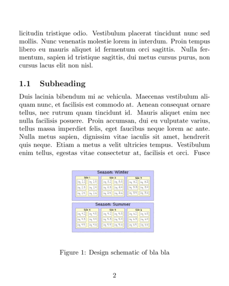
Floating figures
Try to float a graphic and its caption at the approximate location that it appears in the source document (h), if not, try putting it at the top of the next page (t), if not the bottom b or as a last resort, on a dedicated float page (p). I have included a partial code snippet, just displaying the syntax relevant for the floating figure.
 \documentclass{article}
 ...
 \usepackage{graphicx}
 \begin{document}
 ...
 \begin{figure}[htbp]
 \includegraphics{images/ws9.2aQ1.1.png}\\
 \caption{Design schematic of bla bla}
 \end{figure}
 ...
 \end{document}
 |
 |
Notice in the example above, that the figure caption is centered whereas the graphic is not. We will address this in the next example.
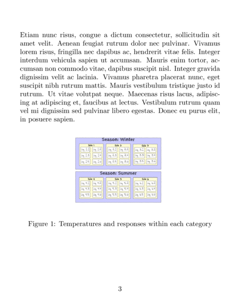
Force the floating figure to be placed at the bottom (!b) of the page (next in this case). and center the graphic within this float. Again, I have included a partial code snippet, just displaying the syntax relevant for the floating figure.
 \documentclass{article}
 ...
 \usepackage{graphicx}
 \begin{document}
 ...
 \begin{figure}[!b]
 \begin{center}
 \includegraphics[width=0.5\\linewidth]{images/ws9.2aQ1.1.png}\\
 \end{center}
 \caption{Design schematic of bla bla}
 \end{figure}
 ...
 \end{document}
 |
 |
List of figures and tables
For longer documents such as books, long reports and theses, lists of tables and figures provide useful ways of looking up information. These lists are somewhat similar to a table of contents and are typically placed straight after the table of contents.
 \documentclass{article}
 ...
 \usepackage{graphicx}
 \usepackage{booktabs}
 \begin{document}
 ...
 \begin{table}[htbp]
 \begin{center}
 \caption{Design schematic of bla bla}
 \begin{tabular}{lcr}
 \toprule
 Category&Temperature&Response\\
 \midrule
 1&High&100.00\\
 2&High&80.50\\
 \bottomrule
 \end{tabular}
 \end{center}
 \end{table}
 ...
 \begin{figure}[!b]
 \begin{center}
 \includegraphics[width=0.5\\linewidth]{images/ws9.2aQ1.1.png}\\
 \end{center}
 \caption{Temperatures and responses within each category}
 \end{figure}
 ...
 \end{document}
 |
 |
 |
 |
Referencing
Many elements in LaTeX have associated counters to keep track of numbering. For example, there are counters for sectioning, tables, figures, formulae etc. It is possible to associate labels with any of these elements.As the source document is being processed, the value of the counter for the element to which the label is attached, as well as the page number are stored in an axillary file. The counter values and page numbers can then be referenced from another point in the document. That is, they allow elements to be referred to.
The following table documents the most important control sequences for referencing. Each of these take a common compulsory parameter - a unique marker or identifier. The marker can be any string of characters, yet it many find it useful to begin the string with a prefix that represents the sort of element being referenced ( such as sec: for section, fig: for figure etc).
| Control sequences | Example | Description |
|---|---|---|
| \label{marker} | \label{sec:introduction} | Define a label to the introduction section |
| \ref{marker} | \ref{sec:introduction} | Refer to the element whose label is sec:introduction |
| \pageref{marker} | \pageref{sec:introduction} | The page number for the page containing the element whose label is sec:introduction |
Examples
 \documentclass{article}
 ...
 \usepackage{graphicx}
 \usepackage{booktabs}
 \begin{document}
 \section{Introduction}\label{sec:introduction}
 This is some text that refers to table~\ref{tab:schematic}
 \begin{table}[htbp]
 \begin{center}
 \caption[Design schematic of seasonal experiment]{Design schematic of seasonal experiment}
 \label{tab:schematic}
 \begin{tabular}{lcr}
 \toprule
 Category&Temperature&Response\\
 \midrule
 1&High&100.00\\
 2&High&80.50\\
 \bottomrule
 \end{tabular}
 \end{center}
 \end{table}
 \subsection{Subheading}
 Here is some more text.  This sentence refers to section~\ref{sec:introduction} on
 page~\pageref{sec:introduction}
 \end{document}
| *.aux file | PDF file |
|---|---|
  ...
  \newlabel{sec:introduction}{{1}{1}}
  ...
  \newlabel{tab:schematic}{{1}{1}}
  ...
The first {1} is the value of the element counter.
The second {1} is the page number.
|
 |
Footnotes
Footnotes are a convenient way to provide extra information or clarification without compromising conciseness or derailing the progression of ideas. Typically, subscript numbers are placed in the main text to indicate a place where a footnote is required and footnotes (the additional information) are set in a smaller font at the bottom of the page.
In LaTeX, footnotes are automatically handled via the \footnote{} control sequence. The single compulsory parameter is the text to place in the footnote at the bottom of the page.
| LaTeX code | PDF result |
|---|---|
  \documentclass{article}
  \begin{document}
  \begin{document}
  There is a counter associated with
  footnotes and the footnote mark number
  increments throughout the
  document\footnote{footnotes can be
  customized to allow the footnote marker
  number resets each page.}
  \end{document}
|
 |
Bibliographies
In academic writing it is important to cite the original source of information and ideas. Not only does this provide due credit to the author(s) of those data and ideas, it also allows the reader the opportunity to independently evaluate the quality and context of the information and data.
Whilst it is possible to manually enter, format and manage each of the cited works in your LaTeX source document as if it were any other text, different journals and audiences require different formatting styles for both in text citations as well as the list of references at the end of the document. Hence, altering the styles to accommodate different audiences can be time consuming and error prone. Moreover, major edits of the main text body then require careful scrutiny in order to ensure all in-text citations are correctly formatted (i.e. there are often rules about the order of multiple references grouped together, some styles dictate different formats for the first time a piece of work is cited in the document compared to subsequent citations) and that in-text citations match up with the reference list.
In LaTeX, bibliographies are handled by an external application, BibTeX, which is included in most TeX distributions. Along with a bibliography rendering engine, BibTeX defines a flat-text bibliography database (*.bib) for the storage of references.
BibTeX database
In keeping with the simple plain text nature of LaTeX source files, BibTeX files (*.bib) are also simple plain text. The general structure of BibTeX entries is exemplified as follows (two examples, one of an article and the other of a book):
  @article{Bolker-2008-127,
  author = {Bolker, B. M. and Brooks, M. E. and Clark, C. J. and Geange, S. W. and Poulsen,
  J. R. and Stevens, H. H. and White, J. S.},
  journal = {Trends in Ecology and Evolution},
  number = {3},
  pages = {127-135},
  title = {Generalized linear mixed models: a practical guide for ecology and evolution},
  volume = {24},
  year = {2008}
  }

  @book{goossens93,
  author    = "Michel Goossens and Frank Mittlebach and Alexander Samarin",
  title     = "The LaTeX Companion",
  year      = "1993",
  publisher = "Addison-Wesley",
  address   = "Reading, Massachusetts"
  }
- Entries begin with a declaration of the type of reference (e.g. article, book etc).
- The main body of an entry comprises a number of reference attributes (such as the authors, title, year published etc), each represented as a name = value pair and separated by commas
- The first attribute is a unique identifier for the entry. Whilst this can be any unique combination of characters, experienced users tend to settle on a format that reflects the actual reference (such as a combination of first author and year/page number etc)
- The value must be enclosed in either double quotation marks ("") or curly braces ({})
- Depending on the reference type, some attributes are compulsory and others are optional and the order of the attributes is unimportant.
- Accented and other special characters are supported as in LaTeX.
- Authors values can be specified as either surname, forename or forename surname
- Multiple authors are separated by an and
| Reference type | Description | Example |
|---|---|---|
| @article | journal or magazine article |
  @article{authorYear,
  author    = {},
  title     = {},
  journal   = {},
  %volume   = {},
  %number   = {},
  %pages    = {},
  year      = {XXXX},
  %month    = {},
  %note     = {},
  }
|
| @book | Published book |
  @book{authorYear,
  author    = {},
  title     = {},
  publisher = {},
  %volume   = {},
  %number   = {},
  %series   = {},
  %address  = {},
  %edition  = {},
  year      = {XXXX},
  %month    = {},
  %note     = {},
  }
|
| @incollection | A chapter in a book |
  @incollection{authorYear,
  author    = {},
  title     = {},
  booktitle = {},
  publisher = {},
  %editor   = {},
  %volume   = {},
  %number   = {},
  %series   = {},
  %type     = {},
  %chapter  = {},
  %pages    = {},
  %address  = {},
  %edition  = {},
  year      = {XXXX},
  %month    = {},
  %note     = {},
  }
|
| @inproceedings and @conference | An article in conference proceedings |
  @inproceedings{authorYear,
  author        = {},
  title         = {},
  booktitle     = {},
  %editor       = {},
  %volume       = {},
  %number       = {},
  %series       = {},
  %pages        = {},
  %address      = {},
  %organization = {},
  %publisher    = {},
  year          = {XXXX},
  %month        = {},
  %note         = {},
  }
|
| @manual | A reference manual for software or R package |
  @manual{authorYear,
  %author        = {},
  title         = {},
  %organization = {},
  %address      = {},
  %edition     = {},
  %year          = {XXXX},
  %month        = {},
  %note         = {},
  }
|
| @techreport | A report (grey literature) |
  @techreport{authorYear,
  author      = {},
  title       = {},
  institution = {},
  %type       = {},
  %number     = {},
  %address    = {},
  year        = {XXXX},
  %month      = {},
  %note       = {},
  }
|
| @mastersthesis | A Master's thesis |
  @mastersthesis{authorYear,
  author      = {},
  title       = {},
  school      = {},
  %type       = {},
  %address    = {},
  year        = {XXXX},
  %month      = {},
  %note       = {},
  }
|
| @phdthesis | A Ph.D. thesis |
  @phdthesis{authorYear,
  author       = {},
  title        = {},
  school       = {},
  %type        = {},
  %address     = {},
  howpublished = {},
  year         = {XXXX},
  %month       = {},
  %note        = {},
  }
|
| @proceedings | Conference proceedings |
  @proceedings{authorYear,
  title         = {},
  school        = {},
  %editor       = {},
  %volume       = {},
  %number       = {},
  %series       = {},
  %organization = {},
  %publisher    = {},
  %address      = {},
  year          = {XXXX},
  %month        = {},
  %note         = {},
  }
|
| @inbook | A section of a book, yet one that does not have its own title |
  @inbook{authorYear,
  title         = {},
  author        = {},
  school        = {},
  chapter       = {},
  pages         = {},
  publisher     = {},
  %editor       = {},
  %volume       = {},
  %number       = {},
  %series       = {},
  %type         = {},
  %address      = {},
  %edition      = {},
  year          = {XXXX},
  %month        = {},
  %note         = {},
  }
|
| @misc | All other types of publications - such as a website |
  @misc{authorYear,
  %title        = {},
  %author       = {},
  %howpublished = {},
  school        = {},
  chapter       = {},
  pages         = {},
  publisher     = {},
  year          = {XXXX},
  %month        = {},
  %note         = {},
  }
|
| Attribute | Description |
|---|---|
| address | The publishers address - typically just the city |
| author | The author(s) names |
| booktitle | Title of the conference proceedings of book |
| chapter | The chapter number |
| edition | Edition of the book (e.g. "First") |
| editor | The editor(s) names |
| howpublished | The method of publishing - if non standard |
| institution | The name of the institution from which the work originated |
| journal | The name of the journal |
| month | The name of the month of publication or creation or release |
| note | Miscellaneous extra notes |
| number | The issue number of the publication |
| organization | The name of the conference sponsor |
| pages | The range of pages over which the work occurs |
| publisher | The name of the publisher |
| school | The school in which the thesis was submitted |
| series | The series in which the book is published |
| title | The title of the work |
| type | The type of publication |
| url | Web address |
| volume | The volume of the publication |
| year | The year of the publication |
BibTeX
LaTeX and BibTex work together to embed citations and a list of references into the final document. Where citations are required, a special control sequence (\cite{}) is added. This control sequence has a single parameter - the unique identify of a reference in a BibTeX database file.In addition to these citation markers, the source document should contain two additional control sequences at the end of the document (yet prior to the \end{document} marker):
- \bibliographystyle{} - this indicates the style of the bibliography. We return to this later.
- \bibliography{} - this points to one or more BibTeX database files. It also serves to indicate where the list of references should be placed in the final document.
| LaTeX source file (for example tut17.1S13.1a.tex) |
|---|
  \documentclass{article}
  \begin{document}
  ... a easily digestible treatment of generalized linear
  mixed effects models \cite{Bolker-2008-127}.
  \bibliographystyle{plain}
  \bibliography{refs.bib}
  \end{document}
|
BibTeX database file (for example refs.bib) |
  @article{Bolker-2008-127,
  author = {Bolker, B. M. and Brooks, M. E. and Clark, C. J. and Geange, S. W. and Poulsen,
  J. R. and Stevens, H. H. and White, J. S.},
  journal = {Trends in Ecology and Evolution},
  number = {3},
  pages = {127-135},
  title = {Generalized linear mixed models: a practical guide for ecology and evolution},
  volume = {24},
  year = {2008}
  }

  @book{goossens93,
  author    = "Michel Goossens and Frank Mittlebach and Alexander Samarin",
  title     = "The LaTeX Companion",
  year      = "1993",
  publisher = "Addison-Wesley",
  address   = "Reading, Massachusetts"
  }
|
- Firstly, as the LaTeX engine processes the source document and when it encounters one of the citation control sequences (see below) an
entry is written to the *.aux axillary file.
xelatex tut17.1S13.1a.tex
At this stage (prior to running BibTeX, LaTeX is unable to resolve the citation and thus inserts a ?.LaTeX axillary file (for example tut17.1S13.1a.aux) PDF output \relax \citation{Bolker-2008-127} \bibstyle{plain} \bibdata{refs.bib}
- When BibTex is then run on this *.aux file:
bibtex tut17.1S13.1a.aux
Essentially, BibTeX determines which of the references in the *.bib file are required (based on what entries are in the *.aux file, and then formats the references according to the nominated bibliography style. This information is collected together into an environment and awaits an additional LaTeX run when it will be incorporated into the document at runtime.BibTeX library file (for example tut17.1S13.1a.bbl) \begin{thebibliography}{1} \bibitem{Bolker-2008-127} B.~M. Bolker, M.~E. Brooks, C.~J. Clark, S.~W. Geange, J.~R. Poulsen, H.~H. Stevens, and J.~S. White. \newblock Generalized linear mixed models: a practical guide for ecology and evolution. \newblock {\em Trends in Ecology and Evolution}, 24(3):127--135, 2008. \end{thebibliography}BibTeX also modifies the *.aux file. It adds a \bibcite{}{} control sequence for each of the cited references. These control sequences indicate the format of the in-text citation.
- When LaTeX is run for a second time, the *.bbl file is parsed during the source document
preamble, and therefore, the references are now available for inclusion.
xelatex tut17.1S13.1a.tex

- Finally, we run LaTeX a third time to ensure that all the citation information has been included in the
the document.
xelatex tut17.1S13.1a.tex

Bibliography (list of references) styles
There is not a single referencing format. Different disciplines often require very different styles. Even within disciplines, formats can vary subtly or even substantially between journals. For example, some publications require that the list of references be ordered alphabetically by senior order, whilst others are sorted according to the order in which the works are cited in the main text.
The formatting of the bibliography (list of references) can be controlled by the \bibliographystyle{} control sequence. This takes a single parameter, the name (including full path if not one of the pre-installed styles).
| Style | Reference Key | Reference author format | Reference sorting | Citation style |
|---|---|---|---|---|
| plain | Unique number | Michael Goossens | by author | Numbers in brackets |
| unsrt | Unique number | Michael Goossens | in-text citing order | Numbers in brackets |
| abbrv | Unique number | M. Goossens | by author | Numbers in brackets |
| ieeetr | Unique number | M. Goossens | by author | Numbers in brackets |
| acm | Unique number | GOOSSENS, M. | by author | Numbers in brackets |
| siam | Unique number | GOOSSENS, M. | by author | Numbers in brackets |
| alpha | Abbreviated author/year | Michael Goossens | by author | GMS93 |
| ieetr | Unique number | M. Goossens | in-text citation order | Goossens et. al., 1993 |
| apalike | Author/year | Goossens, M. | by author | Goossens et. al., 1993 |
- LaTeX and BibTeX style files for biologists
- Bibliography style files for selected ecology/biology journals
 \documentclass{article}
 \begin{document}
 ... a easily digestible treatment of generalized linear
 mixed effects models \cite{goossens93,Bolker-2008-127}.
 \bibliographystyle{apalike}
 \bibliography{References/refs.bib}
 \end{document}

In addition to the bibliography style files that come with modern TeX distributions, it is possible to modify these to create new styles that meet your needs. Moreover, many publishers also make bibliography style files available to authors support their referencing requirements. These bibliography style files can either be placed in the same directory as the original *.tex source document, or, if placed in another directory, the \bibliographystyle style parameter must include the full path name.
The next section introduces a package for supporting even further bibliography styles.
In-text citations
The stock standard citation style in LaTeX/BibTeX is to use numbers to distinguish citations (see example above). Whilst this is indeed the format adopted by some journals, other journals use various forms of the author-year citation style.The natbib package provides a great flexibility of in-text citation styles. In order to use the following in-text citation styles, you must first make two alterations to the source document:
- Use the package in the source preamble:
\usepackage[options]{natbib}Options Description authoryear Author/year citation style (default for natbib) numbers Numeric citation style (default for non natbib) super Superscripted numeric citation style colon Multiple citations separated by colons (default for natbib) comma Multiple citations separated by commas sort Multiple citations are ordered according to their order in the reference section. sort&compress As for sort, also compressing multiple citations longnamesfirst The first occurrence a multi-author citation including expanded author list, subsequent occurrences using an abbreviated style (e.g. et. al.) round Parentheses () (default for natbib) square Square brackets [] curly Curly braces {} angle Angle brackets <> - Alter the bibliography style to one of the natbib compatible styles (see table below):
\bibliographystyle{style}Styles Description plainnat Natbib compatible version of the plain bibliography style abbrvnat Natbib compatible version of the abbrv bibliography style unsrtnat Natbib compatible version of the unsrt bibliography style
| Control sequence | Citation style example |
|---|---|
| \citet{Bolker-2008-127} | Bolker et. al. (2008) |
| \citep{Bolker-2008-127} | (Bolker et. al, 2008) |
| \citet*{Bolker-2008-127} | Bolker, Brooks, Clark, Geange, Poulson, Stevens and White (2008) |
| \citep*{Bolker-2008-127} | (Bolker, Brooks, Clark, Geange, Poulson, Stevens and White, 2008) |
| \citeauthor{Bolker-2008-127} | Bolker et. al. |
| \citeauthor*{Bolker-2008-127} | Bolker, Brooks, Clark, Geange, Poulson, Stevens and White |
| \citeyear{Bolker-2008-127} | 2008 |
| \citeyearpar{Bolker-2008-127} | (2008) |
| \citealt{Bolker-2008-127} | Bolker et. al. 2008 |
| \citealp{Bolker-2008-127} | Bolker et. al, 2008 |
| \citetext{pers.\ comm.} | (pers. comm.) |
 \documentclass{article}
 \usepackage[round]{natbib}
 \begin{document}
 ... a easily digestible treatment of generalized linear
 mixed effects models \cite{Bolker-2008-127}.
 Multiple references will appear in the order that they are provided \citep{Bolker-2008-127,goossens93},
 unless the sort option is used.
 \bibliographystyle{apalike}
 \bibliography{References/refs.bib}
 \end{document}

Mathematical formulae
As mentioned in the introduction to this tutorial, one of the greatest motivating factors in the development of TeX, was the need to produce elegant mathematical equations. Testament to the success of this component is the fact that this mathematical engine has become the benchmark by which all other equation generators are compared. Indeed, many other applications adopt the LaTeX math engine for equations.
LaTeX typesets mathematical notation differently (has different rules etc) than regular text. Therefore all mathematical notation must occur within dedicated math environments.
Mathematical environments
Mathematical equations can occur either:- inline - surrounded by regular text without line. Typically, inline equations are just for very simple equations that lack complex symbols and structures that do not disrupt the usual spacing of lines of text.
- displayed - separated from the main text.
| Environment | TeX shorthand | LaTeX shorthand |
|---|---|---|
| math | \(..\) | $..$ |
| displaymath | \[..\] | $$..$$ |
| LaTeX code | PDF result |
|---|---|
  \documentclass{article}
  \begin{document}
  The formula, $y=mx+c$, is displayed inline.
  Some symbols and equations (such as
  $\sum{x}$ or $\frac{1}{2}$) are rescaled
  to prevent disruptions to the regular
  line spacing.
  For more voluminous equations (such as
  $\sum{\\frac{(\mu - \bar{x})^2}{n-1}}$),
  some line spacing disruptions are unavoidable.
  Math should then be displayed in displayed mode.
  $$\sum{\frac{(\mu - \bar{x})^2}{n-1}}$$
  \end{document}
|
 |
There are some additional considerations while in math mode (the mode used to typeset mathematical equations either inline or displayed) compared to regular text mode:
- Each letter is considered to represent a separate variable and is therefore italicized. In order to preserve the regular text style of words within formulae, the word must be used as an argument to a \text{} control sequence.
- Most spaces (including those between words as math mode does not recognize words) are ignored in math mode. Additional space within formulae can be defined with the \quad and \qquad control sequences (see below)
- Blank lines are not permitted within math mode
Symbols
Within math mode, the following symbols have their usual meaning:+ - = ! / ( ) [ ] < > | ' :However, for all other symbols (including operators, Greek letters, delimiters as well as set and logic notation), special control sequences exist. The list of available symbols within base LaTeX and through packages is huge and finding the appropriate control sequences for the required symbol can be a daunting task. Two resources however, greatly alleviate these pains:
- symbols-a4.pdf - a PDF document
- Detetify - LaTeX symbol classifier - an ingenious web tool that provides a list of candidate symbols based on a scribbled symbol you have drawn on its canvas.
Operators
|
|
Greek letters
|
|
Delimeters
|
Set and logic notation
|
|
Powers, indicies, and roots
| Symbol | Control sequence |
|---|---|
| $x^2$ $e^{x+1}$ | x^2 e^{x+1} |
| $x_2$ $x_{n+1}$ | x_2 x_{n+1} |
| $\sqrt{x}$ $\sqrt[3]{x}$ | \sqrt{x} \sqrt[3]{x} |
Sums and integrals
Sums and integrals are supported via the \sum{} and \int{} symbols respectively. Both of these symbols can receive carrot (^) and underscore (_) parameters to represent limits. Alternatively, for limits placed above and below the symbol, there is the \limits control sequence.| Example math code | Result |
|---|---|
$\sum x$. | $\sum x$ |
$\sum_{i=1}^{100} x$. | $\sum_{i=1}^{100} x$ |
$\sum\limits_{i=1}^{100} x$. | $\sum\limits_{i=1}^{100} x$ |
$\int_{0}^{\infty} e^{-x} dx$. | $\int_{0}^{\infty} e^{-x} dx$ |
$\int\limits_{0}^{\infty} e^{-x} dx$. | $\int\limits_{0}^{\infty} e^{-x} dx$ |
Fractions
| Example math code | Result |
|---|---|
The fraction was $4/5$. | The fraction was $4/5$ |
The fraction was $^4/_5$. | The fraction was $^4/_5$ |
$$\frac{x}{n-1}$$ | $$\frac{x}{n-1}$$ |
$$\frac{\sum{(x-\bar{x})^2}}{n-1}$$ | $$\frac{\sum{(x-\bar{x})^2}}{n-1}$$ |
Bracket and brace sizing
The brackets and braces listed in the table above all produce brackets and braces of a size appropriate to the current font size. However, when brackets or braces are supposed to surround larger content (or are nested within each other), it is necessary to use larger versions. This can be achieved either:- automatically - using the \left, \right and middle temporary command switches. When placed directly before one of the delimiters, it attempts to scales the delimiter according to the size of the adjoining content.
Example math code Result $$\left(\frac{x_2}{n-1}\right)$$$$\left(\frac{x_2}{n-1}\right)$$ $$\left\{\frac{x^2}{y^3}\right\}$$$$\left\{\frac{x^2}{y^3}\right\}$$ - manually - using the \big, \Big, \bigg, \Bigg modifier commands that define increasingly larger sizes that are particularly useful for nested brackets/braces.
Example math code Result $$\Big((x-\bar{x})^2 + (y-\bar{y})^2\Big)$$$$\Big((x-\bar{x})^2 + (y-\bar{y})^2\Big)$$
Mixing regular text and math
As mentioned previously, all letters are italicized and spaces are ignored. Nevertheless, it is possible to force the math engine to respect some text mode formatting via the \text{} control sequence. In addition, the other text formatting control sequences (\textrm{}, \textit{}, \textbf{} etc) can also be used.
| Example math code | Result |
|---|---|
$$response = constant + \beta \times IV1$$ | $$response = constant + \beta \times IV1$$ |
$$\text{response} = \text{constant} + \beta\times \text{IV1}$$ | $$\text{response} = \text{constant} + \beta\times \text{IV1}$$ |
$$\text{response} = \text{constant} + \beta\times \textbf{IV1}$$ | $$\text{response} = \text{constant} + \beta\times \textbf{IV1}$$ |
Formatting math font
Mathematics are often set in specific types of fonts (that differ from those fonts used in the main text). These alterations are available via the amsfonts package. The following table illustrates the various font styles available in math mode (when using the amsfonts package.| Math font control sequence | Sample | Use |
|---|---|---|
| \mathnormal{} |
 |
Typical mathematical notation (and default) |
| \mathrm{} |
 |
Appropriate for units of measurement or single word functions |
| \mathit{} |
 |
|
| \mathbf{} |
 |
Vector notation |
| \mathsf{} |
 |
|
| \mathtt{} |
 |
Monospace font to represent code |
| \mathcal{} |
 |
Calligraphy font to represent schemes and sheaves in number theory and algebraic geometry |
| \mathfrak{} |
 |
Fraktur font to represent lie algebras |
| \mathbb{} |
 |
Blackboard bold font to represent sets |
Accents in math mode
| Example math code | Result |
|---|---|
$a'$ $a''$ $a'''$ $a''''$ | $a'$ $a''$ $a'''$ $a''''$ |
$\underline{x}$ $\bar{x}$ | $\underline{x}$ $\bar{x}$ |
$\grave{x}$ $\acute{x}$ | $\grave{x}$ $\acute{x}$ |
$\dot{x}$ $\ddot{x}$ | $\dot{x}$ $\ddot{x}$ |
$\not{x}$ $\mathring{x}$ | $\not{x}$ $\mathring{x}$ |
$\overrightarrow{XY}$ $\overleftarrow{XY}$ | $\overrightarrow{XY}$ $\overleftarrow{XY}$ |
$\overline{x}$ $\vec{x}$ | $\overline{x}$ $\vec{x}$ |
$\check{x}$ $\breve{x}$ | $\check{x}$ $\breve{x}$ |
$\hat{x}$ $\widehat{XY}$ | $\hat{x}$ $\widehat{XY}$ |
$\tilde{x}$ $\widetilde{XY}$ | $\tilde{x}$ $\widetilde{XY}$ |
Horizontal spacing
As I have mentioned a couple of times, white space is largely ignored in math mode. There are a number of control sequences available for providing set amounts of horizontal space.| Control sequence | Example math code | Result | Description |
|---|---|---|---|
| \quad | $y=bx+a\quad\epsilon\sim{}N(0,1)$ | $y=bx+a\quad\epsilon\sim{}N(0,1)$ | A space equal to the font size |
| \qquad | $y=bx+a\qquad\epsilon\sim{}N(0,1)$ | $y=bx+a\qquad\epsilon\sim{}N(0,1)$ | A space twice that of the font size |
| \, | $y=bx+a\,\epsilon\sim{}N(0,1)$ | $y=bx+a\,\epsilon\sim{}N(0,1)$ | Small space (3/18 of a quad) |
| \: | $y=bx+a\:\epsilon\sim{}N(0,1)$ | $y=bx+a\:\epsilon\sim{}N(0,1)$ | Medium space (4/18 of a quad) |
| \; | $y=bx+a\;\epsilon\sim{}N(0,1)$ | $y=bx+a\;\epsilon\sim{}N(0,1)$ | Large space (5/18 of a quad) |
| \! | $y=bx+a\!\epsilon\sim{}N(0,1)$ | $y=bx+a\!\epsilon\sim{}N(0,1)$ | Negative small space (-3/18 of a quad) |