Tutorial 4.3 - Estimation and inference

17 May 2017

Least squares

Least squares (LS) parameter estimation is achieved by simply minimizing the (sum) overall (square) differences between the observed sample values and those values calculated (predicted) from an equation containing those estimated parameter(s). For example, the least squares estimate of the population mean ($\mu$) is a value that minimizes the differences between the sample values and this estimated mean.

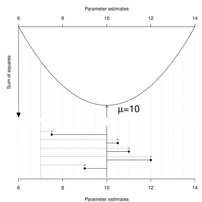
It is clear in the figure above that the sum of the (squared) length of the grey lines that join the observed data to the candidate parameter value of 7 is greater than the sum of the (squared) length of the black lines that join the observed data to the candidate parameter value of 10.

As the differences between observed and predicted are squared (otherwise they would sum to 0), it is assumed that these differences (residuals) are symmetrically distributed around 0. For this reason, they are almost exclusively aligned to the Normal (Gaussian) distribution (as nearly every other useful sampling distribution has the potential to be asymmetric and/or invalid for negative values).

Least squares estimation has no inherent basis for testing hypotheses or constructing confidence. Instead, inference is achieved via manipulating the properties of the residual variance.

Maximum likelihood

The maximum likelihood (ML) approach estimates one or more population parameters such that the (log) likelihood of obtaining the observed sample values from such populations with the nominated probability distribution is maximized. That is, the maximum likelihood parameter estimates are the parameter values that make the observed data most likely.

Likelihood of observed data, given a specific set of distribution parameters (for example the mean $\mu$ and standard deviation $\sigma^2$ of a normal distribution) is the product of the individual densities of each observation for those parameters (and distribution).

$$\mathscr{L}(D|P) = \Pi~f(D_i; P_A, P_B)$$ $$\mathscr{L}(x_1, x_2, ..., X_i|\mu, \sigma^2) = \Pi~f(x_i;\mu,\sigma^2)$$

Computationally, this involves accumulating the probabilities of obtaining each observation for a range of possible population parameter estimates, and using integration to determine the parameter value(s) that maximize the likelihood. A simplified example of this process is represented in the following figure.

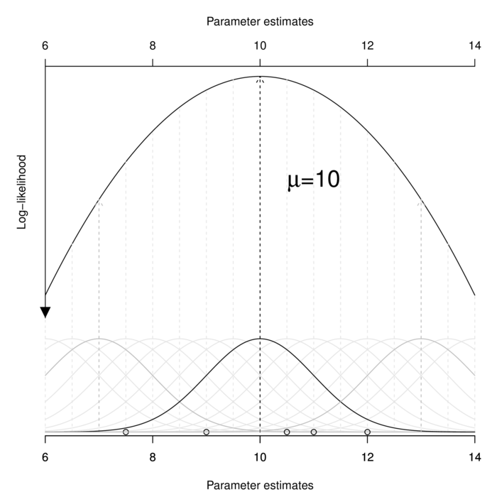
Likelihood can accommodate any exponential probability distribution (such as Normal, binomial, Poisson, gamma or negative binomial). When the nominated probability distribution is Normal (as in the above figure), ML estimators for linear model parameters have exact computational solutions and are identical to LS solutions.

Given enough time, it is possible to determine the exact combination of parameter values (for the nominated distribution) from amongst all possible combinations that maximizes the log-likelihood of observing the collected data by pure brute force (i.e. calculating the log-likelihood from all parameter combinations). For simple models (with few parameters), maximum likelihood estimates can also be obtained algebraically by integrating to the first partial derivative (the local minimum of which is zero). Unfortunately, as models become increasingly more complex (with more parameters), so too does the complexity of the integration. Once the parameter space has more than two parameters, this algebraic solution becomes non-viable and complex optimization routines (such as Newton-Raphson optimization) are necessary. The Newton-Raphson method is an optimization routine that iteratively approaches the root (zero value) of a function by taking the intercept of the tangent of first derivatives of successive root estimates.

Unlike least squares, the maximum likelihood estimation framework also provides standard errors and confidence intervals for estimations (since the negative log-likelihood follows a $\chi^2$) and therefore can provide a basis for statistical inference (for those seeking to apply frequentist interpretation).

A drawback of this procedure is that it is known to be unstable near horizontal asymptotic. Indeed this is one of the main reasons why log-likelihood is preferred over likelihood (log-likelihood functions are steeper and have narrower curvatures and thus have more prominent maxims). It is also known to yield biased parameter estimates (the severity of which is inversely related to sample size in a manner analogous to the degree of bias in estimates of standard deviation). Another major draw back of this method is that it typically requires strong assumptions about the underlying distributions of the parameters.

Bayesian

The Bayesian approach yields (posterior probability) distributions for each of the model parameters. Therefore, a point estimate of each parameter is just the mean (or median or mode) of its posterior distribution.

Recall from Tutorial 4.2 that via the use of very simple and well established laws of conditional probability we can derive Bayes' rule: $$P(H|D) = \frac{P(D|H)imes P(H)}{P(D)}$$ which establishes the relationship between the probability of the parameters given the data and the likelihood of the data given the parameters. In the above rule, $P(H|D)$ (or $P(y|p)$ - probability of data given a parameter), the likelihood of the data, is some density function that describes the likelihood of the observed data for a range of possible parameter combinations and $P(H)$ ($P(p)$) is the prior probability (or expected characteristics) of the parameters.

In essence, the posterior probability distribution is a weighted average of the information contained in the current data (the likelihood) and the prior expectations based on previous studies or intuition. \begin{align*} {posterior~probability} &\sim {likelihood} imes {prior~probability}\\ p(H|D) &\sim \mathscr{L}(D|H)imes P(H) \end{align*}

To qualify as a probability distribution from which certain properties (such as probabilities and confidence intervals) can be gleaned, a distribution (continuous density function) must integrate to one. That is, the total area (or volume) under the function must equal 1. Hence, in order to convert the product of the likelihood and the prior probability into a true probability distribution it is necessary to normalize this product to the appropriate sample space.

From Bayes' rule, this is achieved by division with $P(D)$, the normalizing constant or "marginal likelihood". $P(D)$ is the probability of our data considering the model and is determined by summing across all possible parameter values weighted by the strength of belief of those parameters. $$P(H|D) = \frac{\mathscr{L}(D|H)imes P(H)}{P(H)dH}$$

When there are only a small number of possible parameter (hypothesis values), the calculations are relatively straight forward. For example, if the parameter can only be one of two states ('Male' 'Female'), then the equation becomes: $$P(F|D) = \frac{P(F|H)imes P(F)}{P(F|H)imes P(F) + P(M|H)imes P(M)}$$ where $F$ and $M$ represent parameter values of 'Female' and 'Male' respectively.
However, when $H$ is continuous and the number of possible parameter values (hypotheses) is very large or infinite, it is necessary to integrate over the entire parameter space.

Both frequentist and Bayesian approaches can both start with start with maximum likelihood. However, whilst maximum likelihood parameter estimates are the result of maximizing across all possible parameter values, Bayesian estimates are the result of integrating across all possible parameter values. $$P(H|D) = \frac{\mathscr{L}(D|H)imes P(H)}{\int P(D|H)P(H)dH}$$ Unfortunately, integration of irregular high-dimensional functions (the more parameters, the more dimensions) is usually intractable.

Indeed, the lack of a simple mathematical solution was one of the main reasons that Bayesian statistics initially failed to gain traction.

One way to keep the math simple is to use likelihood functions with "conjugate" prior functions to ensure that the prior function is of the same form as the prior function. It is also possible to substitute the functions with approximations that simplify the algebra.

Markov Chain Monte Carlo sampling

Markov Chain Monte Carlo (MCMC) algorithms provide a powerful, yet relatively simple means of generating samples from high-dimensional distributions. Whilst there are numerous specific MCMC algorithms, they all essentially combine a randomization routine (Monte Carlo component) with a routine that determines whether or not to accept or reject randomizations (Markov Chain component) in a way that ensures that the samples are drawn from multidimensional space proportional to their likelihoods such that the distribution of these samples (posterior probability distribution) reflects their likelihood in high-dimensional space. Given a sufficiently large number of simulations, the resulting samples should exactly describe the target probability distribution and thereby allow the full range of parameter characteristics to be derived.

To illustrate the mechanics of MCMC sampling, I will contrive a very simple scenario in which we have two parameters ($\alpha$ and $\beta$). I will assume infinitely vague priors on both parameters and thus the density function from which to draw samples will simply be the likelihood density function for these parameters. For simplicity sake, this likelihood function will be a multivariate normal distribution for the two parameters with values of $\alpha=0$ ($var=1$) and $\beta=5$ ($var=2$). The following two graphics provide two alternative views (perspective view and contour view) of this likelihood density function.

The specific MCMC algorithm that I will describe is the Metropolis-Hastings algorithm and I will do so as much as possible via visual aids. Initially a location (coordinates) in multi-dimensional space (in this case 2-D) corresponding to a particular set of parameter values is chosen as the starting location. We will start with the coordinates (α=0.5, β=-0.5), yet make the point that if we collect enough samples, the importance of the initial starting configuration will diminish.

The values of the parameters sampled from this joint distribution are then stored.

Now lets move to another random sampling location. To do so, we will move a random multivariate distance and direction from the current location based on the coordinates of a single random location drawn from a multivariate normal distribution centered around zero. The ratio of probabilities (heights on the perspective diagram) corresponding to the new and previous locations is then calculated and this ratio effectively becomes the probability of accepting the new location. For example, the probability associated with the initial location was approximately 0.037 and the probability associated with the new location is 0.019. The probability of moving is therefore 0.019/0.037=0.513. There is just over 50% chance of moving. A random number between 0 and 1 is then drawn from a uniform distribution. If this number is greater than the ratio described above, the new location is rejected and the previous location is resampled. However, if the number is less than the ratio, then the new location is accepted and parameter values are stored from this new location.

The sampling chain continues until a predefined number of iterations have occurred.

With 1000 samples collected

The collected samples, in this case 1000 samples for $\alpha$ and 1000 for $\beta$, can then be used to calculate a range of characteristics.

> colnames(params)<-c("a","b")
> apply(params,2,mean)

          a           b 
-0.03090054  5.22433258

> apply(params,2,sd)

        a         b 
0.8792583 1.4364185

Recall that the true parameter means and standard deviations were ($\alpha=0, var=1 \Rightarrow sd=1; \beta=5, var=2 \Rightarrow sd=1.414$). Whilst the means and standard deviations from the simulated samples are similar to these values, they are in no way identical. There are numerous potential reasons for this. We will now explore these. It is worth noting at this point that we are in the unique position of being able to identify that the parameter estimates do not yet match closely the true parameter values. Normally this would not be case. However, there are various diagnostics that we can employ to help us evaluate whether the chain has yielded a stationary posterior distribution or not.

Perhaps the posterior distribution (represented by the red dots) had not yet stabilized. That is, perhaps the shape of the posterior distribution was still changing slightly with each additional sample collected. The chain had not yet completely sampled the entire surface in approximate proportion to the densities. If so, then collecting substantially more samples could address this. Lets try 10,000.
```
          a           b 
-0.02836663  4.99912614 
```
```
       a        b 
1.010878 1.422975 
```
The resulting estimates are now very accurate. Given sufficient independent MCMC samples, exact solutions can be obtained (c.f. frequentist approximates that become increasingly more dubious with increasing model complexity and diminishing levels of replication).

The "sharper" the features (and more isolated islands) in the multidimensional profile, the more samples will be required in order to ensure that the Markov chain traverses (mixes across) all of the features. One of the best ways of evaluating whether or not sufficient samples have been collected is with a trace plot. Trace plots essentially display the iterative history of MCMC sequences. Ideally, the trace plot should show no trends, just consistent random noise around a stable baseline. Following are three trace plots that depict an adequate number samples, inadequate number of samples and insufficient mixing across all features.
The drawback of a Markov Chain is that the samples are not independent of one another. In a sense, its strength (the properties that allow it to simulate in proportion to the density) can also be a weakness in that consecutive samples are likely to be very similar (non-independent) to one another. Summary statistics based on non-independent samples tend to be biased and can be unrepresentative.

It turns out that there is a very simple remedy for this however. Rather than store every single sample, we can thin the sample set by skipping over (not storing) some of the samples. For example, we could nominate to store every second, or fifth or tenth etc sample. The resulting samples will thence be more independent of one another. Note however, that the sample will be smaller by a factor of the thinning value and thus it may be necessary to perform more iterations.

To illustrate autocorrelation and thinning, we will run the MCMC simulations twice, the first time with no thinning and a second time with a thinning factor of 10. Non-thinned (stored) samples are depicted as circles with black borders. Associated with each chain of simulations, is an autocorrelation function (ACF) plot which represents the degree of correlation between all pairs of samples separated by progressively larger lags (number of samples).
Thinning factor = 1

Thinning factor = 10

For the un-thinned samples, the autocorrelation at lag 1 (adjoining pairs of samples) is over 0.8 (80%) indicating a very high degree of non-independence. Ideally, we would like to aim for a lag 1 autocorrelation value no greater than 0.1. According to the ACF plot associated with the un-thinned simulation chain, to achieve a lag 1 autocorrelation value of no greater than 0.1 would require a sample separation (thinning) of greater than 10. Indeed, the second simulation chain had a thinning factor of 10 (only retained every 10th sample) and still has a lag 1 autocorrelation value greater than 0.1 (although this is may now be because it is based on a much smaller sample size). To be sure, we could re-simulate the chain again with a 15-fold thinning but with 10 times more iterations (a total of 10,000).
Although the importance of the starting configuration (initial coordinates) should eventually diminish as the stochastic walk traverses more and more of the profile, for shorter chains, the initial the initial path traversed is likely to exert a pull on the sample values. Of course, substantially increasing the number of iterations of the chain will substantially increase the time it takes to run the chain.

Hence, it is common to define a burnin interval at the start of the chain. This defines the number of initial iterations that are ignored (samples not retained). Generally, ignoring the first 10% of iterations should be sufficient. In the current artificial example, this is unlikely to be an issue as the density distribution has very blunt, connected features.

Eventually (given enough iterations), the MCMC chain should sample the entire density profile and the resulting posterior distribution should converge (produce relatively invariant outcomes) on a stationary distribution (the target distribution).

Unlike models fitted via maximum likelihood (which stop iterating when the improvement in log-likelihood does not exceed a pre-defined value - at which point they have usually converged), MCMC chains do not have a stopping criterion. Rather, the analyst must indicate the number of iterations (simulations) to perform. The number of iterations is always a compromise between convergence and time. The more iterations, the better the mixing and coverage, the greater the likelihood of convergence, yet the greater the time it takes to complete the analysis.

Trace plots - as described above, trace plots for each parameter offer visual indicators of issues with the mixing and coverage of the samples collected by the chain as well as the presence of a starting configuration impact. In addition to the lack of drift, the residuals (sometimes called units) should be centered around 0. Positive displacement of the residuals can be an indication of zero-inflation (response having more zeros that the modelling distribution should expect).
Plots of the posterior distribution (density or histograms) of each parameter. The basic shape of these plots should follow the approximate expected joint probability distribution (between family modeled in determining likelihood and prior). Conjugate priors are typically used to simplify the expected posterior distribution.

In our contrived example, this should be a normal distribution. Hence, obviously non-normal (particularly bi-modal) distributions would suggest that the chain has not yet fully mixed and converged on a stationary distribution. Specifically, it would imply that the sampling chain had focused heavily on one region of the parameter space before moving and focusing on another region. In the case of expected non-normal distributions, the density plots can also serve to remind us that certain measures of location and spread (such as mean and variance) might be inadequate characterizations of the population parameters.
Autocorrelation - correlation between successive samples (as a result of way the Markov Chain spreads) are useful for determining the appropriate amount of thinning required to generate a well mixed series of samples. Autocorrelation can be explored visually (in a plot such as that illustrated earlier) or numerically by simply exploring the autocorrelation values at a range of lags.
The Geweke diagnostic (and Geweke-Brooks plot) compares the means (by a standard Z-score) of two non-overlapping sections of the chain (by default the first 10% and the last 50%) to explore the likelihood that the samples from the two sections come from the same stationary distribution. In the plot, successively larger numbers of iterations are dropped from the start of the samples (up to half of the chain) and the resulting Z-scores are plotted against the first iteration in the starting segment.

Substantial deviations of the Z-score from zero (those outside the horizontal critical confidence limits) imply poor mixing and a lack of convergence. The Geweke-Brooks plot is also particularly useful at diagnosing a lack of mixing due o the initial configuration and how long the burnin phase should be.
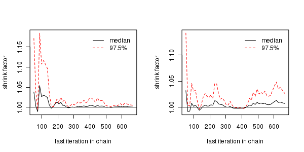
The Gelman and Rubin diagnostic essentially calculates the ratio of the total variation within and between multiple chains to the within chain variability (this ratio is called the Potential Scale Reduction Factor). As the chain progresses (and samples move towards convergence) the variability between chains should diminish such that the scale reduction factor essentially measures the ratio of the within chain variability to itself. At this point (when the potential scale reduction factor is 1), it is likely that any one chain should have converged. When the potential scale reduction factor is greater than 1.1 (or more conservatively 1.2), we should run the chain(s) for longer to improve convergence.

Clearly, in order to calculate the Gelman and Rubin diagnostic and plot, it is necessary to run multiple chains. When doing so, it is advisable that different starting configurations be used for each chain.
A Raftery and Lewis diagnostic estimates the number of iterations and the burnin length required to have a given probability (95%) of posterior quantile (0.025) accuracy (0.005). In the following, I will show the Raftery and Lewis diagnostic from a sample length of 1000 (which it considers below the minimum requirements for the quantile, probability and accuracy you have nominated) and this will be followed by diagnostics from a longer chain (40,000 iterations with a thinning factor of 10). In the latter case, for each parameter it lists the burnin length ($M$), number of MCMC iterations ($N$), minimum number of (uncorrelated) samples to construct this plot and $I$ (the proportional increase in necessary iterations due to autocorrelation). Values of $I$ greater than 5 indicate substantial autocorrelation.
```
Quantile (q) = 0.025
Accuracy (r) = +/- 0.005
Probability (s) = 0.95 

You need a sample size of at least 3746 with these values of q, r and s
```
```
Quantile (q) = 0.025
Accuracy (r) = +/- 0.005
Probability (s) = 0.95 
                                       
 Burn-in  Total Lower bound  Dependence
 (M)      (N)   (Nmin)       factor (I)
 4        4782  3746         1.28      
 5        5894  3746         1.57      
```
The Heidelberg and Welch diagnostic tests a null hypothesis that the Markov chain is from a stationary distribution. The test evaluates the accuracy of the estimated means after incrementally discarding more and more (10%, 20%, 30% up to 50%) of the chain. The point at which the null hypothesis is accepted marks the number of iterations required to keep. If the null hypothesis is not accepted by the time 50% of the chain has been discarded, it suggests that more MCMC iterations are required to reach a stationary distribution and to estimate the mean with sufficient accuracy. For the portion of the chain that passed (null hypothesis accepted), the sample mean and 95% confidence interval are calculated.

If the ratio of the mean to 95% interval is greater than 0.1, then the mean is considered accurate otherwise a longer overall chain length is recommended. Note, this diagnostic is misleading for residuals or any other parameters whose means are close to zero. Whilst this diagnostic can help trim chains to gain speed, in practice it is more useful for just verifying that the collected chain is long enough.
```
                                
  Stationarity start     p-value
  test         iteration        
a passed       1         0.326  
b passed       1         0.713  
                            
  Halfwidth Mean   Halfwidth
  test                      
a failed    0.0262 0.0902   
b passed    5.0083 0.1438   
```
```
                                   
     Stationarity start     p-value
     test         iteration        
[,1] passed       1         0.245  
[,2] passed       1         0.912  
                               
     Halfwidth Mean   Halfwidth
     test                      
[,1] failed    -0.017 0.0395   
[,2] passed     5.003 0.0683   
```

Although MCMC algorithms have their roots in the Bayesian paradigm, they are not exclusively bound to Bayesian analyses. Philosophical arguments aside, MCMC sampling algorithms provide very powerful ways to tackling otherwise intractable statistical models. Indeed, it is becoming increasingly more common for MCMC sampling to employ vague (non-informative) priors to fit models that are otherwise not analytically compliant or convergent.

Priors

Bayesian analyses incorporate prior expectations about the parameters being estimated (fixed effects, random effects and residuals). As with the likelihoods and posteriors, the priors are distributions (rather than single values) thereby reflecting the typical prior expectations as the variability (spread).

Whilst proponents consider the ability to evaluate information within a broader and more substantive context is one of the great strengths of the Bayesian framework, opponents claim that the use or reliance of prior information has the potential to bias the outcomes. To an extent, both camps have valid points (which is perhaps why the philosophical debates continue). However, there is a practical compromise.

It is possible, and indeed advisable to employ a range of priors including non-informative (or null, vague, weakly informative) priors. Strickly, non-informative priors (such as a uniform distribution which is purely flat over its entire range) have no impact on the outcomes as they simply multiply the likelihood by a constant. Hence, non-informative flat priors result in parameter estimates that are almost identical to those of equivalent traditional analyses.

Weakly informative priors (which are typically more preferable) impose a broad structure (e.g. the prior of a parameter is normally distributed with a certain mean and typically very large standard deviation). Whilst in the absence of any other prior knowledge, it is common to use a normal distribution with a mean of zero and very large standard deviation. Note however, that such a prior distribution will have the effect of 'shrinking' estimates towards zero. Such priors are very useful when no other priors are sensible and justifiable. By applying a range of priors, it is possible to evaluate the impact of different priors and this in itself can be a valuable form of analysis.

Even when no prior information is available, priors must still be defined to make use of MCMC sampling techniques. In such cases, non-informative priors are typically defined.

The other retort to the subjectivity accusation is that science is an inherently subjective activity in the first place. To deny there is no subjectivity in other aspects of sampling design and data collection is purely fanciful. At least in the case of selecting priors, we can (by using a range of priors) at least evaluate this source of bias.

Conjugate priors

Although priors can be specified from any distribution, historically the choice of distribution was such that the posterior distribution could be calculated via relatively simple hand calculations. Recall that the posterior distribution is equal to the product of the likelihood function ($P(D|H)$) and the prior ($P(H)$) normalized (divided by) the probability of the data ($P(D)$) and that $P(D)$ is determined by integrating across all possible parameter (hypothesis) values. $$P(H|D) = \frac{P(D|H)imes P(H)}{\int P(D|H)P(H)dH}$$ Calculating the integral ($\int P(D|H)P(H)dH$) is generally more manageable when the posterior distribution ($P(H|D$) is the same distribution family (same distribution type, yet possibly different values of the parameters) as the prior distribution ($P(H)$). The posterior and prior distributions are thence called conjugate distributions and the prior is considered the conjugate prior to the model likelihood.

A table of the most common conjugate priors follows:

Observations	Likelihood distribution	Parameter	Conjugate prior	Prior hyperparameters
Normal (measurements)	Normal (Gaussian)	$\mu$	normal	$\mu,au$
Normal (measurements)		$au$	gamma	$r,\mu$
Skewed normal (measurements)	Log-normal	$\mu$	normal	$\mu,au$
Skewed normal (measurements)		$au$	gamma	$r,\mu$
Binary (presence/absence, dead/alive)	Binomial or negative binomial	$logit(p)$	beta	$a, b$
		$probit(p)$	gamma	$a, b$
		$cloglog(p)$	gamma	$a, b$
Poisson (counts)	Poisson	$log(\lambda)$	gamma	$r, \mu$
	Negative binomial	$logit(p)$	beta	$a, b$
Percentages	Beta	$a$	beta	$a, b$
		$b$	beta	$a, b$

Note, vague gamma priors has a is relatively flat density over most of its range, yet tend to have a sharp spike at the origin. This can cause problems, particularly in multilevel models. Consequently, uniform priors are recommended as an alternative to gamma priors.

The need for the conjugacy as a mathematical convenience is now unnecessary thanks to MCMC sampling techniques. Nevertheless, conjugacy does make it easier to anticipate the distribution of the posterior(s) and thus help identify and diagnose issues of mixing and convergence (via a lack of conformity to the anticipated distribution).

Priors on variance

Numerous non-informative priors for variance have been suggested including:

flat uniform prior distribution $U(0, A)$, where $A \rightarrow\infty$
non-informative inverse-gamma $Gamma(\epsilon, \epsilon)$, where $\epsilon$ is set to a low value such as 0.001, 1.0E-06 etc)
half-cauchy distribution $HC(\alpha)$ where the scale parameter, $\alpha$ is typically 5 or 25.

Gelman (2006) warns that the use of the inverse-gamma family of non-informative priors are very sensitive to $\epsilon$ particularly when variance is close to zero and this may lead to unintentionally informative priors. When the number of groups (treatments or varying/random effects) is large (more than 5), Gelman (2006) advocated the use of either uniform or half-cauchy priors. Yet when the number of groups is low, Gelman (2006) indicates that uniform priors have a tendency to result in inflated variance estimates. Consequently, half-cauchy priors are generally recommended for variances.

References

Gelman, A. (2006). “Prior distributions for variance parameters in hierarchical models”. In: Bayesian Analysis, pp. 515-533.