Tutorial 8.4a - Dealing with spatial autocorrelation

02 Mar 2018

Important opening note

Dealing with spatial autocorrelation and analysing spatial trends are not the same thing. The former attempts to counter the lack of independence associated with spatial data whereas the later attempts to model the influence of spatial patterns. This tutorial will focus only on spatial autocorrelation, spatial analyses will be the focus of another tutorial.

Spatial autocorrelation

For statistical purposes, time is a one dimensional autocorrelation influence. Differences in time between any sets of time points, is the same no matter which time point is considered first and which is second. By contrast, contagious processes occurring in space operate in two dimensions (influences can radiate out around a point in any direction). So the degree to which sampling units are correlated is influenced by the two dimensional euclidean distance between the two units. Thus, spatial autocorrelation can be thought of as a two dimensional generalization of temporal autocorrelation where the correlation between two locations ($\rho$) is proportional to the euclidean distance between the locations.

One simple correlation structure that works well for spatial autocorrelation defines the covariances as being proportional to the exponential of the product of the distance ($D$) multiplied by the (negative) of the rate of correlation decay ($\delta$). If the rate of decay ($\delta=0.08$), then at a distance of 1 unit, the degree of correlation would be $e^{-0.08}=$0.9231163 and the correlation at a distance of 2 would be $e^{-0.08\times 2}=$0.8521438 and so on in a deminishing manner.

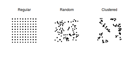
$$ cor(\varepsilon) = \underbrace{ \begin{pmatrix} 1&e^{-\delta}&\cdots&e^{-\delta D}\\ e^{-\delta}&1&\cdots&\vdots\\ \vdots&\cdots&1&\vdots\\ e^{-\delta D}&\cdots&\cdots&1\\ \end{pmatrix}}_\text{Exponential autoregressive correlation structure} $$

An important consideration when it comes to spatial influences is how regular the sampling units are distributed in space. The following figure demonstrates a range of configurations from a regular grid to a random scatter to clumped arrangement.

As is the way of these tutorials, we will now generate some fabricated data in order to explore spatial autocorrelation. We will generate one hundred locations (latitude nd longitude) from within a spatial grid

set.seed(3)  #4,8,12,15,16,33,47,49,50
n <- 100
# simgrid <-
# expand.grid(LAT=runif(10,144,150),LONG=runif(10,-26,-20))
# n <- nrow(simgrid) library(sp)
loc <- data.frame(LAT = runif(n, 144, 150), LONG = runif(n,
    -26, -20))

library(sp)
grid <- expand.grid(LAT = seq(144, 150, l = 100), LONG = seq(-26,
    -20, l = 100))
coordinates(grid) <- ~LAT + LONG
# loc <- spsample(grid, n=n, type='random') loc <-
# data.frame(spsample(grid, n=n, type='regular'))
# names(loc) <- c('LAT','LONG') coordinates(loc) <-
# ~LAT+LONG

# Set up distance matrix
distance <- as.matrix(dist(as.data.frame(loc)))  #* 1/min(distance[lower.tri(distance)])
# Generate random variable
delta <- 0.5
Vmat <- function(n, mu = 0, V = matrix(1)) {
    p <- length(mu)
    if (any(is.na(match(dim(V), p))))
        stop("Dimension problem!")
    D <- chol(V)
    t(matrix(rnorm(n * p), ncol = p) %*% D + rep(mu,
        rep(n, p)))
}
V <- Vmat(1, rep(0, n), exp(-delta * distance))
x <- rnorm(n, 30, 10)
# image(cbind(simgrid, V))
y <- 50 + 1 * x + 60 * V  #+ rnorm(n,0,1)
data.spatialCor <- data.frame(y, x, loc)
write.table(data.spatialCor, file = "../downloads/data/data.spatialCor.csv",
    sep = ",", quote = FALSE, row.names = FALSE)
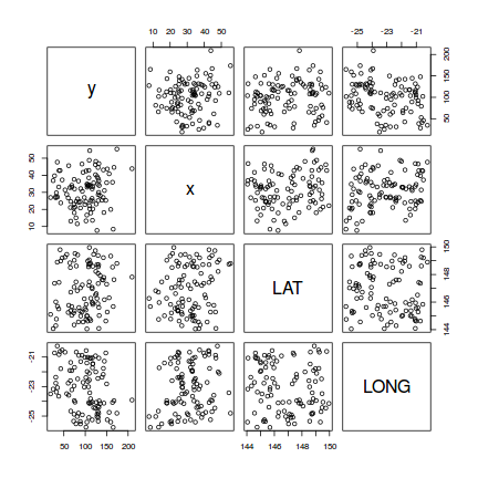
pairs(data.spatialCor)

# coordinates(data.spatialCor) <-~LAT+LONG
# bubble(data.spatialCor,'y')

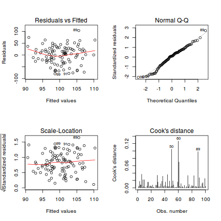
As the primary focus of the analyses is to investigate the relationship between y and x, we will begin by fitting a standard simple linear regression and then explore the model fit diagnostics.

data.spatialCor.lm <- lm(y ~ x, data.spatialCor)
par(mfrow = c(2, 2))
plot(data.spatialCor.lm, which = 1:4)

Conclusions - so far so good.

Detecting spatial autocorrelation

The bubble plot

The observations have been collected across a wide spatial scale. Wide in the sense that the total area is likely to span many underlying environmental gradients that will represent multiple contageous processes - thereby potentially resulting in substantial spatial autocorrelation. Therefore, it is worth investigating whether there is any evidence of spatial autocorrelation in the data.

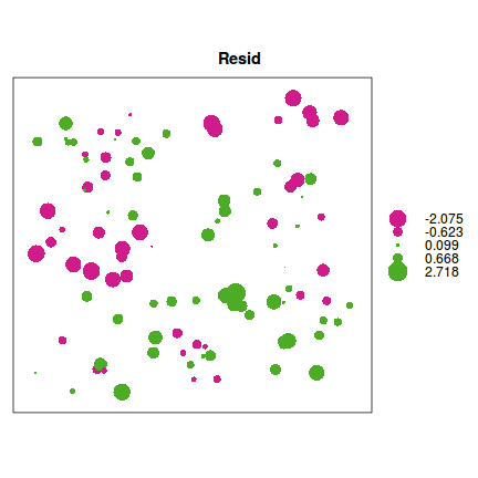
One relatively simple way of detecting spatial autocorrelation is to explore whether there are any spatial patterns in the residuals. To do this, we plot the sampling unit coordinates (latitude and longitude) such that the size, shape and or colors of the points reflect the residuals associated with these observations. Such a plot is referred to as a bubble plot.

The sp package is a large collection of functions and classes specifically for working with spatial data. To leverage these functions, we must first define the spatial nature of the data. That is, we need to declare which variables represent the spatial coordinates. Note, it is also possible to define the coordinate reference (or projection) system, however this is only required if you intend to perform complex spatial operations or conversions to other projection systems.

Bubble plots are generated via the bubble() function (of the sp package). At a minimum, this function requires a spatial data frame (a data frame with defined coordinates) that contains the model residuals.

data.spatialCor$Resid <- rstandard(data.spatialCor.lm)
library(sp)
coordinates(data.spatialCor) <- ~LAT + LONG  #effectively convert the data into a spatial data frame
bubble(data.spatialCor, "Resid")

Conclusions - there is a clear spatial pattern in the residuals. Observations with similar residuals come from sampling units that were closer together in space and thus there is evidence of spatial autocorrelation.

The semi-variogram

A more formal and quantitative alternative to exploring spatial autocorrelation is to calculate semivariance. Semivariance is a measure of the degree of similarity between pairs of points separated by a specific distance. If the data are spatial autocorrelated, then sampling units that are closer together in space might be expected to yield similar responses and thus similar residuals. There are numerous ways to calculate semivariance, yet in all cases, it is essentially the variance of residuals from points separated by a particular distance. Points that are closer together in space are likely to have smaller values of semivariance.

As every set of actual points are likely to represent a unique distance, distances are effectively binned such that all points spanning a band of distances in a particular direction (say north of each point in turn) are aggregated together when calculating the variance in residuals for that distance.

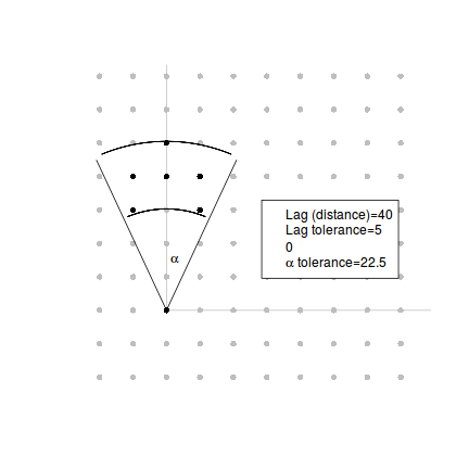
The following figure loosely describes the calculations. For each point (in this instance, a point 3 units left and 3 units north on the grid), all other points within a certain tolerance band from a distance (lag, in this case 40 units) in a particular direction (in this case north, or an angle of 0 degrees) from the reference point are aggregated together. The tolerance band is bound by a shape that is the lag plus and minus the lag tolerance (in this case 5) and the direction angle plus or minus the tolerance in the angle (22.5 degrees in this case).

For situations in which the underlying contagious processes (that cause spatial autocorrelation) radiate out uniformly, the orientation (N, NE, E, SE etc) that we elect to calculate semivariance will be inconsequential (the semivariances are said to be isotropic). However, when the contagious process(es) spread asymmetrically (for example, due to wind direction and speed), the orientation will be important and the semivariances will depend on the direction of measurement (anisotropy).

Semivariance is then plotted against distance as a variogram.

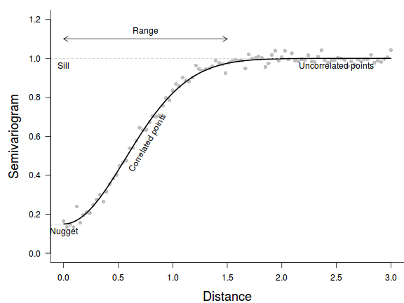
Points separated by small distances are similar and thus have relatively small values of semivariance. In spatially correlated data, semivariance increases with increasing distance up to a point (the sill). The span of distances over which points are correlated is called the range.

Whilst we might expect the value of semivariance at a distance of zero to be zero, in reality we rarely have sampling units that approach such a small distance from one another. The value of semivariance when distance is equal to zero (the nugget is often estimated to be higher than zero. Typically this is the result of unexpected variability in your data that spatial patterns alone cannot account for.

It is also possible for the semivariogram values to peak at a value of close to 1 before declining again. This would imply sampling unit similarity declines with increasing spatial separation up to a certain distance above which sampling units spread further apart begin to become more similar. Such a situation can arise when the underlying environmental gradients governing the radiation of contagious processes cycle across the landscape. For example, imagine sampling throughout a landscape that features numerous different vegetation communities. At some point the local processes driving small scale spatial autocorrelation will be overtaken by the larger scale processes driving broad community changes.

So having explained all that, lets now generate a variogram plot and to formally assess spatial autocorrelation. As with temporal autocorrelation, it is best to switch from using the lm() function to using the Generalized least Squares (GLS: gls()) function from the nlme package.

We should also explore the usual suite of model diagnostics.

data.spatialCor.gls <- gls(y ~ x, data.spatialCor,
    method = "REML")
plot(data.spatialCor.gls)

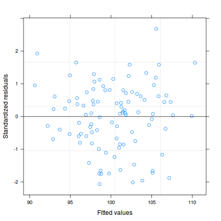
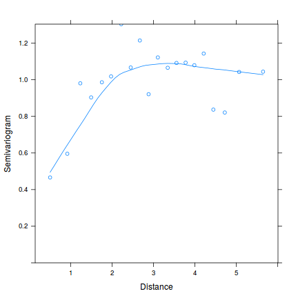
Conclusions - there are no obvious signs of issues with normality or homogeneity of variance so far. However as this section is primarily concerned with spatial autocorrelation, it is this issue that we will now focus on.

There are two similar functions for generating variograms in R. The first we will explore is a function called Variogram() that comes with the nlme package.

plot(nlme:::Variogram(data.spatialCor.gls, form = ~LAT +
    LONG, resType = "normalized"))

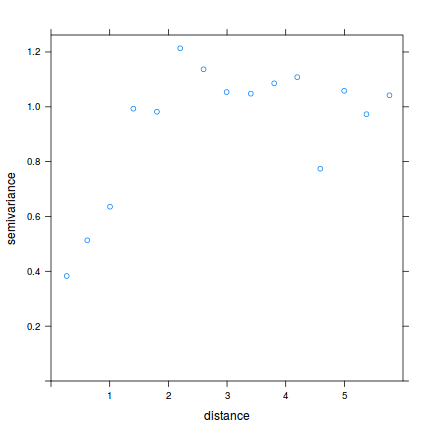
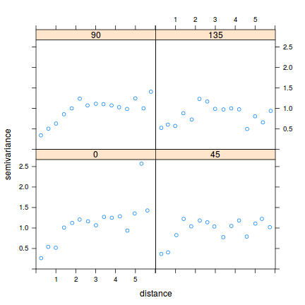
The second, is the more flexible variogram function from the gstat package. Along with the default variagram calculated along a vertical direction (orientation angle of zero), there is the option to indicate additional orientations (via a alpha= parameter). Useful additional orientations would be North-East, East, South-East which respectively translate to alpha values of 45,90,135. Note, a alpha of 180 (South) would be the same as that of North.

By calculating the variogram separately at different orientations, we can get a handle on whether the underlying contagious process(es) (and thus spatial autocorrelation) is likely to be symmetrical (isotrophy) or asymmetrical (anisotropy).

library(gstat)
plot(variogram(residuals(data.spatialCor.gls, "normalized") ~
    1, data = data.spatialCor, cutoff = 6))

plot(variogram(residuals(data.spatialCor.gls, "normalized") ~
    1, data = data.spatialCor, cutoff = 6, alpha = c(0,
    45, 90, 135)))

Conclusions - there is clear evidence of spatial autocorrelation. The semivariogram values increase up to a point (close to a sill of 1) before plateauing). The separate variograms for different orientations are all very similar to one another, suggesting that the spatial autocorrelation is relatively symmetrical.

Moran's I

coords = cbind(data.spatialCor$LONG, data.spatialCor$LAT)
w = fields:::rdist(coords)
library(ape)
Moran.I(x = data.spatialCor$y, w = w)

$observed
[1] -0.04542672

$expected
[1] -0.01010101

$sd
[1] 0.005916655

$p.value
[1] 2.364483e-09

Accommodating spatial autocorrelation in the model

If we were primarily interested in the relationship between y and x and wished to standardize for spatial patterns, then we could attempt to incorporate into the model some additional covariates that we believe drives the underlying spatial patterns. However, meaningful and causal influences are often either very difficult to identify or else extremely difficult to measure - particularly if spatial autocorrelation is not considered until after the data have been collected.

As an alternative we could add the multiplicative effects of latitude and longitude to the model as proxies for the underlying contagion. However, the resulting hypothesis associated with the spatial factors are somewhat meaningless - latitude is highly unlikely to be the direct cause of variation in responses. Furthermore, adding these terms will absorb 3 degrees of freedom from the model.

More importantly, the above solutions do not directly address the issues of dependency structure. It is for this reason, that it is arguably better to address spatial autocorrelation by modelling in some form of spatial dependence correlation structure.

In the introduction to spatial autocorrelation, I illustrated an exponential autoregressive correlation structure. Recall that this is a correlation structure in which the degree of correlation degrades according to the exponential of the product of the distance and the rate of correlation decay ($e^{-\delta D}$).

This is not the only correlation structure useful for accommodating spatial autocorrelation. The causes of spatial autocorrelation are many and varied and thus so too are the theoretical manners in which sampling units could be correlated over space. Additionally, the configuration of sampling units across space (recall the gridded, random and clustered configurations) also impact on the manner in which autocorrelation manifests in data.

The following table and figure illustrate the correlation structures built into the nlme package as well as the general form of variogram they accommodate. Note all of these assume isotrophy.

correlation function	Correlation structure	Description
`corExp(form=~lat+long)`	Exponential	$\Phi = 1-e^{-D/\rho}$
`corGaus(form=~lat+long)`	Gaussian	$\Phi = 1-e^{-(D/\rho)^2}$
`corLin(form=~lat+long)`	Linear	$\Phi = 1-(1-D/\rho)I(d<\rho)$
`corRatio(form=~lat+long)`	Rational quadratic	$\Phi = (d/\rho)^2/(1+(d/\rho)2)$
`corSpher(form=~lat+long)`	Spherical	$\Phi = 1-(1-1.5(d/\rho) + 0.5(d/\rho)^3)I(d<\rho)$

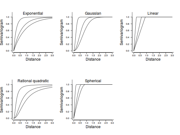
Based on the variogram we generated from the first fitted model we tried, it would seem like the exponential or rational quadratic are good candidate correlation structures for our data. That said, most argue that it is appropriate to fit all alternative models and then select the model with the lowest AIC.

data.spatialCor.glsExp <- gls(y ~ x, data = data.spatialCor,
    correlation = corExp(form = ~LAT + LONG, nugget = TRUE),
    method = "REML")
data.spatialCor.glsGaus <- gls(y ~ x, data = data.spatialCor,
    correlation = corGaus(form = ~LAT + LONG, nugget = TRUE),
    method = "REML")
data.spatialCor.glsLin <- gls(y ~ x, data = data.spatialCor,
    correlation = corLin(form = ~LAT + LONG, nugget = TRUE),
    method = "REML")
data.spatialCor.glsRatio <- gls(y ~ x, data = data.spatialCor,
    correlation = corRatio(form = ~LAT + LONG, nugget = TRUE),
    method = "REML")
data.spatialCor.glsSpher <- gls(y ~ x, data = data.spatialCor,
    correlation = corSpher(form = ~LAT + LONG, nugget = TRUE),
    method = "REML")

AIC(data.spatialCor.gls, data.spatialCor.glsExp, data.spatialCor.glsGaus,
    data.spatialCor.glsLin, data.spatialCor.glsRatio,
    data.spatialCor.glsSpher)

                         df       AIC
data.spatialCor.gls       3 1013.9439
data.spatialCor.glsExp    5  974.3235
data.spatialCor.glsGaus   5  976.4422
data.spatialCor.glsLin    5  975.5760
data.spatialCor.glsRatio  5  974.7862
data.spatialCor.glsSpher  5  975.5244

AIC(data.spatialCor.gls, data.spatialCor.glsExp, data.spatialCor.glsGaus,
    data.spatialCor.glsRatio, data.spatialCor.glsSpher)

                         df       AIC
data.spatialCor.gls       3 1013.9439
data.spatialCor.glsExp    5  974.3235
data.spatialCor.glsGaus   5  976.4422
data.spatialCor.glsRatio  5  974.7862
data.spatialCor.glsSpher  5  975.5244

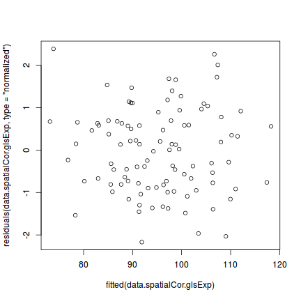
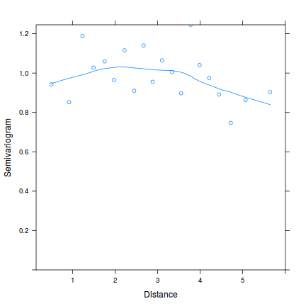
Conclusions - on the basis of AIC, the exponential correlation structure would be considered the 'best'. Note, the model that did not incorporate any correlation structure is substantially worse than any of the correlation structures.

Prior to exploring the parameter estimates, it is (as always) a good idea to examine the model diagnostics.

plot(residuals(data.spatialCor.glsExp, type = "normalized") ~
    fitted(data.spatialCor.glsExp))

plot(nlme:::Variogram(data.spatialCor.glsExp, form = ~LAT +
    LONG, resType = "normalized"))

Conclusions - all good!

Finally, lets compare the output of the original model (that did not incorporate any correlation structure) with the model incorporating an exponential correlation structure.

summary(data.spatialCor.gls)

Generalized least squares fit by REML
  Model: y ~ x 
  Data: data.spatialCor 
       AIC      BIC   logLik
  1013.944 1021.699 -503.972

Coefficients:
               Value Std.Error  t-value p-value
(Intercept) 87.47075 12.481828 7.007847  0.0000
x            0.41275  0.381414 1.082146  0.2818

 Correlation: 
  (Intr)
x -0.951

Standardized residuals:
        Min          Q1         Med          Q3 
-2.06257434 -0.61771240  0.09787811  0.65807028 
        Max 
 2.68271927 

Residual standard error: 38.59125 
Degrees of freedom: 100 total; 98 residual

anova(data.spatialCor.gls)

Denom. DF: 98 
            numDF  F-value p-value
(Intercept)     1 675.7153  <.0001
x               1   1.1710  0.2818

summary(data.spatialCor.glsExp)

Generalized least squares fit by REML
  Model: y ~ x 
  Data: data.spatialCor 
       AIC      BIC    logLik
  974.3235 987.2484 -482.1618

Correlation Structure: Exponential spatial correlation
 Formula: ~LAT + LONG 
 Parameter estimate(s):
    range    nugget 
1.6956723 0.1280655 

Coefficients:
               Value Std.Error  t-value p-value
(Intercept) 65.90018 21.824752 3.019516  0.0032
x            0.94572  0.286245 3.303886  0.0013

 Correlation: 
  (Intr)
x -0.418

Standardized residuals:
       Min         Q1        Med         Q3 
-1.6019483 -0.3507695  0.1608776  0.6451751 
       Max 
 2.1331505 

Residual standard error: 47.68716 
Degrees of freedom: 100 total; 98 residual

anova(data.spatialCor.glsExp)

Denom. DF: 98 
            numDF  F-value p-value
(Intercept)     1 23.45923  <.0001
x               1 10.91566  0.0013

Conclusions - from the model that did not account for spatial autocorrelation, we would have concluded that there was no inferential evidence of a relationship between y and x, however when accounting for spatial autocorrelation, we would conclude that there is a positive correlation between y and x.