Workshop 9 - Generalized linear models

14 September 2011

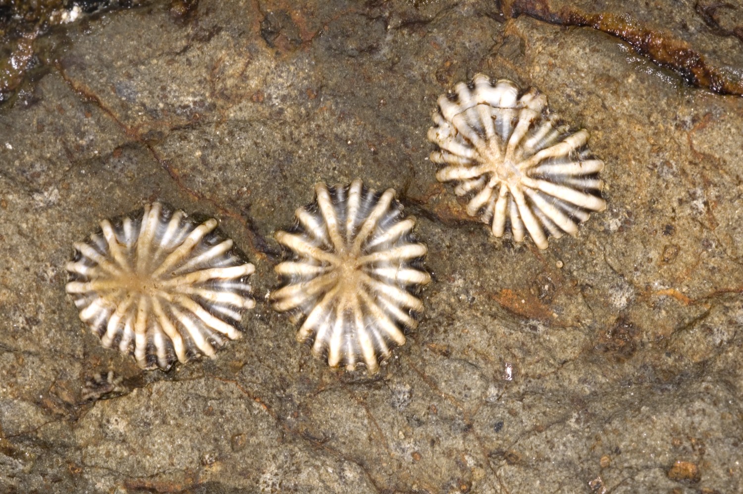
A marine ecologist was interested in examining the effects of wave exposure on the abundance of the striped limpet Siphonaria diemenensis on rocky intertidal shores. To do so, a single quadrat was placed on 10 exposed (to large waves) shores and 10 sheltered shores. From each quadrat, the number of Siphonaria diemenensis were counted.

Download Limpets data set

Format of limpets.csv data files
Count Shore 1 sheltered 3 sheltered 2 sheltered 1 sheltered 4 sheltered ... ... Shore Categorical description of the shore type (sheltered or exposed) - Predictor variable Count Number of limpets per quadrat - Response variable

Open the limpet data set.

> limpets <- read.table("../downloads/data/limpets.csv", header = T,
+     sep = ",", strip.white = T)
> limpets
   Count     Shore
1      2 sheltered
2      2 sheltered
3      0 sheltered
4      6 sheltered
5      0 sheltered
6      3 sheltered
7      3 sheltered
8      0 sheltered
9      1 sheltered
10     2 sheltered
11     5   exposed
12     3   exposed
13     6   exposed
14     3   exposed
15     4   exposed
16     7   exposed
17    10   exposed
18     3   exposed
19     5   exposed
20     2   exposed

The design is clearly a t-test as we are interested in comparing two population means (mean number of striped limpets on exposed and sheltered shores). Recall that a parametric t-test assumes that the residuals (and populations from which the samples are drawn) are normally distributed and equally varied.

> boxplot(Count ~ Shore, data = limpets)

1. The assumption of normality has been violated?
2. The assumption of homogeneity of variance has been violated?

At this point we could transform the data in an attempt to satisfy normality and homogeneity of variance. However, there are likely to be zero values in the data and moreover, it has been demonstrated that transforming count data is not as effective as modelling count data with a Poisson distribution.

> limpets.glm <- glm(Count ~ Shore, family = poisson, data = limpets)

1. Check the model for lack of fit via:
   • Pearson Χ²
     Show code

     > limpets.resid <- sum(resid(limpets.glm, type = "pearson")^2)
     > 1 - pchisq(limpets.resid, limpets.glm$df.resid)
     [1] 0.07875
     > #No evidence of a lack of fit
     

   • Deviance (G²)
     Show code

     > 1 - pchisq(limpets.glm$deviance, limpets.glm$df.resid)
     [1] 0.05287
     > #No evidence of a lack of fit
     

   • Standardized residuals (plot)
     Show code

     > plot(limpets.glm)
     
     
     
     
     

2. Estimate the dispersion parameter to evaluate over dispersion in the fitted model
   • Via Pearson residuals
     Show code

     > limpets.resid/limpets.glm$df.resid
     [1] 1.501
     > #No evidence of over dispersion
     

   • Via deviance
     Show code

     > limpets.glm$deviance/limpets.glm$df.resid
     [1] 1.591
     > #No evidence of over dispersion
     

3. Compare the expected number of zeros to the actual number of zeros to determine whether the model might be zero inflated.
   • Calculate the proportion of zeros in the data
     Show code

     > limpets.tab <- table(limpets$Count == 0)
     > limpets.tab/sum(limpets.tab)
     
     FALSE  TRUE 
      0.85  0.15 
     

   • Now work out the proportion of zeros we would expect from a Poisson distribution with a lambda equal to the mean count of limpets in this study.
     Show code

     > limpets.mu <- mean(limpets$Count)
     > cnts <- rpois(1000, limpets.mu)
     > limpets.tab <- table(cnts == 0)
     > limpets.tab/sum(limpets.tab)
     
     FALSE  TRUE 
     0.955 0.045 
     

     There are not substantially higher proportion of zeros than would be expected. Clearly there are not more zeros than expected so the data are not zero inflated.

1. Wald z-tests (these are equivalent to t-tests)
Show code

> summary(limpets.glm)

Call:
glm(formula = Count ~ Shore, family = poisson, data = limpets)

Deviance Residuals: 
    Min       1Q   Median       3Q      Max  
-1.9494  -0.8832   0.0719   0.5791   2.3662  

Coefficients:
               Estimate Std. Error z value Pr(>|z|)    
(Intercept)       1.569      0.144   10.87  < 2e-16 ***
Shoresheltered   -0.927      0.271   -3.42  0.00063 ***
---
Signif. codes:  0 '***' 0.001 '**' 0.01 '*' 0.05 '.' 0.1 ' ' 1 

(Dispersion parameter for poisson family taken to be 1)

    Null deviance: 41.624  on 19  degrees of freedom
Residual deviance: 28.647  on 18  degrees of freedom
AIC: 85.57

Number of Fisher Scoring iterations: 5

2. Wald Chisq-test. Note that Chisq = z²
Show code

> library(car)
> Anova(limpets.glm, test.statistic = "Wald")
Analysis of Deviance Table (Type II tests)

Response: Count
          Df Chisq Pr(>Chisq)    
Shore      1  11.7    0.00063 ***
Residuals 18                     
---
Signif. codes:  0 '***' 0.001 '**' 0.01 '*' 0.05 '.' 0.1 ' ' 1 

3. Likelihood ratio test (LRT), analysis of deviance Chisq-tests (these are equivalent to ANOVA)
Show code

> limpets.glmN <- glm(Count ~ 1, family = poisson, data = limpets)
> anova(limpets.glmN, limpets.glm, test = "Chisq")
Analysis of Deviance Table

Model 1: Count ~ 1
Model 2: Count ~ Shore
  Resid. Df Resid. Dev Df Deviance Pr(>Chi)    
1        19       41.6                         
2        18       28.6  1       13  0.00032 ***
---
Signif. codes:  0 '***' 0.001 '**' 0.01 '*' 0.05 '.' 0.1 ' ' 1 
> # OR
> anova(limpets.glm, test = "Chisq")
Analysis of Deviance Table

Model: poisson, link: log

Response: Count

Terms added sequentially (first to last)


      Df Deviance Resid. Df Resid. Dev Pr(>Chi)    
NULL                     19       41.6             
Shore  1       13        18       28.6  0.00032 ***
---
Signif. codes:  0 '***' 0.001 '**' 0.01 '*' 0.05 '.' 0.1 ' ' 1 
> # OR
> Anova(limpets.glm, test.statistic = "LR")
Analysis of Deviance Table (Type II tests)

Response: Count
      LR Chisq Df Pr(>Chisq)    
Shore       13  1    0.00032 ***
---
Signif. codes:  0 '***' 0.001 '**' 0.01 '*' 0.05 '.' 0.1 ' ' 1 

> library(gmodels)
> ci(limpets.glm)
               Estimate CI lower CI upper Std. Error   p-value
(Intercept)      1.5686    1.265   1.8719     0.1443 1.643e-27
Shoresheltered  -0.9268   -1.496  -0.3573     0.2710 6.280e-04

> limpets.glmQ <- glm(Count ~ Shore, family = quasipoisson, data = limpets)
> summary(limpets.glmQ)

Call:
glm(formula = Count ~ Shore, family = quasipoisson, data = limpets)

Deviance Residuals: 
    Min       1Q   Median       3Q      Max  
-1.9494  -0.8832   0.0719   0.5791   2.3662  

Coefficients:
               Estimate Std. Error t value Pr(>|t|)    
(Intercept)       1.569      0.177    8.87  5.5e-08 ***
Shoresheltered   -0.927      0.332   -2.79    0.012 *  
---
Signif. codes:  0 '***' 0.001 '**' 0.01 '*' 0.05 '.' 0.1 ' ' 1 

(Dispersion parameter for quasipoisson family taken to be 1.501)

    Null deviance: 41.624  on 19  degrees of freedom
Residual deviance: 28.647  on 18  degrees of freedom
AIC: NA

Number of Fisher Scoring iterations: 5

> anova(limpets.glmQ, test = "Chisq")
Analysis of Deviance Table

Model: quasipoisson, link: log

Response: Count

Terms added sequentially (first to last)


      Df Deviance Resid. Df Resid. Dev Pr(>Chi)   
NULL                     19       41.6            
Shore  1       13        18       28.6   0.0033 **
---
Signif. codes:  0 '***' 0.001 '**' 0.01 '*' 0.05 '.' 0.1 ' ' 1 
> library(MASS)
> limpets.nb <- glm.nb(Count ~ Shore, data = limpets)
> summary(limpets.nb)

Call:
glm.nb(formula = Count ~ Shore, data = limpets, init.theta = 15.58558116, 
    link = log)

Deviance Residuals: 
    Min       1Q   Median       3Q      Max  
-1.8936  -0.7849   0.0678   0.5143   2.1691  

Coefficients:
               Estimate Std. Error z value Pr(>|z|)    
(Intercept)       1.569      0.165    9.50   <2e-16 ***
Shoresheltered   -0.927      0.294   -3.15   0.0016 ** 
---
Signif. codes:  0 '***' 0.001 '**' 0.01 '*' 0.05 '.' 0.1 ' ' 1 

(Dispersion parameter for Negative Binomial(15.59) family taken to be 1)

    Null deviance: 35.224  on 19  degrees of freedom
Residual deviance: 24.470  on 18  degrees of freedom
AIC: 87.15

Number of Fisher Scoring iterations: 1


              Theta:  15.6 
          Std. Err.:  28.8 

 2 x log-likelihood:  -81.15 
> anova(limpets.nb, test = "Chisq")
Analysis of Deviance Table

Model: Negative Binomial(15.59), link: log

Response: Count

Terms added sequentially (first to last)


      Df Deviance Resid. Df Resid. Dev Pr(>Chi)   
NULL                     19       35.2            
Shore  1     10.8        18       24.5    0.001 **
---
Signif. codes:  0 '***' 0.001 '**' 0.01 '*' 0.05 '.' 0.1 ' ' 1 

We once again return to a modified example from Quinn and Keough (2002). In Exercise 1 of Workshop 5, we introduced an experiment by Day and Quinn (1989) that examined how rock surface type affected the recruitment of barnacles to a rocky shore. The experiment had a single factor, surface type, with 4 treatments or levels: algal species 1 (ALG1), algal species 2 (ALG2), naturally bare surfaces (NB) and artificially scraped bare surfaces (S). There were 5 replicate plots for each surface type and the response (dependent) variable was the number of newly recruited barnacles on each plot after 4 weeks.

Download Day data set

Format of day.csv data files
TREAT BARNACLE ALG1 27 .. .. ALG2 24 .. .. NB 9 .. .. S 12 .. .. TREAT Categorical listing of surface types. ALG1 = algal species 1, ALG2 = algal species 2, NB = naturally bare surface, S = scraped bare surface. BARNACLE The number of newly recruited barnacles on each plot after 4 weeks.

> day <- read.table("../downloads/data/day.csv", header = T, sep = ",",
+     strip.white = T)
> head(day)
  TREAT BARNACLE
1  ALG1       27
2  ALG1       19
3  ALG1       18
4  ALG1       23
5  ALG1       25
6  ALG2       24

We previously analysed these data with via a classic linear model (ANOVA) as the data appeared to conform to the linear model assumptions. Alternatively, we could analyse these data with a generalized linear model (Poisson error distribution). Note that as the boxplots were all fairly symmetrical and equally varied, and the sample means are well away from zero (in fact there are no zero's in the data) we might suspect that whether we fit the model as a linear or generalized linear model is probably not going to be of great consequence. Nevertheless, it does then provide a good comparison between the two frameworks.

> boxplot(BARNACLE ~ TREAT, data = day)

> day.glm <- glm(BARNACLE ~ TREAT, family = poisson, data = day)

1. Check the model for lack of fit via:
   • Pearson Χ²
     Show code

     > day.resid <- sum(resid(day.glm, type = "pearson")^2)
     > 1 - pchisq(day.resid, day.glm$df.resid)
     [1] 0.3641
     > #No evidence of a lack of fit
     

   • Standardized residuals (plot)
     Show code

     > plot(day.glm)
     
     
     
     
     

2. Estimate the dispersion parameter to evaluate over dispersion in the fitted model
   • Via Pearson residuals
     Show code

     > day.resid/day.glm$df.resid
     [1] 1.084
     > #No evidence of over dispersion
     

   • Via deviance
     Show code

     > day.glm$deviance/day.glm$df.resid
     [1] 1.076
     > #No evidence of over dispersion
     

3. Compare the expected number of zeros to the actual number of zeros to determine whether the model might be zero inflated.
   • Calculate the proportion of zeros in the data
     Show code

     > day.tab <- table(day$Count == 0)
     > day.tab/sum(day.tab)
     numeric(0)
     

   • Now work out the proportion of zeros we would expect from a Poisson distribution with a lambda equal to the mean count of day in this study.
     Show code

     > day.mu <- mean(day$Count)
     > cnts <- rpois(1000, day.mu)
     > day.tab <- table(cnts == 0)
     > day.tab/sum(day.tab)
     numeric(0)
     

     Clearly there are not more zeros than expected so the data are not zero inflated.

1. Wald z-tests (these are equivalent to t-tests)
Show code

> summary(day.glm)

Call:
glm(formula = BARNACLE ~ TREAT, family = poisson, data = day)

Deviance Residuals: 
   Min      1Q  Median      3Q     Max  
-1.675  -0.652  -0.263   0.570   1.738  

Coefficients:
            Estimate Std. Error z value Pr(>|z|)    
(Intercept)   3.1091     0.0945   32.90  < 2e-16 ***
TREATALG2     0.2373     0.1264    1.88  0.06039 .  
TREATNB      -0.4010     0.1492   -2.69  0.00720 ** 
TREATS       -0.5288     0.1552   -3.41  0.00065 ***
---
Signif. codes:  0 '***' 0.001 '**' 0.01 '*' 0.05 '.' 0.1 ' ' 1 

(Dispersion parameter for poisson family taken to be 1)

    Null deviance: 54.123  on 19  degrees of freedom
Residual deviance: 17.214  on 16  degrees of freedom
AIC: 120.3

Number of Fisher Scoring iterations: 4

2. Wald Chisq-test.
Show code

> library(car)
> Anova(day.glm, test.statistic = "Wald")
Analysis of Deviance Table (Type II tests)

Response: BARNACLE
          Df Chisq Pr(>Chisq)    
TREAT      3    36    7.3e-08 ***
Residuals 16                     
---
Signif. codes:  0 '***' 0.001 '**' 0.01 '*' 0.05 '.' 0.1 ' ' 1 

3. Likelihood ratio test (LRT), analysis of deviance Chisq-tests (these are equivalent to ANOVA)
Show code

> day.glmN <- glm(BARNACLE ~ 1, family = poisson, data = day)
> anova(day.glmN, day.glm, test = "Chisq")
Analysis of Deviance Table

Model 1: BARNACLE ~ 1
Model 2: BARNACLE ~ TREAT
  Resid. Df Resid. Dev Df Deviance Pr(>Chi)    
1        19       54.1                         
2        16       17.2  3     36.9  4.8e-08 ***
---
Signif. codes:  0 '***' 0.001 '**' 0.01 '*' 0.05 '.' 0.1 ' ' 1 
> # OR
> anova(day.glm, test = "Chisq")
Analysis of Deviance Table

Model: poisson, link: log

Response: BARNACLE

Terms added sequentially (first to last)


      Df Deviance Resid. Df Resid. Dev Pr(>Chi)    
NULL                     19       54.1             
TREAT  3     36.9        16       17.2  4.8e-08 ***
---
Signif. codes:  0 '***' 0.001 '**' 0.01 '*' 0.05 '.' 0.1 ' ' 1 
> # OR
> Anova(day.glm, test.statistic = "LR")
Analysis of Deviance Table (Type II tests)

Response: BARNACLE
      LR Chisq Df Pr(>Chisq)    
TREAT     36.9  3    4.8e-08 ***
---
Signif. codes:  0 '***' 0.001 '**' 0.01 '*' 0.05 '.' 0.1 ' ' 1 

> library(gmodels)
> ci(day.glm)
            Estimate CI lower CI upper Std. Error    p-value
(Intercept)   3.1091  2.90875  3.30937    0.09449 1.977e-237
TREATALG2     0.2373 -0.03058  0.50523    0.12638  6.039e-02
TREATNB      -0.4010 -0.71731 -0.08471    0.14920  7.195e-03
TREATS       -0.5288 -0.85781 -0.19988    0.15518  6.544e-04

> library(multcomp)
> summary(glht(day.glm, linfct = mcp(TREAT = "Tukey")))

	 Simultaneous Tests for General Linear Hypotheses

Multiple Comparisons of Means: Tukey Contrasts


Fit: glm(formula = BARNACLE ~ TREAT, family = poisson, data = day)

Linear Hypotheses:
                 Estimate Std. Error z value Pr(>|z|)    
ALG2 - ALG1 == 0    0.237      0.126    1.88   0.2353    
NB - ALG1 == 0     -0.401      0.149   -2.69   0.0360 *  
S - ALG1 == 0      -0.529      0.155   -3.41   0.0037 ** 
NB - ALG2 == 0     -0.638      0.143   -4.47   <0.001 ***
S - ALG2 == 0      -0.766      0.149   -5.14   <0.001 ***
S - NB == 0        -0.128      0.169   -0.76   0.8723    
---
Signif. codes:  0 '***' 0.001 '**' 0.01 '*' 0.05 '.' 0.1 ' ' 1 
(Adjusted p values reported -- single-step method)

1. Cell (population) means
   Show code

   > day.means <- predict(day.glm, newdata = data.frame(TREAT = levels(day$TREAT)),
   +     se = T)
   > day.means <- data.frame(day.means[1], day.means[2])
   > rownames(day.means) <- levels(day$TREAT)
   > day.ci <- qt(0.975, day.glm$df.residual) * day.means[, 2]
   > day.means <- data.frame(day.means, lwr = day.means[, 1] - day.ci,
   +     upr = day.means[, 1] + day.ci)
   > #On the scale of the response
   > day.means <- predict(day.glm, newdata = data.frame(TREAT = levels(day$TREAT)),
   +     se = T, type = "response")
   > day.means <- data.frame(day.means[1], day.means[2])
   > rownames(day.means) <- levels(day$TREAT)
   > day.ci <- qt(0.975, day.glm$df.residual) * day.means[, 2]
   > day.means <- data.frame(day.means, lwr = day.means[, 1] - day.ci,
   +     upr = day.means[, 1] + day.ci)
   

   Or the long way
   Show code

   > #On a link (log) scale
   > cmat <- cbind(c(1, 0, 0, 0), c(1, 1, 0, 0), c(1, 0, 1, 0), c(1, 0,
   +     0, 1))
   > day.mu <- t(day.glm$coef %*% cmat)
   > day.se <- sqrt(diag(t(cmat) %*% vcov(day.glm) %*% cmat))
   > day.means <- data.frame(fit = day.mu, se = day.se)
   > rownames(day.means) <- levels(day$TREAT)
   > day.ci <- qt(0.975, day.glm$df.residual) * day.se
   > day.means <- data.frame(day.means, lwr = day.mu - day.ci, upr = day.mu +
   +     day.ci)
   > #On a response scale
   > cmat <- cbind(c(1, 0, 0, 0), c(1, 1, 0, 0), c(1, 0, 1, 0), c(1, 0,
   +     0, 1))
   > day.mu <- t(day.glm$coef %*% cmat)
   > day.se <- sqrt(diag(t(cmat) %*% vcov(day.glm) %*% cmat)) * abs(poisson()$mu.eta(day.mu))
   > day.mu <- exp(day.mu)
   > #OR
   > day.se <- sqrt(diag(vcov(day.glm) %*% cmat)) * day.mu
   > day.means <- data.frame(fit = day.mu, se = day.se)
   > rownames(day.means) <- levels(day$TREAT)
   > day.ci <- qt(0.975, day.glm$df.residual) * day.se
   > day.means <- data.frame(day.means, lwr = day.mu - day.ci, upr = day.mu +
   +     day.ci)
   

2. Differences between each treatment mean and the global mean
   Show code

   > #On a link (log) scale
   > cmat <- rbind(c(1, 0, 0, 0), c(1, 1, 0, 0), c(1, 0, 1, 0), c(1, 0,
   +     0, 1))
   > gm.cmat <- apply(cmat, 2, mean)
   > for (i in 1:nrow(cmat)) {
   +     cmat[i, ] <- cmat[i, ] - gm.cmat
   + }
   > #Grand Mean
   > day.glm$coef %*% gm.cmat
         [,1]
   [1,] 2.936
   > #Effect sizes
   > day.mu <- t(day.glm$coef %*% t(cmat))
   > day.se <- sqrt(diag(cmat %*% vcov(day.glm) %*% t(cmat)))
   > day.means <- data.frame(fit = day.mu, se = day.se)
   > rownames(day.means) <- levels(day$TREAT)
   > day.ci <- qt(0.975, day.glm$df.residual) * day.se
   > day.means <- data.frame(day.means, lwr = day.mu - day.ci, upr = day.mu +
   +     day.ci)
   > day.means
            fit      se       lwr      upr
   ALG1  0.1731 0.08510 -0.007282  0.35355
   ALG2  0.4105 0.07937  0.242203  0.57872
   NB   -0.2279 0.09719 -0.433904 -0.02185
   S    -0.3557 0.10176 -0.571425 -0.14000
   > 
   + #On a response scale
   > cmat <- rbind(c(1, 0, 0, 0), c(1, 1, 0, 0), c(1, 0, 1, 0), c(1, 0,
   +     0, 1))
   > gm.cmat <- apply(cmat, 2, mean)
   > for (i in 1:nrow(cmat)) {
   +     cmat[i, ] <- cmat[i, ] - gm.cmat
   + }
   > #Grand Mean
   > day.glm$coef %*% gm.cmat
         [,1]
   [1,] 2.936
   > #Effect sizes
   > day.mu <- t(day.glm$coef %*% t(cmat))
   > day.se <- sqrt(diag(cmat %*% vcov(day.glm) %*% t(cmat))) * abs(poisson()$mu.eta(day.mu))
   > day.mu <- exp(abs(day.mu))
   > day.means <- data.frame(fit = day.mu, se = day.se)
   > rownames(day.means) <- levels(day$TREAT)
   > day.ci <- qt(0.975, day.glm$df.residual) * day.se
   > day.means <- data.frame(day.means, lwr = day.mu - day.ci, upr = day.mu +
   +     day.ci)
   > day.means
          fit      se    lwr   upr
   ALG1 1.189 0.10119 0.9745 1.404
   ALG2 1.508 0.11965 1.2539 1.761
   NB   1.256 0.07738 1.0919 1.420
   S    1.427 0.07130 1.2761 1.578
   > 
   + #estimable(day.glm,cm=cmat)
   > #confint(day.glm)
   

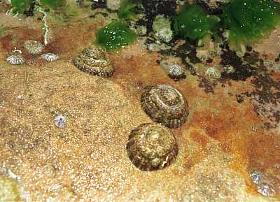
The same marine ecologist that featured earlier was also interested in examining the effects of wave exposure on the abundance of another intertidal marine limpet Cellana tramoserica on rocky intertidal shores. Again, a single quadrat was placed on 10 exposed (to large waves) shores and 10 sheltered shores. From each quadrat, the number of smooth limpets (Cellana tramoserica) were counted.

Download LimpetsSmooth data set

Format of limpetsSmooth.csv data files
Count Shore 4 sheltered 1 sheltered 2 sheltered 0 sheltered 4 sheltered ... ... Shore Categorical description of the shore type (sheltered or exposed) - Predictor variable Count Number of limpets per quadrat - Response variable

Open the limpetsSmooth data set.

> limpets <- read.table("../downloads/data/limpetsSmooth.csv", header = T,
+     sep = ",", strip.white = T)
> limpets
   Count     Shore
1      3 sheltered
2      1 sheltered
3      6 sheltered
4      0 sheltered
5      4 sheltered
6      3 sheltered
7      8 sheltered
8      1 sheltered
9     13 sheltered
10     0 sheltered
11     2   exposed
12    14   exposed
13     2   exposed
14     3   exposed
15    31   exposed
16     1   exposed
17    13   exposed
18     8   exposed
19    14   exposed
20    11   exposed

> limpets.glm <- glm(Count ~ Shore, family = poisson, data = limpets)

1. Check the model for lack of fit via:
   • Pearson Χ²
     Show code

     > limpets.resid <- sum(resid(limpets.glm, type = "pearson")^2)
     > 1 - pchisq(limpets.resid, limpets.glm$df.resid)
     [1] 4.441e-16
     > #Evidence of a lack of fit
     

   • Deviance (G²)
     Show code

     > 1 - pchisq(limpets.glm$deviance, limpets.glm$df.resid)
     [1] 1.887e-15
     > #Evidence of a lack of fit
     

   • Standardized residuals (plot)
     Show code

     > plot(limpets.glm)
     
     
     
     
     

2. Estimate the dispersion parameter to evaluate over dispersion in the fitted model
   • Via Pearson residuals
     Show code

     > limpets.resid/limpets.glm$df.resid
     [1] 6.358
     > #Evidence of over dispersion
     

   • Via deviance
     Show code

     > limpets.glm$deviance/limpets.glm$df.resid
     [1] 6.178
     > #Evidence of over dispersion
     

3. Compare the expected number of zeros to the actual number of zeros to determine whether the model might be zero inflated.
   • Calculate the proportion of zeros in the data
     Show code

     > limpets.tab <- table(limpets$Count == 0)
     > limpets.tab/sum(limpets.tab)
     
     FALSE  TRUE 
       0.9   0.1 
     

   • Now work out the proportion of zeros we would expect from a Poisson distribution with a lambda equal to the mean count of limpets in this study.
     Show code

     > limpets.mu <- mean(limpets$Count)
     > cnts <- rpois(1000, limpets.mu)
     > limpets.tab <- table(cnts == 0)
     > limpets.tab/sum(limpets.tab)
     
     FALSE  TRUE 
     0.999 0.001 
     

     There is a suggestion that there are more zeros than we should expect given the means of each population. It may be that these data are zero inflated, however, given that our other diagnostics have suggested that the model itself might be inappropriate, zero inflation is not the primary concern.

Clearly there is an issue of with overdispersion. There are multiple potential reasons for this. It could be that there are major sources of variability that are not captured within the sampling design. Alternatively it could be that the data are very clumped. For example, often species abundances are clumped - individuals are either not present, or else when they are present they occur in groups.

1. Explore the distribution of counts from each population
   Show code

   > boxplot(Count ~ Shore, data = limpets)
   > rug(jitter(limpets$Count), side = 2)
   
   

1. Fit the model with a quasipoisson distribution in which the dispersion factor (lambda) is not assumed to be 1. The degree of variability (and how this differs from the mean) is estimated and the dispersion factor is incorporated.
   Show code

   > limpets.glmQ <- glm(Count ~ Shore, family = quasipoisson, data = limpets)
   

   1. t-tests
   Show code

   > summary(limpets.glmQ)
   
   Call:
   glm(formula = Count ~ Shore, family = quasipoisson, data = limpets)
   
   Deviance Residuals: 
      Min      1Q  Median      3Q     Max  
   -3.635  -2.630  -0.475   1.045   5.345  
   
   Coefficients:
                  Estimate Std. Error t value Pr(>|t|)    
   (Intercept)       2.293      0.253    9.05  4.1e-08 ***
   Shoresheltered   -0.932      0.477   -1.95    0.066 .  
   ---
   Signif. codes:  0 '***' 0.001 '**' 0.01 '*' 0.05 '.' 0.1 ' ' 1 
   
   (Dispersion parameter for quasipoisson family taken to be 6.358)
   
       Null deviance: 138.18  on 19  degrees of freedom
   Residual deviance: 111.20  on 18  degrees of freedom
   AIC: NA
   
   Number of Fisher Scoring iterations: 5
   
   

   2. Wald F-test. Note that F = t²
   Show code

   > library(car)
   > Anova(limpets.glmQ, test.statistic = "F")
   Analysis of Deviance Table (Type II tests)
   
   Response: Count
              SS Df    F Pr(>F)  
   Shore      27  1 4.24  0.054 .
   Residuals 114 18              
   ---
   Signif. codes:  0 '***' 0.001 '**' 0.01 '*' 0.05 '.' 0.1 ' ' 1 
   > #OR
   > anova(limpets.glmQ, test = "F")
   Analysis of Deviance Table
   
   Model: quasipoisson, link: log
   
   Response: Count
   
   Terms added sequentially (first to last)
   
   
         Df Deviance Resid. Df Resid. Dev    F Pr(>F)  
   NULL                     19        138              
   Shore  1       27        18        111 4.24  0.054 .
   ---
   Signif. codes:  0 '***' 0.001 '**' 0.01 '*' 0.05 '.' 0.1 ' ' 1 
   

2. Fit the model with a negative binomial distribution (which accounts for the clumping).
   Show code

   > limpets.glmNB <- glm.nb(Count ~ Shore, data = limpets)
   

   Check the fit
   Show code

   > limpets.resid <- sum(resid(limpets.glmNB, type = "pearson")^2)
   > 1 - pchisq(limpets.resid, limpets.glmNB$df.resid)
   [1] 0.4334
   > #Deviance
   > 1 - pchisq(limpets.glmNB$deviance, limpets.glmNB$df.resid)
   [1] 0.2155
   

   1. Wald z-tests (these are equivalent to t-tests)
   Show code

   > summary(limpets.glmNB)
   
   Call:
   glm.nb(formula = Count ~ Shore, data = limpets, init.theta = 1.283382111, 
       link = log)
   
   Deviance Residuals: 
      Min      1Q  Median      3Q     Max  
   -1.893  -1.093  -0.231   0.394   1.532  
   
   Coefficients:
                  Estimate Std. Error z value Pr(>|z|)    
   (Intercept)       2.293      0.297    7.73  1.1e-14 ***
   Shoresheltered   -0.932      0.438   -2.13    0.033 *  
   ---
   Signif. codes:  0 '***' 0.001 '**' 0.01 '*' 0.05 '.' 0.1 ' ' 1 
   
   (Dispersion parameter for Negative Binomial(1.283) family taken to be 1)
   
       Null deviance: 26.843  on 19  degrees of freedom
   Residual deviance: 22.382  on 18  degrees of freedom
   AIC: 122
   
   Number of Fisher Scoring iterations: 1
   
   
                 Theta:  1.283 
             Std. Err.:  0.506 
   
    2 x log-likelihood:  -116.018 
   

   2. Wald Chisq-test. Note that Chisq = z²
   Show code

   > library(car)
   > Anova(limpets.glmNB, test.statistic = "Wald")
   Analysis of Deviance Table (Type II tests)
   
   Response: Count
             Df Chisq Pr(>Chisq)  
   Shore      1  4.53      0.033 *
   Residuals 18                   
   ---
   Signif. codes:  0 '***' 0.001 '**' 0.01 '*' 0.05 '.' 0.1 ' ' 1 
   > anova(limpets.glmNB, test = "F")
   Analysis of Deviance Table
   
   Model: Negative Binomial(1.283), link: log
   
   Response: Count
   
   Terms added sequentially (first to last)
   
   
         Df Deviance Resid. Df Resid. Dev    F Pr(>F)  
   NULL                     19       26.8              
   Shore  1     4.46        18       22.4 4.46  0.035 *
   ---
   Signif. codes:  0 '***' 0.001 '**' 0.01 '*' 0.05 '.' 0.1 ' ' 1 
   > anova(limpets.glmNB, test = "Chisq")
   Analysis of Deviance Table
   
   Model: Negative Binomial(1.283), link: log
   
   Response: Count
   
   Terms added sequentially (first to last)
   
   
         Df Deviance Resid. Df Resid. Dev Pr(>Chi)  
   NULL                     19       26.8           
   Shore  1     4.46        18       22.4    0.035 *
   ---
   Signif. codes:  0 '***' 0.001 '**' 0.01 '*' 0.05 '.' 0.1 ' ' 1 
   

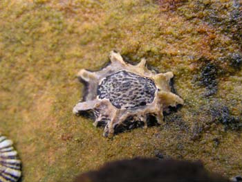
Yet again our rather fixated marine ecologist has returned to the rocky shore with an interest in examining the effects of wave exposure on the abundance of yet another intertidal marine limpet Patelloida latistrigata on rocky intertidal shores. It would appear that either this ecologist is lazy, is satisfied with the methodology or else suffers from some superstition disorder (that prevents them from deviating too far from a series of tasks), and thus, yet again, a single quadrat was placed on 10 exposed (to large waves) shores and 10 sheltered shores. From each quadrat, the number of scaley limpets (Patelloida latistrigata) were counted. Initially, faculty were mildly interested in the research of this ecologist (although lets be honest, most academics usually only display interest in the work of the other members of their school out of politeness - Oh I did not say that did I?). Nevertheless, after years of attending seminars by this ecologist in which the only difference is the target species, faculty have started to display more disturbing levels of animosity towards our ecologist. In fact, only last week, the members of the school's internal ARC review panel (when presented with yet another wave exposure proposal) were rumored to take great pleasure in concocting up numerous bogus applications involving hedgehogs and balloons just so they could rank our ecologist proposal outside of the top 50 prospects and ... Actually, I may just have digressed!

Download LimpetsScaley data set

Format of limpetsScaley.csv data files
Count Shore 4 sheltered 1 sheltered 2 sheltered 0 sheltered 4 sheltered ... ... Shore Categorical description of the shore type (sheltered or exposed) - Predictor variable Count Number of limpets per quadrat - Response variable

Open the limpetsSmooth data set.

> limpets <- read.table("../downloads/data/limpetsScaley.csv", header = T,
+     sep = ",", strip.white = T)
> limpets
   Count     Shore
1      2 sheltered
2      1 sheltered
3      3 sheltered
4      1 sheltered
5      0 sheltered
6      0 sheltered
7      1 sheltered
8      0 sheltered
9      2 sheltered
10     1 sheltered
11     4   exposed
12     9   exposed
13     3   exposed
14     1   exposed
15     3   exposed
16     0   exposed
17     0   exposed
18     7   exposed
19     8   exposed
20     5   exposed

1. Explore the distribution of counts from each population
   Show code

   > boxplot(Count ~ Shore, data = limpets)
   > rug(jitter(limpets$Count), side = 2)
   
   

2. Compare the expected number of zeros to the actual number of zeros to determine whether the model might be zero inflated.
   • Calculate the proportion of zeros in the data
     Show code

     > limpets.tab <- table(limpets$Count == 0)
     > limpets.tab/sum(limpets.tab)
     
     FALSE  TRUE 
      0.75  0.25 
     

   • Now work out the proportion of zeros we would expect from a Poisson distribution with a lambda equal to the mean count of limpets in this study.
     Show code

     > limpets.mu <- mean(limpets$Count)
     > cnts <- rpois(1000, limpets.mu)
     > limpets.tab <- table(cnts == 0)
     > limpets.tab/sum(limpets.tab)
     
     FALSE  TRUE 
      0.91  0.09 
     

     Clearly there are substantially more zeros than expected so the data are not zero inflated.

> library(pscl)
Classes and Methods for R developed in the
Political Science Computational Laboratory
Department of Political Science
Stanford University
Simon Jackman
hurdle and zeroinfl functions by Achim Zeileis
> limpets.zip <- zeroinfl(Count ~ Shore | 1, dist = "poisson", data = limpets)

1. Check the model for lack of fit via:
   • Pearson Χ²
     Show code

     > limpets.resid <- sum(resid(limpets.zip, type = "pearson")^2)
     > 1 - pchisq(limpets.resid, limpets.zip$df.resid)
     [1] 0.281
     > #No evidence of a lack of fit
     

2. Estimate the dispersion parameter to evaluate over dispersion in the fitted model
   • Via Pearson residuals
     Show code

     > limpets.resid/limpets.zip$df.resid
     [1] 1.169
     > #No evidence of over dispersion
     

1. Wald z-tests (these are equivalent to t-tests)
Show code

> summary(limpets.zip)

Call:
zeroinfl(formula = Count ~ Shore | 1, data = limpets, dist = "poisson")

Pearson residuals:
   Min     1Q Median     3Q    Max 
-1.540 -0.940 -0.047  0.846  1.769 

Count model coefficients (poisson with log link):
               Estimate Std. Error z value Pr(>|z|)    
(Intercept)       1.600      0.162    9.89  < 2e-16 ***
Shoresheltered   -1.381      0.362   -3.82  0.00014 ***

Zero-inflation model coefficients (binomial with logit link):
            Estimate Std. Error z value Pr(>|z|)  
(Intercept)   -1.700      0.757   -2.25    0.025 *
---
Signif. codes:  0 '***' 0.001 '**' 0.01 '*' 0.05 '.' 0.1 ' ' 1 

Number of iterations in BFGS optimization: 13 
Log-likelihood: -37.5 on 3 Df

2. Chisq-test. Note that Chisq = z²
Show code

> library(car)
> Anova(limpets.zip, test.statistic = "Chisq")
Analysis of Deviance Table (Type II tests)

Response: Count
          Df Chisq Pr(>Chisq)    
Shore      1  14.6    0.00014 ***
Residuals 17                     
---
Signif. codes:  0 '***' 0.001 '**' 0.01 '*' 0.05 '.' 0.1 ' ' 1 

3. F-test. Note that Chisq = z²
Show code

> library(car)
> Anova(limpets.zip, test.statistic = "F")
Analysis of Deviance Table (Type II tests)

Response: Count
          Df    F Pr(>F)   
Shore      1 14.6 0.0014 **
Residuals 17               
---
Signif. codes:  0 '***' 0.001 '**' 0.01 '*' 0.05 '.' 0.1 ' ' 1 

Interestingly, did you notice that whilst this particular marine ecologists' imagination for design seems somewhat limited, they clearly have a reasonably large statistical tool bag.