Spread assumed to be equal to mean. (\(\phi = 1\))
Dispersion
Over-dispersion
Sample more varied than expected from its mean
variability due to other unmeasured influences
quasi- model
due to more zeros than expected
zero-inflated model
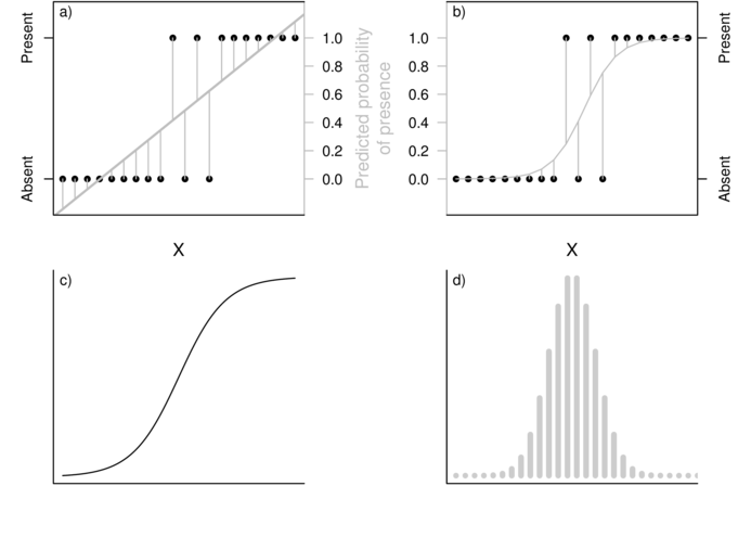
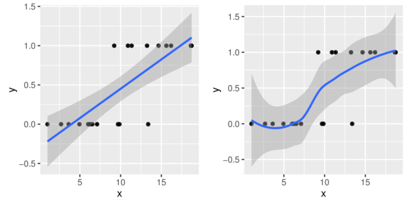
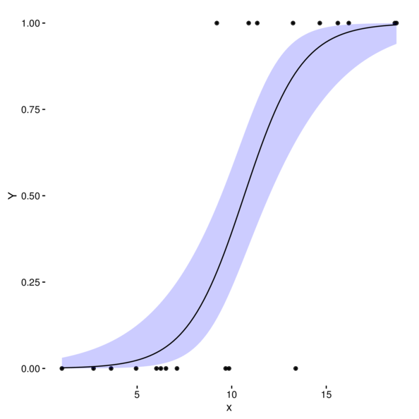
Logistic regression
Example data
  y        x
1 0 1.024733
2 0 2.696719
3 0 3.626263
4 0 4.948643
5 0 6.024718
6 0 6.254113
Logistic regression
Fit model
>dat.glmL <-glm(y ~x, data = dat, family ="binomial")
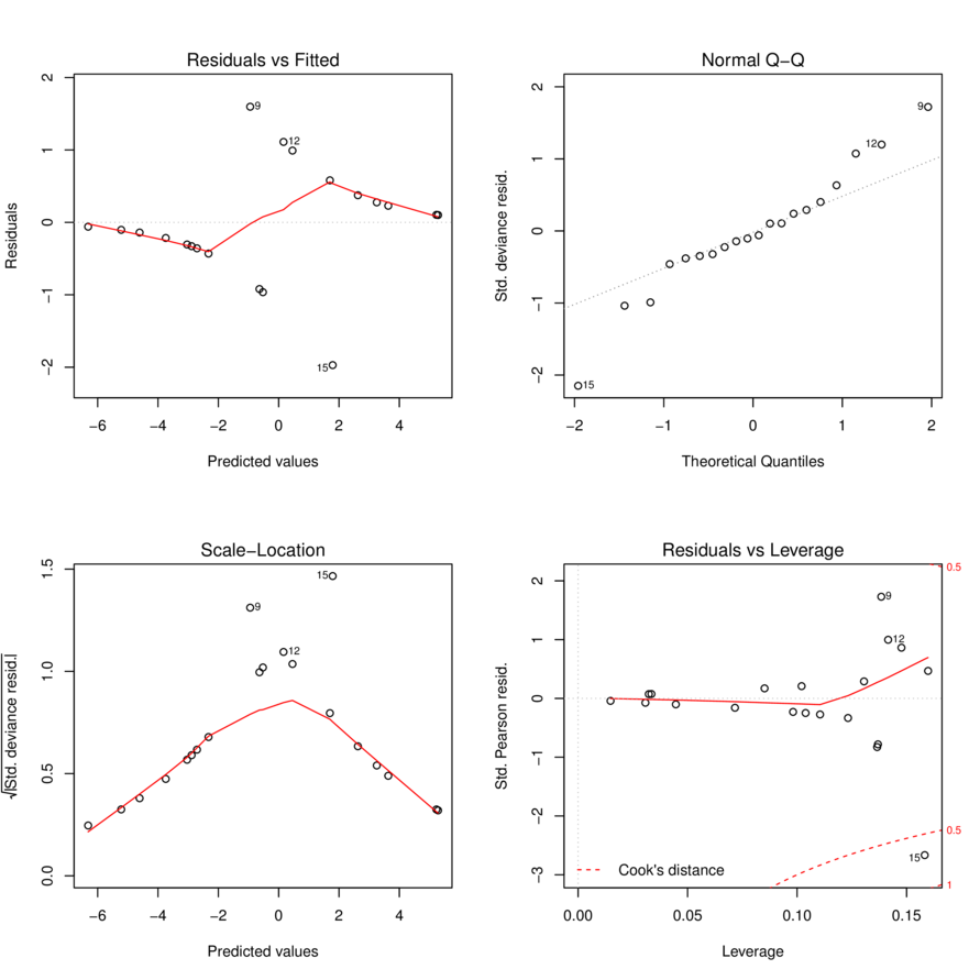
Logistic regression
Explore residuals
>par(mfrow=c(2,2))
>plot(dat.glmL)
Logistic regression
Explore goodness of fit
Pearson’s \(\chi^2\) residuals
>dat.resid <-sum(resid(dat.glmL, type ="pearson")^2)
>1 -pchisq(dat.resid, dat.glmL$df.resid)
[1] 0.8571451
Deviance (\(G^2\))
>1-pchisq(dat.glmL$deviance, dat.glmL$df.resid)
[1] 0.8647024
Logistic regression
Explore model parameters
Slope parameter is on log odds-ratio scale
>summary(dat.glmL)
Call:
glm(formula = y ~ x, family = "binomial", data = dat)

Deviance Residuals:
     Min        1Q    Median        3Q       Max
-1.97157  -0.33665  -0.08191   0.30035   1.59628

Coefficients:
            Estimate Std. Error z value Pr(>|z|)
(Intercept)  -6.9899     3.1599  -2.212   0.0270 *
x             0.6559     0.2936   2.234   0.0255 *
---
Signif. codes:  0 '***' 0.001 '**' 0.01 '*' 0.05 '.' 0.1 ' ' 1

(Dispersion parameter for binomial family taken to be 1)

    Null deviance: 27.526  on 19  degrees of freedom
Residual deviance: 11.651  on 18  degrees of freedom
AIC: 15.651

Number of Fisher Scoring iterations: 6
Logistic regression
Quasi \(R^2\)\[quasi R^2 = 1-\left(\frac{deviance}{null~deviance}\right)\]