Important spatial packages
| Package | Description |
|---|---|
sp |
Defines sp data classes |
maptools |
Routines for reading shapefiles and other mapping data |
mapdata |
Hi-resolution world and regional maps |
raster |
Routines for loading and processing raster data |
rgeos |
A range of spatial manipulation functions |
rgdal |
An R interface to the engine behind complex spatial calculations |
ggplot2 |
Plotting maps |
ggmap |
Google maps |
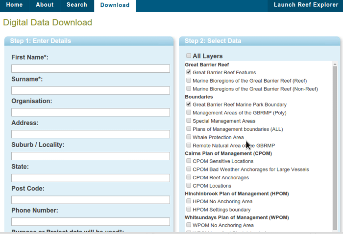
GBRMP shapefiles
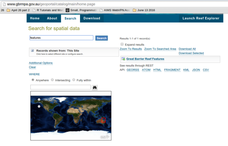
GBRMP shapefiles
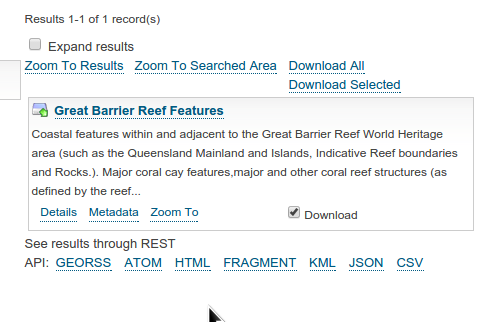
GBRMP shapefiles
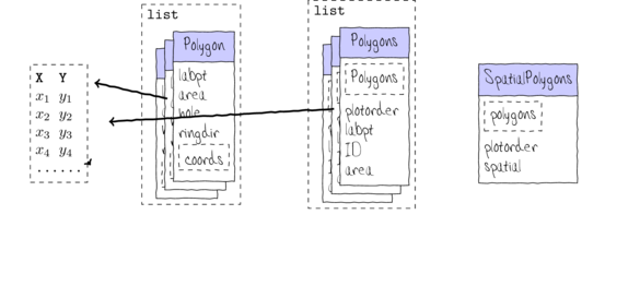
Vectors
Importing spatial data
mapdata - hi-res world maps
> library(mapdata)
> aus <- map("worldHires","Australia", fill=TRUE)
Importing spatial data
mapdata - hi-res world maps
> library(mapdata)
> aus <- map("worldHires","Australia", fill=TRUE, xlim=c(110,160),
+             ylim=c(-45,-5), mar=c(0,0,0,0))
Importing spatial data
mapdata - hi-res world maps
> library(mapdata)
> library(maptools)
> library(sp)
> library(ggplot2)
> aus <- map("worldHires","Australia", fill=TRUE, xlim=c(110,160),
+             ylim=c(-45,-5), mar=c(0,0,0,0), plot=FALSE)
> aus.sp <- map2SpatialPolygons(aus, IDs=aus$names,
+                               proj4string=CRS("+proj=longlat"))
> library(broom)
> ggplot(tidy(aus.sp), aes(y=lat, x=long, group=group)) + geom_polygon()
Importing spatial data
mapdata - hi-res world maps
> ggplot(tidy(aus.sp), aes(y=lat, x=long, group=group)) +
+     geom_polygon(fill='gray60', color='black') +
+     coord_map(xlim=c(146.65,147), ylim=c(-19.35,-19))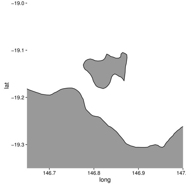
Importing spatial data
mapdata - hi-res world maps
Cropping
> library(rgeos)
> x <- c(146.65,147,147,146.65)
> y <- c(-19.35,-19.35,-19,-19)
> reg=SpatialPolygons(list(Polygons(list(Polygon(cbind(x,y))),ID=1)))
> proj4string(reg) <- CRS('+proj=longlat')
> aus.sp.crop <- gIntersection(aus.sp, reg)
> ggplot(tidy(aus.sp.crop), aes(y=lat, x=long, group=group)) +
+     geom_polygon(fill='gray60', color='black') +
+     coord_map()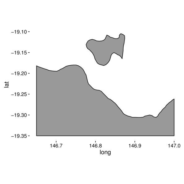
Importing spatial data
Shapefiles
> gbr.sp<- readShapeSpatial(
+     "Great Barrier Reef Features/Great_Barrier_Reef_Features.shp",
+     proj4string = CRS('+proj=longlat +ellps=WGS84'),
+     repair=TRUE,force_ring=T,verbose=TRUE)
> plot(gbr.sp)
Importing spatial data
Shapefiles and ggplot
> gbr.df <- tidy(gbr.sp, region='FEAT_NAME')
> ggplot(gbr.df, aes(y=lat, x=long, fill=id, group=group)) +
+     scale_x_continuous('', expand=c(0,0)) +
+     scale_y_continuous('', expand=c(0,0)) +
+     geom_polygon() + coord_map() + theme_classic() +
+ theme(panel.background=element_rect(fill=NA,color='black')) 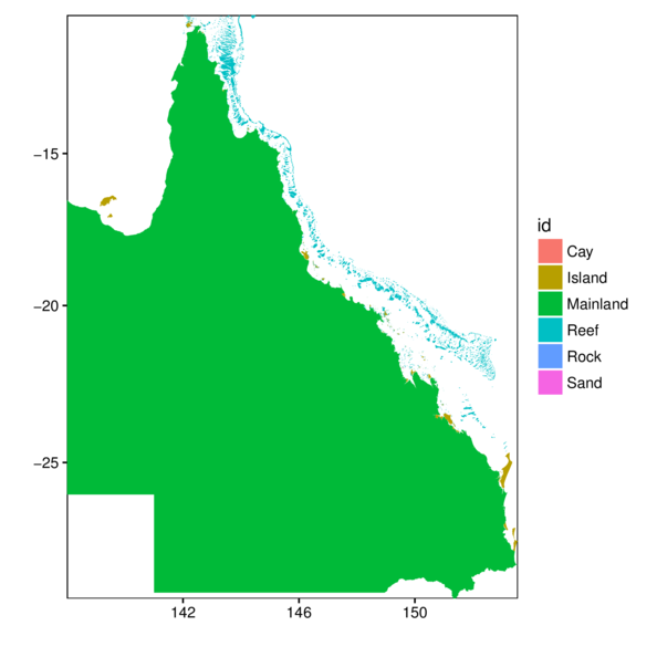
Importing spatial data
Shapefiles - cropping
> #gbr.sp.crop <- gIntersection(gbr.sp, reg, byid=TRUE) # does not honor data frame
> gbr.sp.crop <- raster:::intersect(gbr.sp, reg)
> gbr.tsv.df <- tidy(gbr.sp.crop, region='FEAT_NAME')
> ggplot(gbr.tsv.df, aes(y=lat, x=long, fill=id, group=group)) +
+     scale_x_continuous('', expand=c(0,0)) +
+     scale_y_continuous('', expand=c(0,0)) +
+     geom_polygon() + coord_map() + theme_classic() +
+ theme(panel.background=element_rect(fill=NA,color='black')) 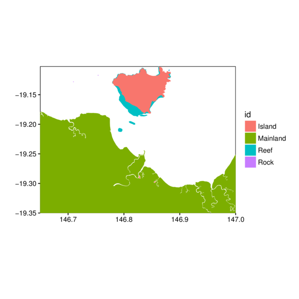
Importing spatial data
Shapefiles - cropping
> ggplot(gbr.tsv.df, aes(y=lat, x=long, fill=id, group=group)) +
+     scale_x_continuous('', expand=c(0,0)) +
+     scale_y_continuous('', expand=c(0,0)) +
+     geom_polygon() + coord_map() + theme_classic() +
+         theme(panel.background=element_rect(fill=NA,color='black'),
+ legend.position=c(0,0), legend.justification=c(0,0)) 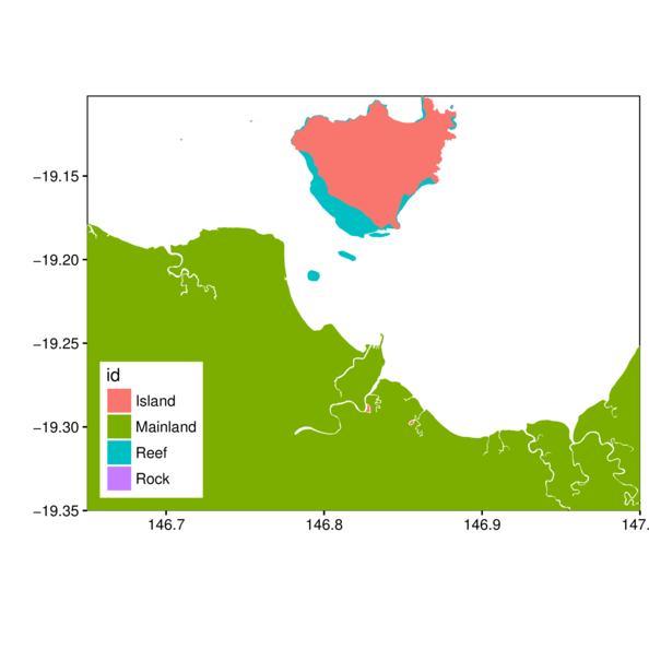
Mapping data
> ggplot(cots, aes(y=Latitude,x=Longitude)) +
+     geom_point() + theme_classic() +
+         theme(panel.background=element_rect(fill=NA, color='black'))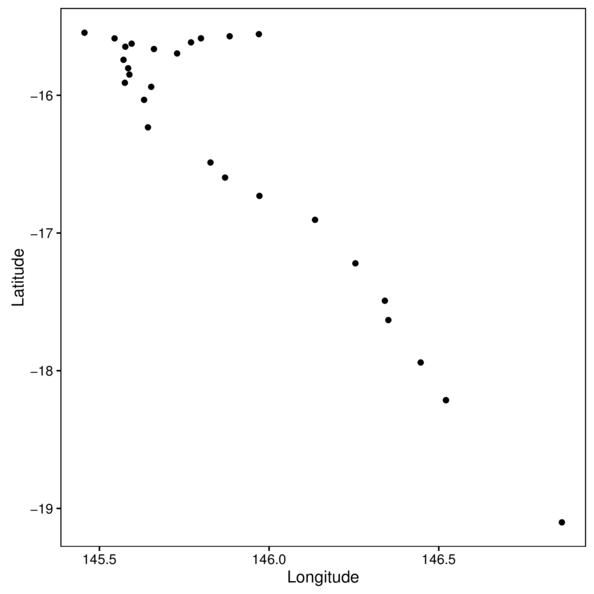
Mapping data
> ggplot(cots, aes(y=Latitude,x=Longitude)) +
+     geom_polygon(data=gbr.df, aes(y=lat, x=long, fill=id, group=group)) +
+     geom_point() + theme_classic() +
+         theme(panel.background=element_rect(fill=NA, color='black'))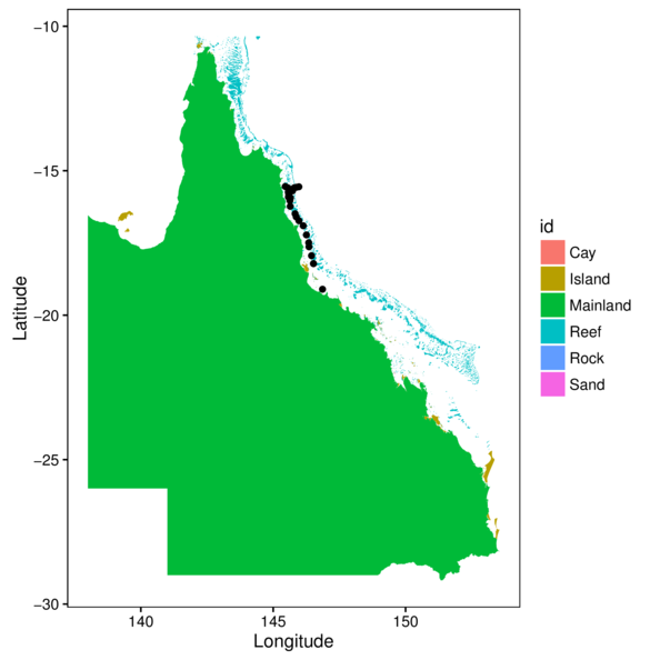
Mapping data
> bb = as(raster:::extent(cbind(cots$Longitude,cots$Latitude))+1,
+     "SpatialPolygons")
> gbr.cots.sp <- raster:::intersect(gbr.sp, bb)
> gbr.cots.df <- tidy(gbr.cots.sp, region='FEAT_NAME')
> ggplot(cots, aes(y=Latitude,x=Longitude)) +
+  geom_polygon(data=gbr.cots.df, aes(y=lat, x=long, fill=id, group=group)) +
+  geom_point() +
+  geom_rect(aes(ymin=-Inf, xmin=-Inf, ymax=Inf, xmax=Inf),
+               fill=NA, color='black')+
+  scale_x_continuous('', expand=c(0,0)) +
+  scale_y_continuous('', expand=c(0,0)) +
+  theme_classic() +
+  theme(legend.position=c(0,0), legend.justification=c(0,0))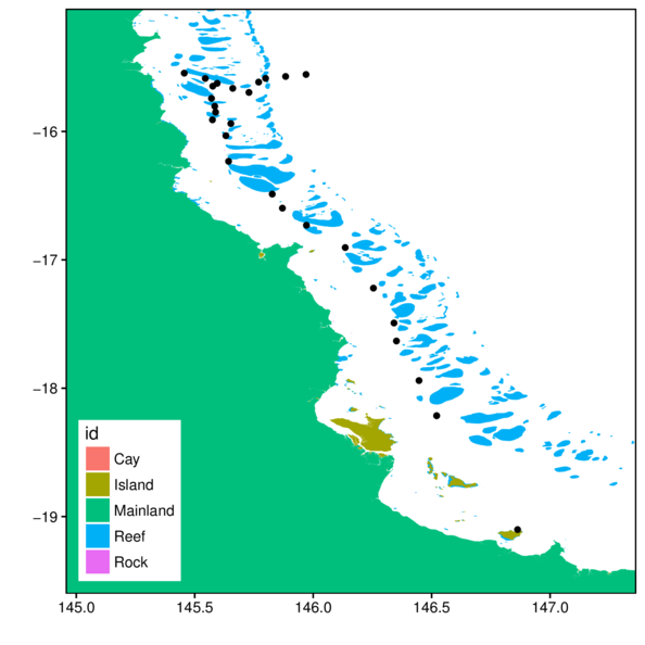
Mapping data
> bb = as(raster:::extent(cbind(cots$Longitude,cots$Latitude))+1,
+     "SpatialPolygons")
> gbr.cots.sp <- raster:::intersect(gbr.sp, bb)
> gbr.cots.df <- tidy(gbr.cots.sp, region='FEAT_NAME')
> ggplot(cots, aes(y=Latitude,x=Longitude)) +
+  geom_polygon(data=gbr.cots.df, aes(y=lat, x=long, fill=id, group=group)) +
+  geom_point() +
+  geom_text(aes(label=Station),hjust=-0.1) +
+  geom_rect(aes(ymin=-Inf, xmin=-Inf, ymax=Inf, xmax=Inf),
+               fill=NA, color='black')+
+  scale_x_continuous('', expand=c(0,0)) +
+  scale_y_continuous('', expand=c(0,0)) +
+  theme_classic() +
+  theme(legend.position=c(0,0), legend.justification=c(0,0))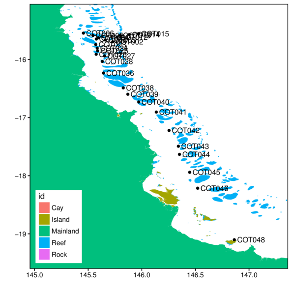
Mapping data
Mapping data
> ggplot(cots, aes(y=Latitude,x=Longitude)) +
+     geom_point(aes(size=Larvae), pch=21) +
+         theme(panel.background=element_rect(fill=NA, color='black'))
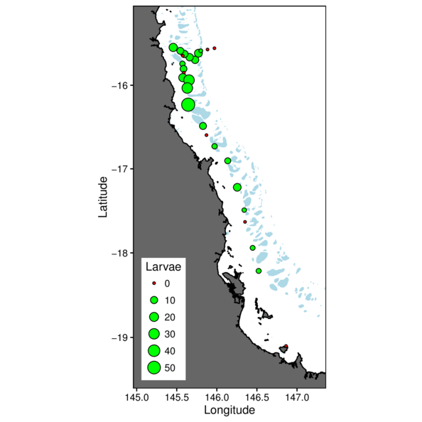
Mapping data
> cots = cots %>% mutate(Present=ifelse(Larvae==0,'N','Y'))
> ggplot(cots, aes(y=Latitude,x=Longitude)) +
+   geom_point(aes(size=Larvae, fill=Present), pch=21) +
+   scale_fill_manual(values=c('red','green'),guide=FALSE)+
+   guides(size=guide_legend(override.aes=list(fill=c('red',rep('green',5))))) +
+   theme(plot.background=element_rect(fill=NA,color='black'),
+         panel.background=element_rect(fill=NA, color='black'),
+ legend.position=c(0,0),legend.justification=c(0,0)) 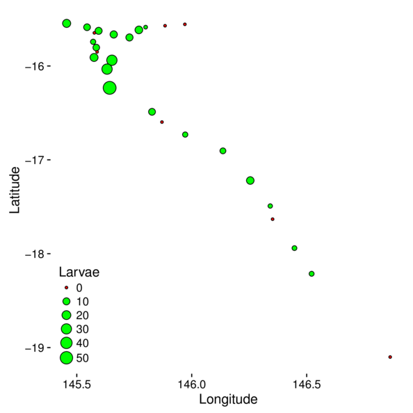
Mapping data
Rasters
> library(ggmap)
> terrain <- get_map(location=c(146,-17.5), zoom=7, maptype="terrain")
> ggmap(terrain) +
+     geom_point(data=cots, aes(y=Latitude,x=Longitude))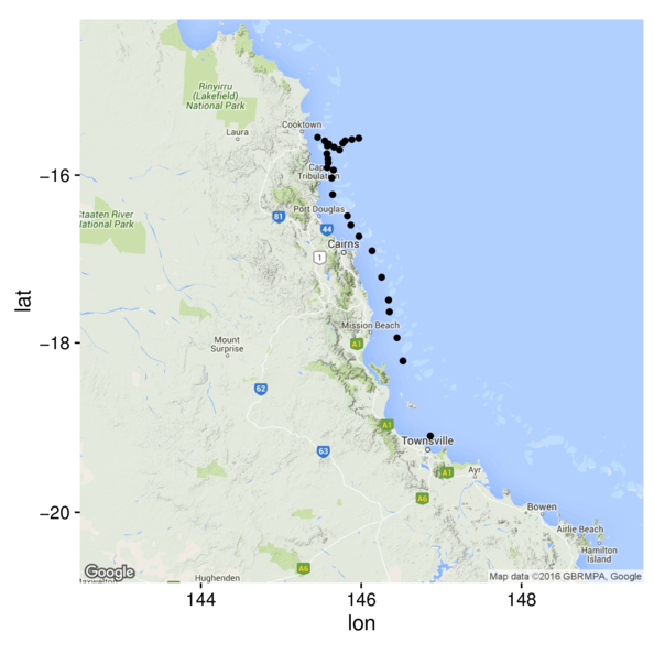
Rasters
> library(ggmap)
> satellite <- get_map(location=c(146,-17.5), zoom=7, maptype="satellite")
> ggmap(satellite) +
+     geom_point(data=cots, aes(y=Latitude,x=Longitude), color='red')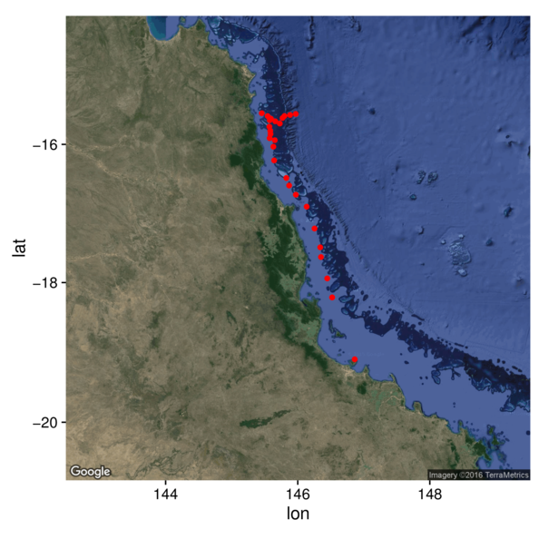
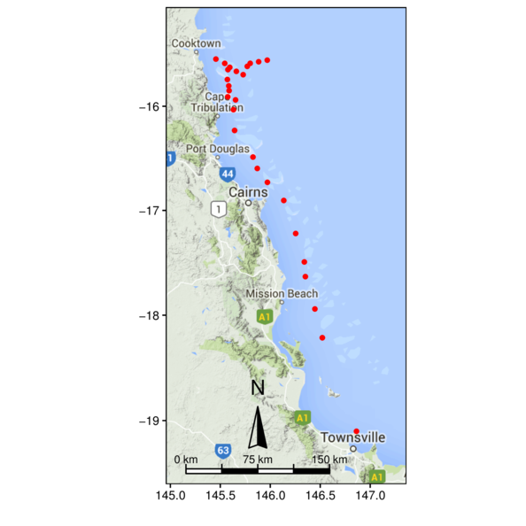
Rasters
> library(ggmap)
> map <- get_googlemap(center=c(146,-17.5), scale=2,zoom=7, maptype="roadmap",
+   style='feature:road|visibility:off&style=element:labels|visibility:off')
> ggmap(map) +
+   geom_point(data=cots, aes(y=Latitude,x=Longitude), color='red')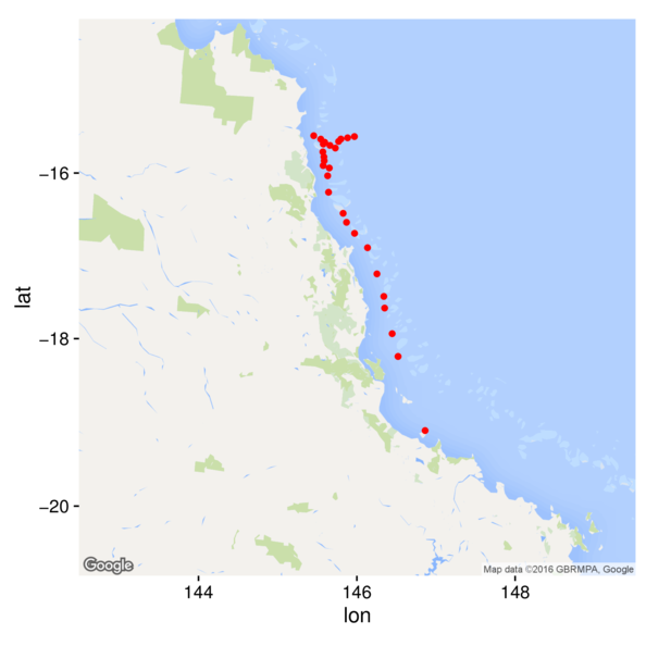
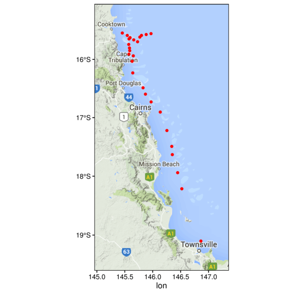
Rasters
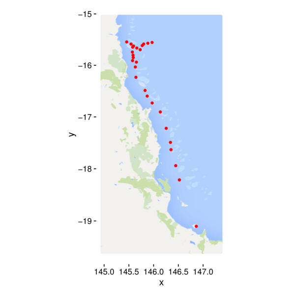
Rasters
> library(ggmap)
> ggmap(terrain) +
+     geom_point(data=cots, aes(y=Latitude,x=Longitude), color='red')+
+         geom_rect(aes(ymin=-Inf, xmin=-Inf, ymax=Inf, xmax=Inf),
+                   fill=NA, color='black')+
+             scale_x_continuous('',expand=c(0,0))+
+                     scale_y_continuous('',expand=c(0,0))+
+             coord_map(xlim=c(144.956, 147.363), ylim=c(-19.601, -15.0455)) +
+                 theme_classic()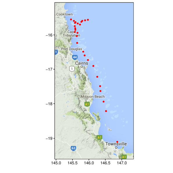
Rasters
Rasters