Aims of statistical modelling

Use samples to:

Describe relationships
Inference testing (relationships/effects)
Predictive models

Mathematical models

A scatterplot of `cars`

Statistical models

A scatterplot of `cars`

Linear models

A scatterplot of `cars`

Linear models

A scatterplot of `cars`

Non-linear models

A scatterplot of `cars`

Linear models

\[ \begin{aligned} y_i &= \qquad\beta_0\qquad + \qquad\beta_1\quad\times \quad x_1 \qquad+ \qquad\epsilon_1\\[1em] \begin{matrix}response\\variable\end{matrix}&= \underbrace{ \underbrace{\begin{matrix}population\\intercept\end{matrix}}_\text{intercept term} \quad + \underbrace{\begin{matrix}population\\slope\end{matrix} \times \begin{matrix}predictor\\variable\end{matrix}}_\text{slope term} }_\text{Systematic component} + \underbrace{error}_\text{Stoichastic component} \end{aligned} \]

Linear models

\[ \begin{aligned} y_i &= \qquad\beta_0\qquad + \qquad\beta_1\quad\times \quad x_1 \qquad+ \qquad\varepsilon_1\\[1em] \begin{matrix}response\\\mathbf{vector}\end{matrix}&= \underbrace{ \underbrace{\begin{matrix}intercept\\\mathbf{single~value}\end{matrix}}_\text{intercept term} \quad + \underbrace{\begin{matrix}slope\\\mathbf{single~value}\end{matrix} \times \begin{matrix}predictor\\\mathbf{vector}\end{matrix}}_\text{slope term} }_\text{Systematic component} + \underbrace{error}_{\text{Stoichastic component}} \end{aligned} \]

Vectors and Matrices

Vector	Matrix
\(\begin{pmatrix}3.0\\2.5\\6.0\\5.5\\9.0\\8.6\\12.0\end{pmatrix}\)	\(\begin{pmatrix}1&0\\1&1\\1&2\\1&3\\1&4\\1&5\\1&6\end{pmatrix}\)
Has length ONLY	Has length AND width

Estimation

A scatterplot of `cars`

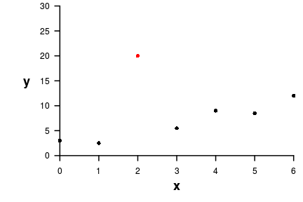
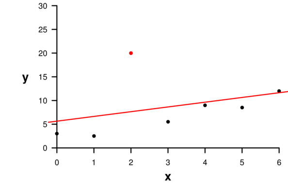
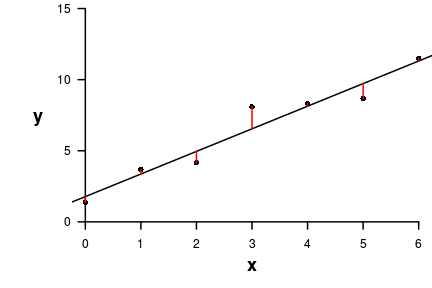
Ordinary Least Squares

Estimation

Y	X
3	0
2.5	1
6	2
5.5	3
9	4
8.6	5
12	6

\[ \begin{alignat*}{4} 3.0\quad&=\quad&\beta_0\times 1\quad&+\quad&\beta_1\times 0\quad&+\quad&\varepsilon_1\\ 2.5\quad&=\quad&\beta_0\times 1\quad&+\quad&\beta_1\times 1\quad&+\quad&\varepsilon_1\\ 6.0\quad&=\quad&\beta_0\times 1\quad&+\quad&\beta_1\times 2\quad&+\quad&\varepsilon_2\\ 5.5\quad&=\quad&\beta_0\times 1\quad&+\quad&\beta_1\times 3\quad&+\quad&\varepsilon_3\\ 9.0\quad&=\quad&\beta_0\times 1\quad&+\quad&\beta_1\times 4\quad&+\quad&\varepsilon_4\\ 8.6\quad&=\quad&\beta_0\times 1\quad&+\quad&\beta_1\times 5\quad&+\quad&\varepsilon_5\\ 12.0\quad&=\quad&\beta_0\times 1\quad&+\quad&\beta_1\times 6\quad&+\quad&\varepsilon_6\\ \end{alignat*} \]

Estimation

\[ \begin{alignat*}{4} 3.0\quad&=\quad&\beta_0\times 1\quad&+\quad&\beta_1\times 0\quad&+\quad&\varepsilon_1\\ 2.5\quad&=\quad&\beta_0\times 1\quad&+\quad&\beta_1\times 1\quad&+\quad&\varepsilon_1\\ 6.0\quad&=\quad&\beta_0\times 1\quad&+\quad&\beta_1\times 2\quad&+\quad&\varepsilon_2\\ 5.5\quad&=\quad&\beta_0\times 1\quad&+\quad&\beta_1\times 3\quad&+\quad&\varepsilon_3\\ 9.0\quad&=\quad&\beta_0\times 1\quad&+\quad&\beta_1\times 4\quad&+\quad&\varepsilon_4\\ 8.6\quad&=\quad&\beta_0\times 1\quad&+\quad&\beta_1\times 5\quad&+\quad&\varepsilon_5\\ 12.0\quad&=\quad&\beta_0\times 1\quad&+\quad&\beta_1\times 6\quad&+\quad&\varepsilon_6\\ \end{alignat*} \]

\[\underbrace{\begin{pmatrix} 3.0\\2.5\\6.0\\5.5\\9.0\\8.6\\12.0 \end{pmatrix}}_\text{Response values} = \underbrace{\begin{pmatrix} 1&0\\1&1\\1&2\\1&3\\1&4\\1&5\\1&6 \end{pmatrix}}_\text{Model matrix} \times \underbrace{\begin{pmatrix} \beta_0\\\beta_1 \end{pmatrix}}_\text{Parameter vector} + \underbrace{\begin{pmatrix} \varepsilon_1\\\varepsilon_2\\\varepsilon_3\\\varepsilon_4&\\\varepsilon_5\\\varepsilon_6 \end{pmatrix}}_\text{Residual vector} \]

Inference testing

Ho:\(\beta_1=0\) (slope equals zero)

The t-statistic

\[t=\frac{param}{SE_{param}}\] \[t=\frac{\beta_1}{SE_{\beta_1}}\]

Inference testing

Ho:\(\beta_1=0\) (slope equals zero)

The t-statistic and the t distribution

Assumptions

Independence - unbiased, scale of treatment
Normality - residuals
Homogeneity of variance - residuals
Linearity

Assumptions

Normality

Assumptions

Homogeneity of variance

Assumptions

Linearity

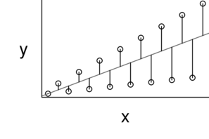
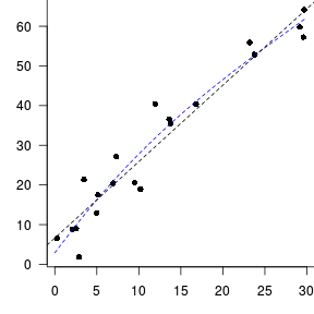
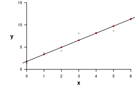
Trendline

Assumptions

Linearity

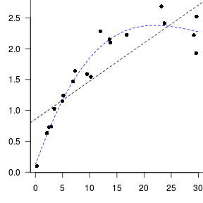
Loess (lowess) smoother

Assumptions

Linearity

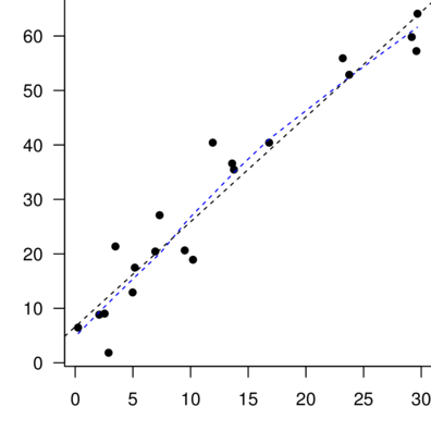
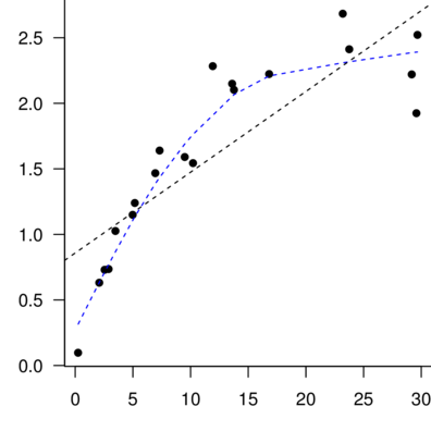
Spline smoother

Assumptions

\[ \begin{align*} y_{i} &= \beta_0 + \beta_1 \times x_{i} + \varepsilon_i\\ \epsilon_i&\sim\mathcal{N}(0, \sigma^2) \\ \end{align*} \]

Assumptions

\[ \begin{align*} y_{i} &= \beta_0 + \beta_1 \times x_{i} + \varepsilon_i\\ \epsilon_i&\sim\mathcal{N}(0, \sigma^2) \\ \end{align*} \]

Example

Make these data and call the data frame DATA

Y	X
3	0
2.5	1
6	2
5.5	3
9	4
8.6	5
12	6

Example

Make these data and call the data frame DATA

Y	X
3	0
2.5	1
6	2
5.5	3
9	4
8.6	5
12	6

try this…

> DATA <- data.frame(Y=c(3, 2.5, 6.0, 5.5, 9.0, 8.6, 12), X=0:6)

Worked Examples

Format of fertilizer.csv data files

FERTILIZER	YIELD
25	84
50	80
75	90
100	154
125	148
…	…

FERTILIZER	Mass of fertilizer (g.m^-2) - Predictor variable
YIELD	Yield of grass (g.m^-2) - Response variable

> fert <- read.csv('../data/fertilizer.csv', strip.white=T)
> fert

   FERTILIZER YIELD
1          25    84
2          50    80
3          75    90
4         100   154
5         125   148
6         150   169
7         175   206
8         200   244
9         225   212
10        250   248

> head(fert)

  FERTILIZER YIELD
1         25    84
2         50    80
3         75    90
4        100   154
5        125   148
6        150   169

> summary(fert)

   FERTILIZER         YIELD      
 Min.   : 25.00   Min.   : 80.0  
 1st Qu.: 81.25   1st Qu.:104.5  
 Median :137.50   Median :161.5  
 Mean   :137.50   Mean   :163.5  
 3rd Qu.:193.75   3rd Qu.:210.5  
 Max.   :250.00   Max.   :248.0

> str(fert)

'data.frame':   10 obs. of  2 variables:
 $ FERTILIZER: int  25 50 75 100 125 150 175 200 225 250
 $ YIELD     : int  84 80 90 154 148 169 206 244 212 248

> library(INLA)
> 
> fert.inla <- inla(YIELD ~ FERTILIZER, data=fert)
> summary(fert.inla)

Call: “inla(formula = YIELD ~ FERTILIZER, data = fert)”

Time used: Pre-processing Running inla Post-processing Total 0.3043 0.0715 0.0217 0.3974

Fixed effects: mean sd 0.025quant 0.5quant 0.975quant mode kld (Intercept) 51.9341 12.9747 25.9582 51.9335 77.8990 51.9339 0 FERTILIZER 0.8114 0.0836 0.6439 0.8114 0.9788 0.8114 0

The model has no random effects

Model hyperparameters: mean sd 0.025quant 0.5quant 0.975quant mode Precision for the Gaussian observations 0.0035 0.0015 0.0012 0.0032 0.007 0.0028

Expected number of effective parameters(std dev): 2.00(0.00) Number of equivalent replicates : 5.00

Marginal log-Likelihood: -61.65

Worked Examples

Question: is there a relationship between fertilizer concentration and grass yeild?

Linear model:

\[ Y_i = \beta_0 + \beta_1 F_i + \varepsilon_i \hspace{1cm} \varepsilon \sim{} \mathcal{N}(0, \sigma^2) \]

Example

Exploratory data analysis

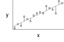
> library(car)
> scatterplot(Y~X, data=DATA)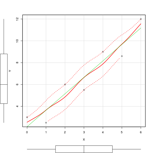

Example

Exploratory data analysis

> library(car)
> peake <- read.csv('../data/peake.csv')
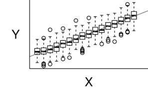
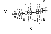
> scatterplot(SPECIES ~ AREA, data=peake)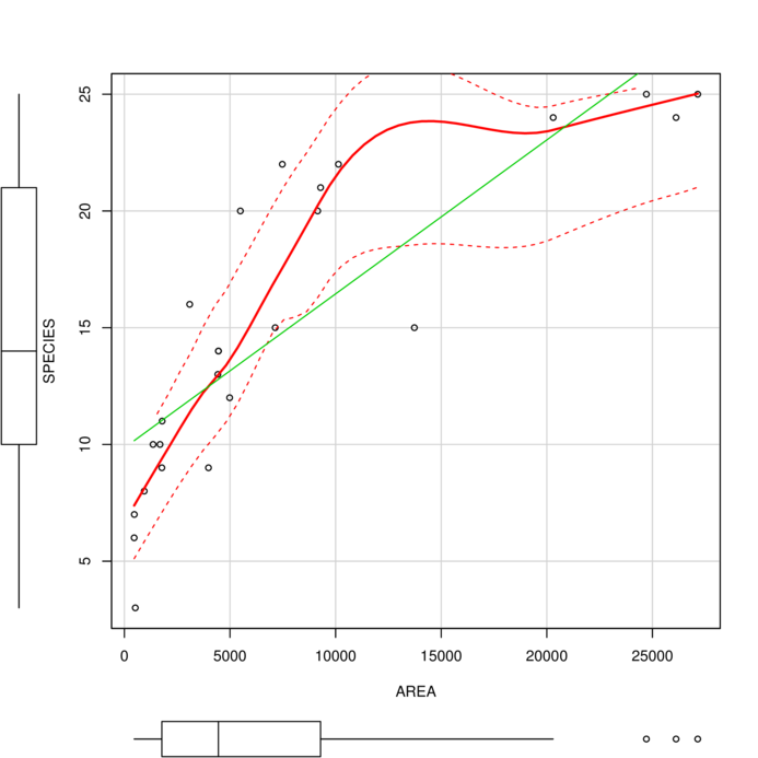

Example

Exploratory data analysis

> scatterplot(SPECIES ~ AREA, data=peake, 
+             smoother=gamLine)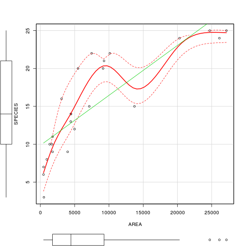

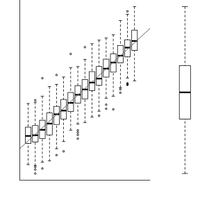
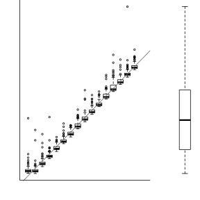
Example

Exploratory data analysis

> library(ggplot2)
> library(gridExtra)
> ggplot(peake, aes(y=SPECIES, x=AREA)) + geom_point()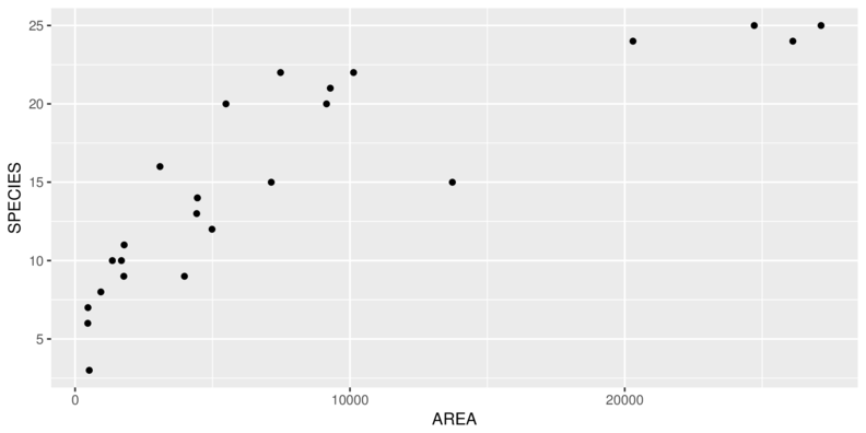

> ggplot(peake, aes(y=SPECIES, x=AREA)) + geom_point() +
+     geom_smooth()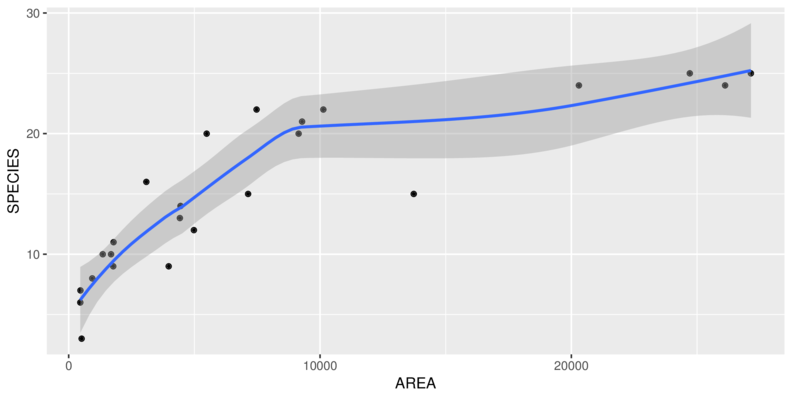

> p2 <- ggplot(peake, aes(y=SPECIES, x=1)) + geom_boxplot()
> p3 <- ggplot(peake, aes(y=AREA, x=1)) + geom_boxplot()
> grid.arrange(p1,p2,p3, ncol=3)

Error in arrangeGrob(...): object 'p1' not found

Linear models in R

> lm(formula, data= DATAFRAME)

Model	R formula	Description
\(y_i = \beta_0 + \beta_1 x_i\)	`y~1+x`
	`y~x`	Full model
\(y_i = \beta_0\)	`y~1`	Null model
\(y_i = \beta_1\)	`y~-1+x`	Through origin

Example

Fit linear model

\[y_i = \beta_0 + \beta_1 x_i \qquad N(0,\sigma)\]

> DATA.lm<-lm(Y~X, data=DATA)

Worked Example

TIME TO FIT A MODEL

Linear models in R

Model diagnostics

Residuals

Model diagnostics

Residuals

Model diagnostics

Leverage

Model diagnostics

Cook’s D

Example

Model evaluation

Extractor	Description
`residuals()`	Extracts residuals from model

> residuals(DATA.lm)

         1          2          3          4          5          6          7 
 0.8642857 -1.1428571  0.8500000 -1.1571429  0.8357143 -1.0714286  0.8214286

Example

Model evaluation

Extractor	Description
`residuals()`	Extracts residuals from model
`fitted()`	Extracts the predicted values

> fitted(DATA.lm)

        1         2         3         4         5         6         7 
 2.135714  3.642857  5.150000  6.657143  8.164286  9.671429 11.178571

Example

Model evaluation

Extractor	Description
`residuals()`	Extracts residuals from model
`fitted()`	Extracts the predicted values
`plot()`	Series of diagnostic plots

> plot(DATA.lm)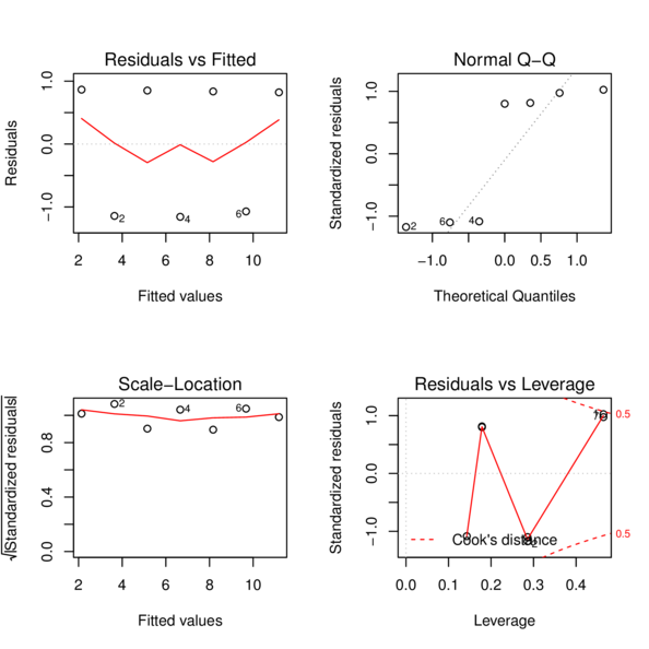

Example

Model evaluation

Extractor	Description
`residuals()`	Residuals
`fitted()`	Predicted values
`plot()`	Diagnostic plots
`influence.measures()`	Leverage (hat) and Cook’s D

Example

Model evaluation

> influence.measures(DATA.lm)

Influence measures of
     lm(formula = Y ~ X, data = DATA) :

   dfb.1_     dfb.X  dffit cov.r cook.d   hat inf
1  0.9603 -7.99e-01  0.960  1.82 0.4553 0.464    
2 -0.7650  5.52e-01 -0.780  1.15 0.2756 0.286    
3  0.3165 -1.63e-01  0.365  1.43 0.0720 0.179    
4 -0.2513 -7.39e-17 -0.453  1.07 0.0981 0.143    
5  0.0443  1.60e-01  0.357  1.45 0.0696 0.179    
6  0.1402 -5.06e-01 -0.715  1.26 0.2422 0.286    
7 -0.3466  7.50e-01  0.901  1.91 0.4113 0.464

Example

Model evaluation

Extractor	Description
`residuals()`	Residuals
`fitted()`	Predicted values
`plot()`	Diagnostic plots
`influence.measures()`	Leverage, Cook’s D
`summary()`	Summarizes important output from model

Example

Model evaluation

> summary(DATA.lm)


Call:
lm(formula = Y ~ X, data = DATA)

Residuals:
      1       2       3       4       5       6       7 
 0.8643 -1.1429  0.8500 -1.1571  0.8357 -1.0714  0.8214 

Coefficients:
            Estimate Std. Error t value Pr(>|t|)    
(Intercept)   2.1357     0.7850   2.721 0.041737 *  
X             1.5071     0.2177   6.923 0.000965 ***
---
Signif. codes:  0 '***' 0.001 '**' 0.01 '*' 0.05 '.' 0.1 ' ' 1

Residual standard error: 1.152 on 5 degrees of freedom
Multiple R-squared:  0.9055,    Adjusted R-squared:  0.8866 
F-statistic: 47.92 on 1 and 5 DF,  p-value: 0.0009648

Example

Model evaluation

Extractor	Description
`residuals()`	Residuals
`fitted()`	Predicted values
`plot()`	Diagnostic plots
`influence.measures()`	Leverage, Cook’s D
`summary()`	Model output
`confint()`	Confidence intervals of parameters

Example

Model evaluation

> confint(DATA.lm)

                2.5 %   97.5 %
(Intercept) 0.1178919 4.153537
X           0.9474996 2.066786

Example

Model evaluation

Extractor	Description
`residuals()`	Residuals
`fitted()`	Predicted values
`plot()`	Diagnostic plots
`influence.measures()`	Leverage, Cook’s D
`summary()`	Model output
`confint()`	Confidence intervals
`predict()`	Predict responses to new levels of predictors

Example

Model evaluation

> predict(DATA.lm, newdata=data.frame(X=c(2.5, 4.1)),
+         se=TRUE)

$fit
       1        2 
5.903571 8.315000 

$se.fit
        1         2 
0.4488222 0.4969340 

$df
[1] 5

$residual.scale
[1] 1.152017

> predict(DATA.lm, newdata=data.frame(X=c(2.5, 4.1)),
+         interval='confidence')

       fit      lwr      upr
1 5.903571 4.749837 7.057306
2 8.315000 7.037591 9.592409

Example

Model evaluation

> predict(DATA.lm, newdata=data.frame(X=c(2.5, 4.1)),
+         interval='prediction')

       fit      lwr       upr
1 5.903571 2.725409  9.081734
2 8.315000 5.089881 11.540119

Prediction

\[\underbrace{\begin{pmatrix} 3.0\\2.5\\6.0\\5.5\\9.0\\8.6\\12.0 \end{pmatrix}}_\text{Response values} = \underbrace{\begin{pmatrix} 1&0\\1&1\\1&2\\1&3\\1&4\\1&5\\1&6 \end{pmatrix}}_\text{Model matrix} \times \underbrace{\begin{pmatrix} \beta_0\\\beta_1 \end{pmatrix}}_\text{Parameter vector} + \underbrace{\begin{pmatrix} \varepsilon_1\\\varepsilon_2\\\varepsilon_3\\\varepsilon_4&\\\varepsilon_5\\\varepsilon_6 \end{pmatrix}}_\text{Residual vector} \]

\[ \underbrace{\begin{pmatrix} 1&0\\1&1\\1&2\\1&3\\1&4\\1&5\\1&6 \end{pmatrix}}_\text{Model matrix} \times \underbrace{\begin{pmatrix} 2.136\\1.507 \end{pmatrix}}_\text{Parameter vector} = \underbrace{\begin{pmatrix} 2.136\\3.643\\5.150\\6.657\\8.164\\9.671\\11.179 \end{pmatrix}}_\text{Predicted values vector} \]

Example

Model evaluation

Extractor	Description
`residuals()`	Residuals
`fitted()`	Predicted values
`plot()`	Diagnostic plots
`influence.measures()`	Leverage, Cook’s D
`summary()`	Model output
`confint()`	Confidence intervals
`predict()`	Predict new responses
`plot(allEffects())`	Effects plots

Example

Model evaluation

> library(effects)
> plot(allEffects(DATA.lm))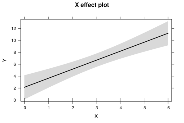

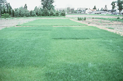
Worked Examples

Format of fertilizer.csv data files

FERTILIZER	YIELD
25	84
50	80
75	90
100	154
125	148
…	…

FERTILIZER	Mass of fertilizer (g.m^-2) - Predictor variable
YIELD	Yield of grass (g.m^-2) - Response variable

> fert <- read.csv('../data/fertilizer.csv', strip.white=T)
> fert

   FERTILIZER YIELD
1          25    84
2          50    80
3          75    90
4         100   154
5         125   148
6         150   169
7         175   206
8         200   244
9         225   212
10        250   248

> head(fert)

  FERTILIZER YIELD
1         25    84
2         50    80
3         75    90
4        100   154
5        125   148
6        150   169

> summary(fert)

   FERTILIZER         YIELD      
 Min.   : 25.00   Min.   : 80.0  
 1st Qu.: 81.25   1st Qu.:104.5  
 Median :137.50   Median :161.5  
 Mean   :137.50   Mean   :163.5  
 3rd Qu.:193.75   3rd Qu.:210.5  
 Max.   :250.00   Max.   :248.0

> str(fert)

'data.frame':   10 obs. of  2 variables:
 $ FERTILIZER: int  25 50 75 100 125 150 175 200 225 250
 $ YIELD     : int  84 80 90 154 148 169 206 244 212 248

Worked Examples

Question: is there a relationship between fertilizer concentration and grass yeild?

Linear model:

\[ Y*i = \beta*0 + \beta_1 F_i + \varepsilon_i \hspace{1cm} \varepsilon \sim{} \mathcal{N}(0, \sigma^2) \]

Worked Examples

Format of peakquinn.csv data files

AREA	INDIV
516.00	18
469.06	60
462.25	57
938.60	100
1357.15	48
…	…

AREA	Area of mussel clump mm² - Predictor variable
INDIV	Number of individuals found within clump - Response variable

> peake <- read.csv('../data/peakquinn.csv', strip.white=T)
> head(peake)

     AREA INDIV
1  516.00    18
2  469.06    60
3  462.25    57
4  938.60   100
5 1357.15    48
6 1773.66   118

> summary(peake)

      AREA             INDIV       
 Min.   :  462.2   Min.   :  18.0  
 1st Qu.: 1773.7   1st Qu.: 148.0  
 Median : 4451.7   Median : 338.0  
 Mean   : 7802.0   Mean   : 446.9  
 3rd Qu.: 9287.7   3rd Qu.: 632.0  
 Max.   :27144.0   Max.   :1402.0

Worked Examples

Question: is there a relationship between mussel clump area and number of individuals?

Linear model:

\[ \begin{align} Indiv_i &= \beta_0 + \beta_1 Area_i + \varepsilon_i \hspace{1cm} &\varepsilon \sim{} \mathcal{N}(0, \sigma^2)\\ ln(Indiv_i) &= \beta_0 + \beta_1 ln(Area_i) + \varepsilon_i \hspace{1cm} &\varepsilon \sim{} \mathcal{N}(0, \sigma^2) \end{align} \]

Workshop 7.2a: Introduction to Linear models

Murray Logan

19 Jul 2017

Revision

Aims of statistical modelling

Mathematical models

Statistical models

Linear models

Linear models

Non-linear models

Linear models

Linear models

Vectors and Matrices

Estimation

Estimation

Estimation

Inference testing

Inference testing

Linear model Assumptions

Assumptions

Assumptions

Normality

Assumptions

Homogeneity of variance

Assumptions

Linearity

Assumptions

Linearity

Assumptions

Linearity

Assumptions

Assumptions

Example

Example

Worked Examples

Worked Examples

Example

Exploratory data analysis

Example

Exploratory data analysis

Example

Exploratory data analysis

Example

Exploratory data analysis

Simple Linear models in R

Linear models in R

Example

Fit linear model

Worked Example

Linear models in R

Model diagnostics

Residuals

Model diagnostics

Residuals

Model diagnostics

Leverage

Model diagnostics

Cook’s D

Example

Model evaluation

Example

Model evaluation

Example

Model evaluation

Example

Model evaluation

Example

Model evaluation

Example

Model evaluation

Example

Model evaluation

Example

Model evaluation

Example

Model evaluation

Example

Model evaluation

Example

Model evaluation