Frequentist vs Bayesian


|
n: 10 |
n: 10 |
n: 100 |
|
n: 10 |
n: 10 |
n: 100 |
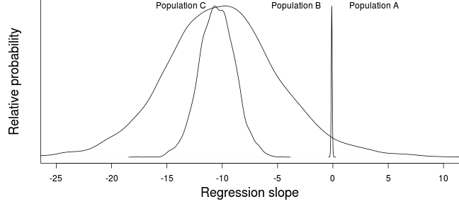
| Population A | Population B | |
|---|---|---|
| Percentage change | 0.46 | 45.46 |
| Prob. >5% decline | 0 | 0.86 |
|
\(P(D\mid H)\) |
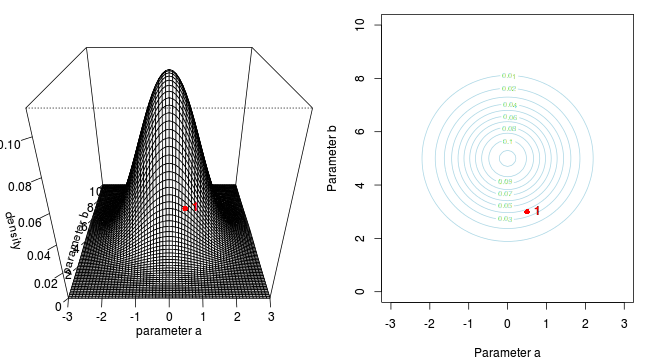
Marchov Chain Monte Carlo sampling
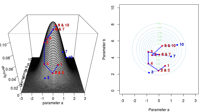
Marchov Chain Monte Carlo sampling
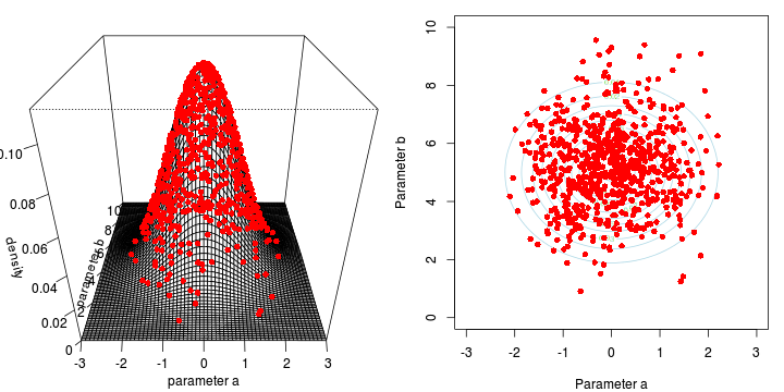
Marchov Chain Monte Carlo sampling

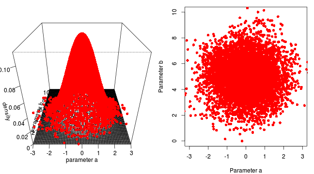
Marchov Chain Monte Carlo sampling
Marchov Chain Monte Carlo sampling
Marchov Chain Monte Carlo sampling

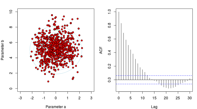
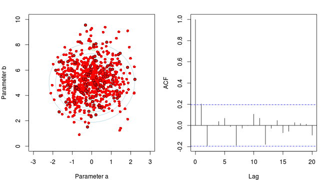
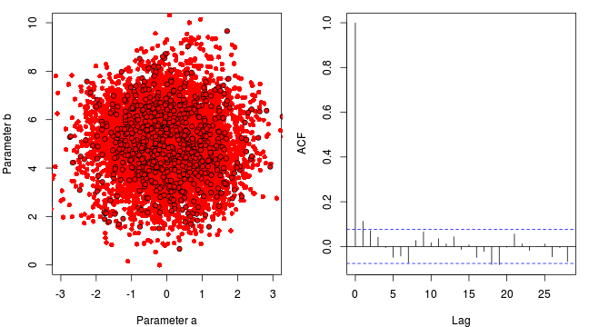
Metropolis-Hastings
http://twiecki.github.io/blog/2014/01/02/visualizing-mcmc/

| Extractor | Description |
|---|---|
residuals() |
Residuals |
fitted() |
Predicted values |
predict() |
Predict new responses |
coef() |
Extract model coefficients |
plot() |
Diagnostic plots |
stanplot(,type=) |
More diagnostic plots |
marginal_effects() |
Partial effects |
logLik() |
Extract log-likelihood |
LOO() and WAIC() |
Calculate WAIC and LOO |
influence.measures() |
Leverage, Cook’s D |
summary() |
Model output |
stancode() |
Model passed to stan |
standata() |
Data list passed to stan |
| Format of fertilizer.csv data files | |||||||||||||||||||
|---|---|---|---|---|---|---|---|---|---|---|---|---|---|---|---|---|---|---|---|
|
|
||||||||||||||||||
> fert <- read.csv('../data/fertilizer.csv', strip.white=T)
> fert
FERTILIZER YIELD
1 25 84
2 50 80
3 75 90
4 100 154
5 125 148
6 150 169
7 175 206
8 200 244
9 225 212
10 250 248> head(fert) FERTILIZER YIELD
1 25 84
2 50 80
3 75 90
4 100 154
5 125 148
6 150 169> summary(fert) FERTILIZER YIELD
Min. : 25.00 Min. : 80.0
1st Qu.: 81.25 1st Qu.:104.5
Median :137.50 Median :161.5
Mean :137.50 Mean :163.5
3rd Qu.:193.75 3rd Qu.:210.5
Max. :250.00 Max. :248.0 > str(fert)'data.frame': 10 obs. of 2 variables:
$ FERTILIZER: int 25 50 75 100 125 150 175 200 225 250
$ YIELD : int 84 80 90 154 148 169 206 244 212 248