Preparations

Packages

library(ggplot2)
library(car)
library(GGally)
library(rstan)
library(brms)
library(coda)
library(dplyr)
library(gridExtra)

Data

Multiple Linear Regression

Additive model

\[growth = intercept + temperature + nitrogen\]

\[y_i=\beta_0+\beta_1x_{i1}+\beta_2x_{i2}+...+\beta_jx_{ij}+\epsilon_i\] OR \[y_i=\beta_0+\sum^N_{j=1:n}{\beta_j x_{ji}}+\epsilon_i\]

Multiple Linear Regression

Additive model

\[growth = intercept + temperature + nitrogen\]

\[y_i=\beta_0+\beta_1x_{i1}+\beta_2x_{i2}+...+\beta_jx_{ij}+\epsilon_i\]
- effect of one predictor holding the other(s) constant

Multiple Linear Regression

Additive model

\(growth = intercept + temperature + nitrogen\)

\(y_i=\beta_0+\beta_1x_{i1}+\beta_2x_{i2}+...+\beta_jx_{ij}+\epsilon_i\)

Multiple Linear Regression

Multiplicative model

\[growth = intercept + temp + nitro + temp\times nitro\]

\[y_i=\beta_0+\beta_1x_{i1}+\beta_2x_{i2}+\beta_3x_{i1}x_{i2}+...+\epsilon_i\]

Assumtions

• normality, homogeneity of variance, linearity
• (multi)collinearity

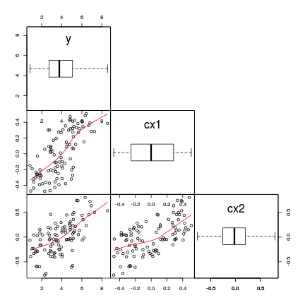
Multiple Linear Regression

Variance inflation

\[ var.inf = \frac{1}{1-R^2} \] Collinear when \(var.inf >= 5\)

Some prefer \(>3\)

Worked examples

Format of loyn.csv data file

ABUND DIST LDIST AREA GRAZE ALT YR.ISOL .. .. .. .. .. .. .. ABUND Abundance of forest birds in patch- response variable DIST Distance to nearest patch - predictor variable LDIST Distance to nearest larger patch - predictor variable AREA Size of the patch - predictor variable GRAZE Grazing intensity (1 to 5, representing light to heavy) - predictor variable ALT Altitude - predictor variable YR.ISOL Number of years since the patch was isolated - predictor variable

loyn <- read.csv('../data/loyn.csv', strip.white=T)
head(loyn)

  ABUND AREA YR.ISOL DIST LDIST GRAZE ALT
1   5.3  0.1    1968   39    39     2 160
2   2.0  0.5    1920  234   234     5  60
3   1.5  0.5    1900  104   311     5 140
4  17.1  1.0    1966   66    66     3 160
5  13.8  1.0    1918  246   246     5 140
6  14.1  1.0    1965  234   285     3 130

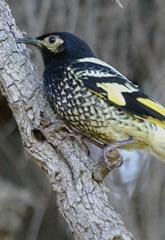
Worked Examples

Question: what effects do fragmentation variables have on the abundance of forest birds

Worked Examples

Format of paruelo.csv data file

C3 LAT LONG MAP JJAMAP DJFMAP .. .. .. .. .. .. C3 Relative abundance of C3 grasses at each site - response variable LAT Latitude in centesimal degrees - predictor variable LONG Longitude in centesimal degrees - predictor variable MAP Mean annual precipitation (mm) - predictor variable MAT Mean annual temperature (0C) - predictor variable JJAMAP Proportion of MAP that fell in June, July and August - predictor variable DJFMAP Proportion of MAP that fell in December, January and Febrary - predictor variable

paruelo <- read.csv('../data/paruelo.csv', strip.white=T)
head(paruelo)

    C3   LAT   LONG MAP  MAT JJAMAP DJFMAP
1 0.65 46.40 119.55 199 12.4   0.12   0.45
2 0.65 47.32 114.27 469  7.5   0.24   0.29
3 0.76 45.78 110.78 536  7.2   0.24   0.20
4 0.75 43.95 101.87 476  8.2   0.35   0.15
5 0.33 46.90 102.82 484  4.8   0.40   0.14
6 0.03 38.87  99.38 623 12.0   0.40   0.11

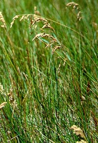
Worked Examples

Question: what effects do fragmentation geographical variables have on the abundance of C3 grasses