41.9
1
48.5
2
43
3
51.4
4
51.2
5
37.7
6
50.7
7
65.1
8
51.7
9
38.9
10
70.6
11
51.4
12
62.7
13
34.9
14
95.3
15
63.9
16
Dealing with Heterogeneity
> data1 <- read.csv ('../data/D1.csv' )
> summary (data1) y x
Min. :34.90 Min. : 1.00
1st Qu.:42.73 1st Qu.: 4.75
Median :51.30 Median : 8.50
Mean :53.68 Mean : 8.50
3rd Qu.:63.00 3rd Qu.:12.25
Max. :95.30 Max. :16.00
\[
\begin{align*}
y_{i} &= \beta_0 + \beta_1 \times x_{i} + \varepsilon_i\\
\epsilon_i&\sim\mathcal{N}(0, \sigma^2) \\
\end{align*}
\]
estimate \(\beta_0\) , \(\beta_1\) and \(\sigma^2\)
Dealing with Heterogeneity
Dealing with Heterogeneity
Dealing with Heterogeneity
\[
\mathbf{V} = cov =
\underbrace{
\begin{pmatrix}
\sigma^2&0&0&0&0&0&0&0&0&0&0&0&0&0&0\\
0&\sigma^2&0&0&0&0&0&0&0&0&0&0&0&0&0\\
0&0&\sigma^2&0&0&0&0&0&0&0&0&0&0&0&0\\
0&0&0&\sigma^2&0&0&0&0&0&0&0&0&0&0&0\\
0&0&0&0&\sigma^2&0&0&0&0&0&0&0&0&0&0\\
0&0&0&0&0&\sigma^2&0&0&0&0&0&0&0&0&0\\
0&0&0&0&0&0&\sigma^2&0&0&0&0&0&0&0&0\\
0&0&0&0&0&0&0&\sigma^2&0&0&0&0&0&0&0\\
0&0&0&0&0&0&0&0&\sigma^2&0&0&0&0&0&0\\
0&0&0&0&0&0&0&0&0&\sigma^2&0&0&0&0&0\\
0&0&0&0&0&0&0&0&0&0&\sigma^2&0&0&0&0\\
0&0&0&0&0&0&0&0&0&0&0&\sigma^2&0&0&0\\
0&0&0&0&0&0&0&0&0&0&0&0&\sigma^2&0&0\\
0&0&0&0&0&0&0&0&0&0&0&0&0&\sigma^2&0\\
0&0&0&0&0&0&0&0&0&0&0&0&0&0&\sigma^2\\
\end{pmatrix}}_\text{Variance-covariance matrix}
\]
Dealing with Heterogeneity
\[
\mathbf{V} = \sigma^2\times
\underbrace{
\begin{pmatrix}
1&0&\cdots&0\\
0&1&\cdots&\vdots\\
\vdots&\cdots&1&\vdots\\
0&\cdots&\cdots&1\\
\end{pmatrix}}_\text{Identity matrix} =
\underbrace{
\begin{pmatrix}
\sigma^2&0&\cdots&0\\
0&\sigma^2&\cdots&\vdots\\
\vdots&\cdots&\sigma^2&\vdots\\
0&\cdots&\cdots&\sigma^2\\
\end{pmatrix}}_\text{Variance-covariance matrix}
\]
Dealing with Heterogeneity
variance proportional to X
variance inversely proportional to X
Dealing with Heterogeneity
variance inversely proportional to X
\[
\mathbf{V} = \sigma^2\times X\times
\underbrace{
\begin{pmatrix}
1&0&\cdots&0\\
0&1&\cdots&\vdots\\
\vdots&\cdots&1&\vdots\\
0&\cdots&\cdots&1\\
\end{pmatrix}}_\text{Identity matrix} =
\underbrace{
\begin{pmatrix}
\sigma^2\times \frac{1}{\sqrt{X_1}}&0&\cdots&0\\
0&\sigma^2\times \frac{1}{\sqrt{X_2}}&\cdots&\vdots\\
\vdots&\cdots&\sigma^2\times \frac{1}{\sqrt{X_i}}&\vdots\\
0&\cdots&\cdots&\sigma^2\times \frac{1}{\sqrt{X_n}}\\
\end{pmatrix}}_\text{Variance-covariance matrix}
\]
Dealing with Heterogeneity
\[
\mathbf{V} = \sigma^2\times \omega, \hspace{1cm} \text{where } \omega =
\underbrace{
\begin{pmatrix}
\frac{1}{\sqrt{X_1}}&0&\cdots&0\\
0&\frac{1}{\sqrt{X_2}}&\cdots&\vdots\\
\vdots&\cdots&\frac{1}{\sqrt{X_i}}&\vdots\\
0&\cdots&\cdots&\frac{1}{\sqrt{X_n}}\\
\end{pmatrix}}_\text{Weights matrix}
\]
Dealing with Heterogeneity
Calculating weights
> 1 /sqrt (data1$x) [1] 1.0000000 0.7071068 0.5773503 0.5000000 0.4472136 0.4082483 0.3779645 0.3535534 0.3333333
[10] 0.3162278 0.3015113 0.2886751 0.2773501 0.2672612 0.2581989 0.2500000
Generalized least squares (GLS)
use OLS to estimate fixed effects
use these estimates to estimate variances via ML
use these to re-estimate fixed effects (OLS)
Generalized least squares (GLS)
ML is biased (for variance) when N is small:
use REML
max. likelihood of residuals rather than data
Variance structures
Variance function
Variance structure
Description
varFixed(~x)
\(V = \sigma^2\times x\)
variance proportional to x the covariate
varExp(form=~x)
\(V = \sigma^2\times e^{2\delta\times x}\)
variance proportional to the exponential of x multiplied by a constant
varPower(form=~x)
\(V = \sigma^2\times |x|^{2\delta}\)
variance proportional to the absolute value of x raised to a constant power
varConstPower(form=~x)
\(V = \sigma^2\times (\delta_1 + |x|^{\delta_2})^2\)
a variant on the power function
varIdent(form=~|A)
\(V = \sigma_j^2\times I\)
when A is a factor, variance is allowed to be different for each level (\(j\) ) of the factor
varComb(form=~x|A)
\(V = \sigma_j^2\times x\times I\)
combination of two of the above
Generalized least squares (GLS)
> library (nlme)
> data1.gls <- gls (y~x, data1,
+ method= 'REML' )
> plot (data1.gls)
> library (nlme)
> data1.gls1 <- gls (y~x, data= data1, weights= varFixed (~x),
+ method= 'REML' )
> plot (data1.gls1)
Generalized least squares (GLS)
> library (nlme)
> data1.gls2 <- gls (y~x, data= data1, weights= varFixed (~x^2 ),
+ method= 'REML' )
> plot (data1.gls2)
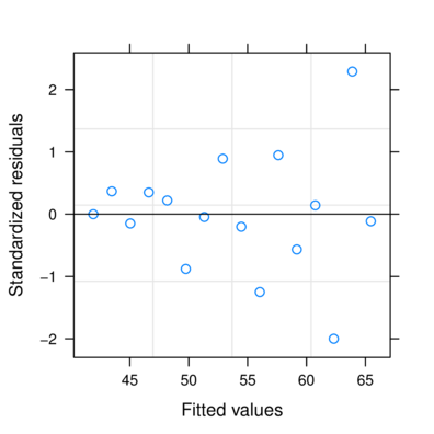
Generalized least squares (GLS)
wrong
> plot (resid (data1.gls) ~
+ fitted (data1.gls))
> plot (resid (data1.gls2) ~
+ fitted (data1.gls2))
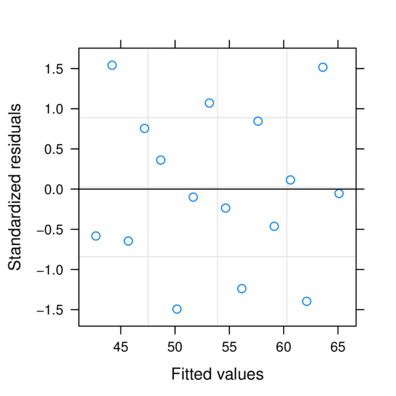
Generalized least squares (GLS)
CORRECT
> plot (resid (data1.gls,'normalized' ) ~
+ fitted (data1.gls))
> plot (resid (data1.gls2,'normalized' ) ~
+ fitted (data1.gls2))
Generalized least squares (GLS)
> plot (resid (data1.gls,'normalized' ) ~ data1$x)
> plot (resid (data1.gls2,'normalized' ) ~ data1$x)
Generalized least squares (GLS)
> AIC (data1.gls, data1.gls1, data1.gls2) df AIC
data1.gls 3 127.6388
data1.gls1 3 121.0828
data1.gls2 3 118.9904> library (MuMIn)
> AICc (data1.gls, data1.gls1, data1.gls2) df AICc
data1.gls 3 129.6388
data1.gls1 3 123.0828
data1.gls2 3 120.9904> #OR
> anova (data1.gls, data1.gls1, data1.gls2) Model df AIC BIC logLik
data1.gls 1 3 127.6388 129.5559 -60.81939
data1.gls1 2 3 121.0828 123.0000 -57.54142
data1.gls2 3 3 118.9904 120.9076 -56.49519
Generalized least squares (GLS)
> summary (data1.gls)Generalized least squares fit by REML
Model: y ~ x
Data: data1
AIC BIC logLik
127.6388 129.5559 -60.81939
Coefficients:
Value Std.Error t-value p-value
(Intercept) 40.33000 7.189442 5.609615 0.0001
x 1.57074 0.743514 2.112582 0.0531
Correlation:
(Intr)
x -0.879
Standardized residuals:
Min Q1 Med Q3 Max
-2.00006105 -0.29319830 -0.02282621 0.35357567 2.29099872
Residual standard error: 13.70973
Degrees of freedom: 16 total; 14 residual
> summary (data1.gls2)Generalized least squares fit by REML
Model: y ~ x
Data: data1
AIC BIC logLik
118.9904 120.9075 -56.49519
Variance function:
Structure: fixed weights
Formula: ~x^2
Coefficients:
Value Std.Error t-value p-value
(Intercept) 41.21920 1.493556 27.598018 0.0000
x 1.49282 0.469988 3.176287 0.0067
Correlation:
(Intr)
x -0.671
Standardized residuals:
Min Q1 Med Q3 Max
-1.49259798 -0.59852829 -0.07669281 0.77799410 1.54157863
Residual standard error: 1.393108
Degrees of freedom: 16 total; 14 residual
Generalized least squares (GLS)
> data1$cx <- scale (data1$x, scale= FALSE )
> data1.gls <- gls (y~cx, data1,
+ method= 'REML' )
> summary (data1.gls)Generalized least squares fit by REML
Model: y ~ cx
Data: data1
AIC BIC logLik
127.6388 129.5559 -60.81939
Coefficients:
Value Std.Error t-value p-value
(Intercept) 53.68125 3.427432 15.662236 0.0000
cx 1.57074 0.743514 2.112582 0.0531
Correlation:
(Intr)
cx 0
Standardized residuals:
Min Q1 Med Q3 Max
-2.00006105 -0.29319830 -0.02282621 0.35357567 2.29099872
Residual standard error: 13.70973
Degrees of freedom: 16 total; 14 residual
> data1$cx <- scale (data1$x, scale= FALSE )
> data1.gls2 <- gls (y~cx, data1,
+ weights= varFixed (~x^2 ), method= 'REML' )
> summary (data1.gls2)Generalized least squares fit by REML
Model: y ~ cx
Data: data1
AIC BIC logLik
118.9904 120.9075 -56.49519
Variance function:
Structure: fixed weights
Formula: ~x^2
Coefficients:
Value Std.Error t-value p-value
(Intercept) 53.90814 3.190165 16.898231 0.0000
cx 1.49282 0.469988 3.176287 0.0067
Correlation:
(Intr)
cx 0.938
Standardized residuals:
Min Q1 Med Q3 Max
-1.49259798 -0.59852829 -0.07669281 0.77799410 1.54157863
Residual standard error: 1.393108
Degrees of freedom: 16 total; 14 residual
Heteroscadacity in ANOVA
> data2 <- read.csv ('../data/D2.csv' )
> summary (data2) y x
Min. :29.29 A:10
1st Qu.:36.17 B:10
Median :40.89 C:10
Mean :42.34 D:10
3rd Qu.:49.32 E:10
Max. :56.84
\[
\begin{align*}
y_{i} &= \mu + \alpha_i + \varepsilon_i\\
\epsilon_i&\sim\mathcal{N}(0, \sigma^2) \\
\end{align*}
\]
estimate \(\mu\) , \(\alpha_i\) and \(\sigma^2\)
Heteroscadacity in ANOVA
> boxplot (y~x, data2)
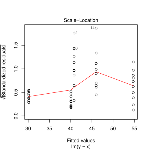
Heteroscadacity in ANOVA
> plot (lm (y~x, data2), which= 3 )
Heteroscadacity in ANOVA
\[\varepsilon \sim \mathcal{N}(0,\sigma_i^2\times \omega)\]
\[\text{Effect (}\alpha\text{) 1 (i=1)} \quad \begin{pmatrix}
y_{1i}\\
y_{2i}\\
y_{3i}\\
\end{pmatrix} =
\begin{pmatrix}
1&1&0&0\\
1&1&0&0\\
1&1&0&0\\
\end{pmatrix} \times
\begin{pmatrix}
\beta_i
\end{pmatrix} +
\begin{pmatrix}
\varepsilon_{1i}\\
\varepsilon_{2i}\\
\varepsilon_{3i}
\end{pmatrix}
\quad
\varepsilon_i \sim \mathcal{N}(0,
\begin{pmatrix}
\sigma_1^2&0&0\\
0&\sigma_1^2&0\\
0&0&\sigma_1^2
\end{pmatrix}
)
\] \[\text{Effect (}\alpha\text{) 2 (i=2)} \quad \begin{pmatrix}
y_{1i}\\
y_{2i}\\
y_{3i}\\
\end{pmatrix} =
\begin{pmatrix}
1&0&1&0\\
1&0&1&0\\
1&0&1&0\\
\end{pmatrix} \times
\begin{pmatrix}
\beta_i
\end{pmatrix} +
\begin{pmatrix}
\varepsilon_{1i}\\
\varepsilon_{2i}\\
\varepsilon_{3i}
\end{pmatrix}
\quad
\varepsilon_i \sim \mathcal{N}(0,
\begin{pmatrix}
\sigma_2^2&0&0\\
0&\sigma_2^2&0\\
0&0&\sigma_2^2
\end{pmatrix}
)
\] \[\text{Effect (}\alpha\text{) 3 (i=3)} \quad \begin{pmatrix}
y_{1i}\\
y_{2i}\\
y_{3i}\\
\end{pmatrix} =
\begin{pmatrix}
1&0&0&1\\
1&0&0&1\\
1&0&0&1\\
\end{pmatrix} \times
\begin{pmatrix}
\beta_i
\end{pmatrix} +
\begin{pmatrix}
\varepsilon_{1i}\\
\varepsilon_{2i}\\
\varepsilon_{3i}
\end{pmatrix}
\quad
\varepsilon_i \sim \mathcal{N}(0,
\begin{pmatrix}
\sigma_3^2&0&0\\
0&\sigma_3^2&0\\
0&0&\sigma_3^2
\end{pmatrix}
)
\]
Heteroscadacity in ANOVA
\[ V_{ji} = \begin{pmatrix}
\sigma_1^2&0&0&0&0&0&0&0&0\\
0&\sigma_1^2&0&0&0&0&0&0&0\\
0&0&\sigma_1^2&0&0&0&0&0&0\\
0&0&0&\sigma_2^2&0&0&0&0&0\\
0&0&0&0&\sigma_2^2&0&0&0&0\\
0&0&0&0&0&\sigma_2^2&0&0&0\\
0&0&0&0&0&0&\sigma_3^2&0&0\\
0&0&0&0&0&0&0&\sigma_3^2&0\\
0&0&0&0&0&0&0&0&\sigma_3^2\\
\end{pmatrix}
\]
Heteroscadacity in ANOVA
> data2.sd <- with (data2, tapply (y,x,sd))
> 1 /(data2.sd[1 ]/data2.sd) A B C D E
1.00000000 0.91342905 0.40807277 0.08632027 0.12720488
Variance structures
Variance function
Variance structure
Description
varFixed(~x)
\(V = \sigma^2\times x\)
variance proportional to x the covariate
varExp(form=~x)
\(V = \sigma^2\times e^{2\delta\times x}\)
variance proportional to the exponential of x multiplied by a constant
varPower(form=~x)
\(V = \sigma^2\times |x|^{2\delta}\)
variance proportional to the absolute value of x raised to a constant power
varConstPower(form=~x)
\(V = \sigma^2\times (\delta_1 + |x|^{\delta_2})^2\)
a variant on the power function
varIdent(form=~|A)
\(V = \sigma_j^2\times I\)
when A is a factor, variance is allowed to be different for each level (\(j\) ) of the factor
varComb(form=~x|A)
\(V = \sigma_j^2\times x\times I\)
combination of two of the above
Heteroscadacity in ANOVA
> library (nlme)
> data2.gls <- gls (y~x, data= data2,
+ method= "REML" )
> library (nlme)
> data2.gls1 <- gls (y~x, data= data2,
+ weights= varIdent (form= ~1 |x), method= "REML" )
Heteroscadacity in ANOVA
> library (nlme)
> data2.gls <- gls (y~x, data= data2,
+ method= "REML" )
> plot (resid (data2.gls,'normalized' ) ~
+ fitted (data2.gls))
> library (nlme)
> data2.gls1 <- gls (y~x, data= data2,
+ weights= varIdent (form= ~1 |x), method= "REML" )
> plot (resid (data2.gls1,'normalized' ) ~
+ fitted (data2.gls1))
Heteroscadacity in ANOVA
> AIC (data2.gls,data2.gls1) df AIC
data2.gls 6 249.4968
data2.gls1 10 199.2087> anova (data2.gls,data2.gls1) Model df AIC BIC logLik Test L.Ratio p-value
data2.gls 1 6 249.4968 260.3368 -118.74841
data2.gls1 2 10 199.2087 217.2753 -89.60435 1 vs 2 58.28812 <.0001
Heteroscadacity in ANOVA
> summary (data2.gls)Generalized least squares fit by REML
Model: y ~ x
Data: data2
AIC BIC logLik
249.4968 260.3368 -118.7484
Coefficients:
Value Std.Error t-value p-value
(Intercept) 40.79322 0.9424249 43.28538 0.0000
xB 5.20216 1.3327901 3.90321 0.0003
xC 13.93944 1.3327901 10.45884 0.0000
xD -0.73285 1.3327901 -0.54986 0.5851
xE -10.65908 1.3327901 -7.99757 0.0000
Correlation:
(Intr) xB xC xD
xB -0.707
xC -0.707 0.500
xD -0.707 0.500 0.500
xE -0.707 0.500 0.500 0.500
Standardized residuals:
Min Q1 Med Q3 Max
-3.30653942 -0.24626108 0.06468242 0.39046918 2.94558782
Residual standard error: 2.980209
Degrees of freedom: 50 total; 45 residual
> summary (data2.gls1)Generalized least squares fit by REML
Model: y ~ x
Data: data2
AIC BIC logLik
199.2087 217.2753 -89.60435
Variance function:
Structure: Different standard deviations per stratum
Formula: ~1 | x
Parameter estimates:
A B C D E
1.00000000 0.91342371 0.40807004 0.08631969 0.12720393
Coefficients:
Value Std.Error t-value p-value
(Intercept) 40.79322 1.481066 27.543153 0.0000
xB 5.20216 2.005924 2.593399 0.0128
xC 13.93944 1.599634 8.714142 0.0000
xD -0.73285 1.486573 -0.492981 0.6244
xE -10.65908 1.493000 -7.139371 0.0000
Correlation:
(Intr) xB xC xD
xB -0.738
xC -0.926 0.684
xD -0.996 0.736 0.922
xE -0.992 0.732 0.918 0.988
Standardized residuals:
Min Q1 Med Q3 Max
-2.3034240 -0.6178652 0.1064904 0.7596732 1.8743230
Residual standard error: 4.683541
Degrees of freedom: 50 total; 45 residual