Compound symmetry

constant correlation (and cov)
sphericity

\[ cor(\varepsilon)= \underbrace{ \begin{pmatrix} 1&\rho&\cdots&\rho\\ \rho&1&\cdots&\vdots\\ \dots&\cdots&1&\vdots\\ \rho&\cdots&\cdots&1\\ \end{pmatrix}}_\text{Correlation matrix} \] \[ \mathbf{V} = \underbrace{ \begin{pmatrix} \theta + \sigma^2&\theta&\cdots&\theta\\ \theta&\theta + \sigma^2&\cdots&\vdots\\ \vdots&\cdots&\theta + \sigma^2&\vdots\\ \theta&\cdots&\cdots&\theta + \sigma^2\\ \end{pmatrix}}_\text{Variance-covariance matrix} \]

Temporal autocorrelation

correlation dependent on proximity
data.t

Temporal autocorrelation

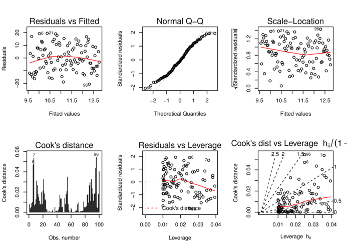
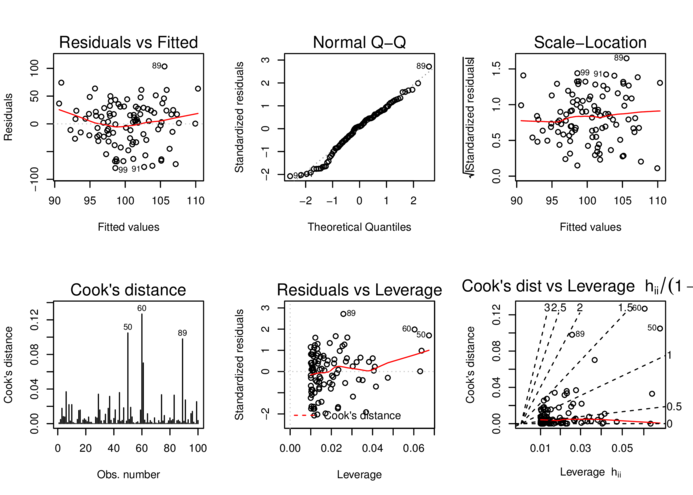
Relationship between Y and X

> data.t.lm <- lm(y~x, data=data.t)
> par(mfrow=c(2,3))
> plot(data.t.lm, which=1:6, ask=FALSE)

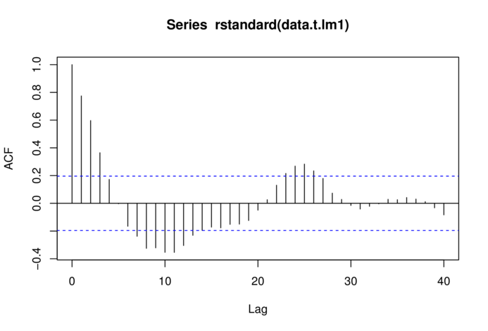
Temporal autocorrelation

Relationship between Y and X

> acf(rstandard(data.t.lm))

Temporal autocorrelation

can we partial out time

> plot(rstandard(data.t.lm)~data.t$year)

Temporal autocorrelation

can we partial out time

> library(car)
> vif(lm(y~x+year, data=data.t))

       x     year 
1.040037 1.040037

> data.t.lm1 <- lm(y~x+year, data.t)

Testing for autocorrelation

Residual plot

> par(mfrow=c(1,2))
> plot(rstandard(data.t.lm1)~fitted(data.t.lm1))
> plot(rstandard(data.t.lm1)~data.t$year)

Testing for autocorrelation

Autocorrelation (acf) plot

> acf(rstandard(data.t.lm1), lag=40)

First order autocorrelation (AR1)

\[ cor(\varepsilon) = \underbrace{ \begin{pmatrix} 1&\rho&\cdots&\rho^{|t-s|}\\ \rho&1&\cdots&\vdots\\ \vdots&\cdots&1&\vdots\\ \rho^{|t-s|}&\cdots&\cdots&1\\ \end{pmatrix}}_\text{First order autoregressive correlation structure} \]

where:

\(s\) and \(t\) are the times.
\(s-t\) is the lag

First order auto-regressive (AR1)

> library(nlme)
> data.t.gls <- gls(y~x+year, data=data.t, method='REML')
> data.t.gls1 <- gls(y~x+year, data=data.t,
+         correlation=corAR1(form=~year),method='REML')

First order auto-regressive (AR1)

> par(mfrow=c(1,2))
> plot(residuals(data.t.gls, type="normalized")~
+      fitted(data.t.gls))
> plot(residuals(data.t.gls1, type="normalized")~
+      fitted(data.t.gls1))

First order auto-regressive (AR1)

> par(mfrow=c(1,2))
> plot(residuals(data.t.gls, type="normalized")~
+      data.t$x)
> plot(residuals(data.t.gls1, type="normalized")~
+      data.t$x)

First order auto-regressive (AR1)

> par(mfrow=c(1,2))
> plot(residuals(data.t.gls, type="normalized")~
+      data.t$year)
> plot(residuals(data.t.gls1, type="normalized")~
+      data.t$year)

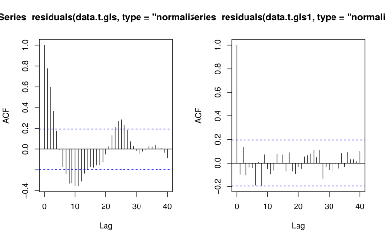
First order auto-regressive (AR1)

> par(mfrow=c(1,2))
> acf(residuals(data.t.gls, type='normalized'), lag=40)
> acf(residuals(data.t.gls1, type='normalized'), lag=40)

First order auto-regressive (AR1)

> AIC(data.t.gls, data.t.gls1)

            df      AIC
data.t.gls   4 626.3283
data.t.gls1  5 536.7467

> anova(data.t.gls, data.t.gls1)

            Model df      AIC      BIC    logLik   Test  L.Ratio p-value
data.t.gls      1  4 626.3283 636.6271 -309.1642                        
data.t.gls1     2  5 536.7467 549.6203 -263.3734 1 vs 2 91.58158  <.0001

Auto-regressive moving average (ARMA)

> data.t.gls2 <- update(data.t.gls,
+    correlation=corARMA(form=~year,p=2,q=0))
> data.t.gls3 <- update(data.t.gls,
+    correlation=corARMA(form=~year,p=3,q=0))
> AIC(data.t.gls, data.t.gls1, data.t.gls2, data.t.gls3)

            df      AIC
data.t.gls   4 626.3283
data.t.gls1  5 536.7467
data.t.gls2  6 538.1032
data.t.gls3  7 538.8376

Summarize model

> summary(data.t.gls1)

Generalized least squares fit by REML
  Model: y ~ x + year 
  Data: data.t 
       AIC      BIC    logLik
  536.7467 549.6203 -263.3734

Correlation Structure: ARMA(1,0)
 Formula: ~year 
 Parameter estimate(s):
     Phi1 
0.9126603 

Coefficients:
               Value Std.Error   t-value p-value
(Intercept) 4388.568 1232.6129  3.560378  0.0006
x              0.028    0.0086  3.296648  0.0014
year          -2.195    0.6189 -3.545955  0.0006

 Correlation: 
     (Intr) x     
x     0.009       
year -1.000 -0.010

Standardized residuals:
      Min        Q1       Med        Q3       Max 
-1.423389  1.710551  3.377925  4.372772  6.624381 

Residual standard error: 3.37516 
Degrees of freedom: 100 total; 97 residual

Spatial autocorrelation

similar, yet dependency is 2d
2d Euclidean dissimilarity
Exponential decay

\[ cor(\varepsilon) = \underbrace{ \begin{pmatrix} 1&e^{-\delta}&\cdots&e^{-\delta D}\\ e^{-\delta}&1&\cdots&\vdots\\ \vdots&\cdots&1&\vdots\\ e^{-\delta D}&\cdots&\cdots&1\\ \end{pmatrix}}_\text{Exponential autoregressive correlation structure} \]

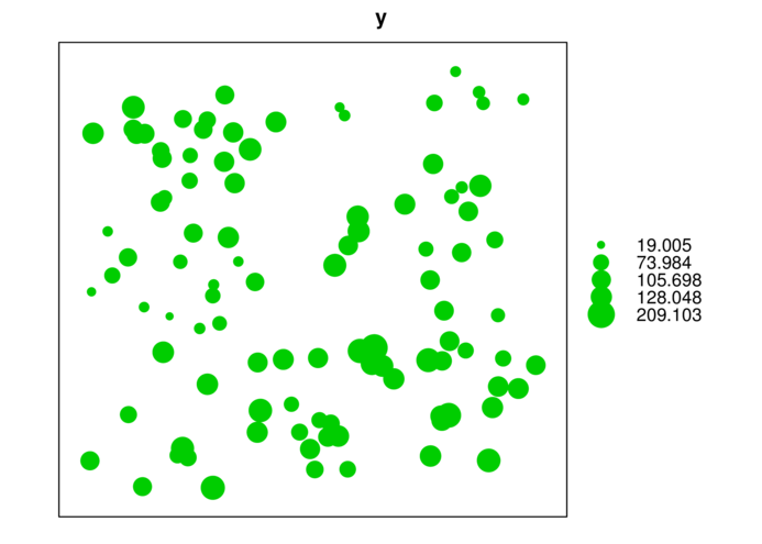
Spatial autocorrelation

data.s

Spatial autocorrelation

Spatial arrangement of Y

> library(sp)
> coordinates(data.s) <- ~LAT+LONG
> bubble(data.s,'y')

Spatial autocorrelation

Relationship between Y and X

> data.s.lm <- lm(y~x, data=data.s)
> par(mfrow=c(2,3))
> plot(data.s.lm, which=1:6, ask=FALSE)

Detecting spatial autocorrelation

bubble plot
semi-variogram

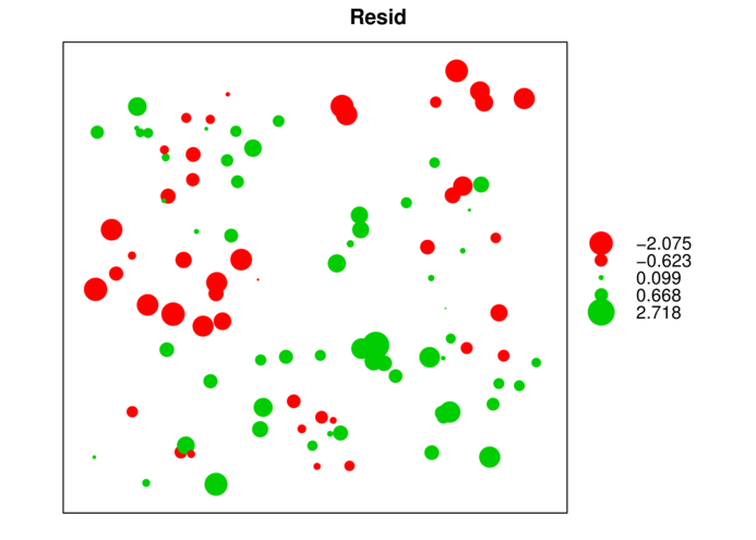
Bubble plot

> data.s$Resid <- rstandard(data.s.lm)
> library(sp)
> #coordinates(data.s) <- ~LAT+LONG
> bubble(data.s,'Resid')

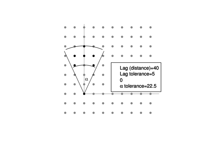
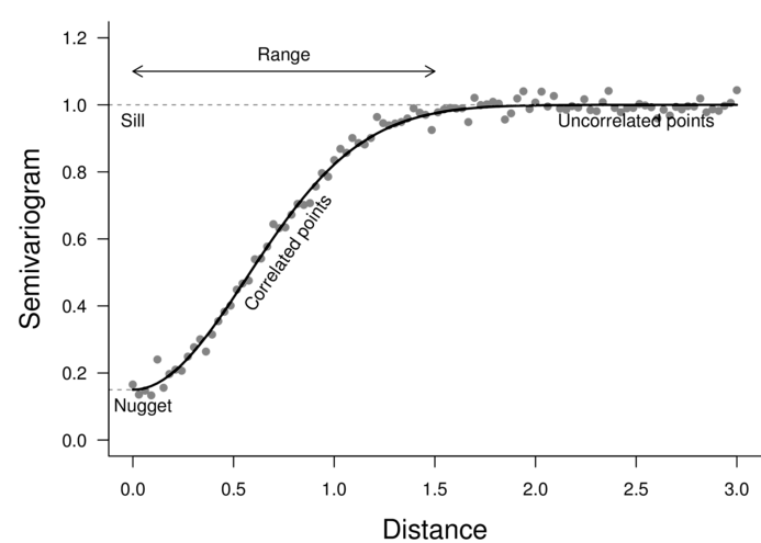
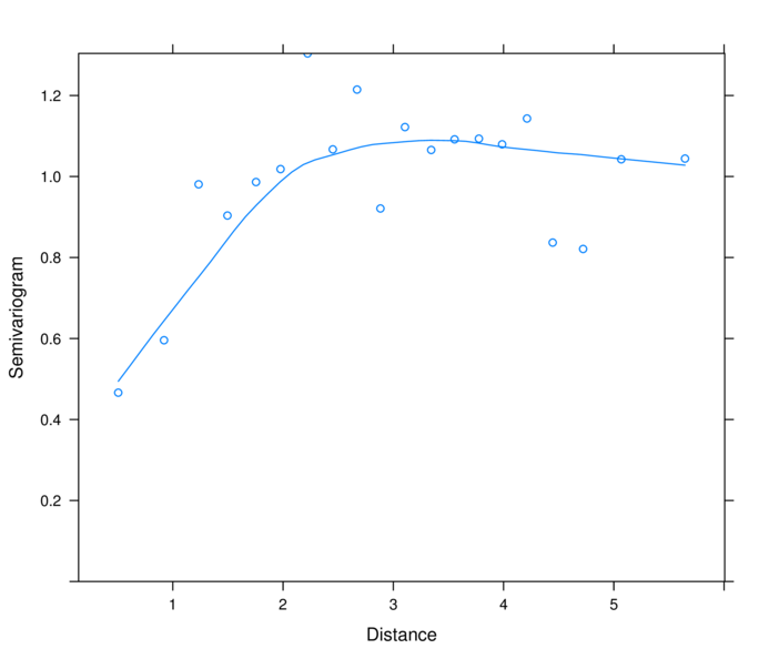
Semi-variogram

semivariance = similarity (of residuals) between pairs at specific distances
distances binned according to distance and orientation (N)

Semi-variogram

> library(nlme)
> data.s.gls <- gls(y~x, data.s, method='REML')
> plot(nlme:::Variogram(data.s.gls, form=~LAT+LONG,
+        resType="normalized"))

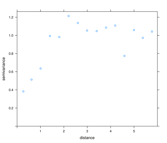
Semi-variogram

> library(gstat)
> plot(variogram(residuals(data.s.gls,"normalized")~1,
+       data=data.s, cutoff=6))

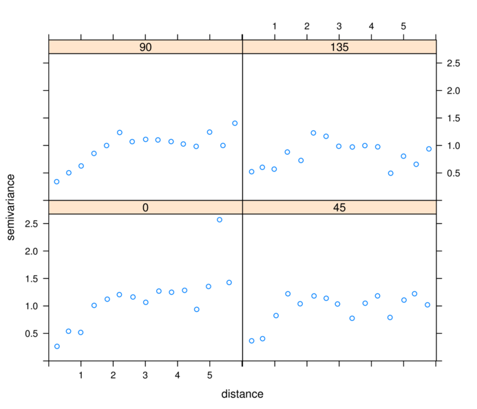
Semi-variogram

> library(gstat)
> plot(variogram(residuals(data.s.gls,"normalized")~1,
+     data=data.s, cutoff=6,alpha=c(0,45,90,135)))

Accommodating spatial autocorrelation

correlation function	Correlation structure	Description
`corExp(form=~lat+long)`	Exponential	\(\Phi = 1-e^{-D/\rho}\)
`corGaus(form=~lat+long)`	Gaussian	\(\Phi = 1-e^{-(D/\rho)^2}\)
`corLin(form=~lat+long)`	Linear	\(\Phi = 1-(1-D/\rho)I(d<\rho)\)
`corRatio(form=~lat+long)`	Rational quadratic	\(\Phi = (d/\rho)^2/(1+(d/\rho)2)\)
`corSpher(form=~lat+long)`	Spherical	\(\Phi = 1-(1-1.5(d/\rho) + 0.5(d/\rho)^3)I(d<\rho)\)

Accommodating spatial autocorrelation

> data.s.glsExp <- update(data.s.gls,
+    correlation=corExp(form=~LAT+LONG, nugget=TRUE))
> data.s.glsGaus <- update(data.s.gls,
+   correlation=corGaus(form=~LAT+LONG, nugget=TRUE))
> #data.s.glsLin <- update(data.s/gls,
> #  correlation=corLin(form=~LAT+LONG, nugget=TRUE))
> data.s.glsRatio <- update(data.s.gls,
+   correlation=corRatio(form=~LAT+LONG, nugget=TRUE))
> data.s.glsSpher <- update(data.s.gls,
+   correlation=corSpher(form=~LAT+LONG, nugget=TRUE))
> 
> AIC(data.s.gls, data.s.glsExp, data.s.glsGaus, data.s.glsRatio, data.s.glsSpher)

                df       AIC
data.s.gls       3 1013.9439
data.s.glsExp    5  974.3235
data.s.glsGaus   5  976.4422
data.s.glsRatio  5  974.7862
data.s.glsSpher  5  975.5244

Accommodating spatial autocorrelation

> plot(residuals(data.s.glsExp, type="normalized")~
+      fitted(data.s.glsExp))

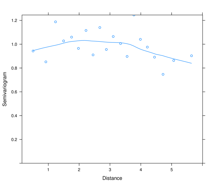
Accommodating spatial autocorrelation

> plot(nlme:::Variogram(data.s.glsExp, form=~LAT+LONG,
+      resType="normalized"))

Summarize model

> summary(data.s.glsExp)

Generalized least squares fit by REML
  Model: y ~ x 
  Data: data.s 
       AIC      BIC    logLik
  974.3235 987.2484 -482.1618

Correlation Structure: Exponential spatial correlation
 Formula: ~LAT + LONG 
 Parameter estimate(s):
    range    nugget 
1.6956723 0.1280655 

Coefficients:
               Value Std.Error  t-value p-value
(Intercept) 65.90018 21.824752 3.019516  0.0032
x            0.94572  0.286245 3.303886  0.0013

 Correlation: 
  (Intr)
x -0.418

Standardized residuals:
       Min         Q1        Med         Q3        Max 
-1.6019483 -0.3507695  0.1608776  0.6451751  2.1331505 

Residual standard error: 47.68716 
Degrees of freedom: 100 total; 98 residual

> anova(data.s.glsExp)

Denom. DF: 98 
            numDF  F-value p-value
(Intercept)     1 23.45923  <.0001
x               1 10.91566  0.0013

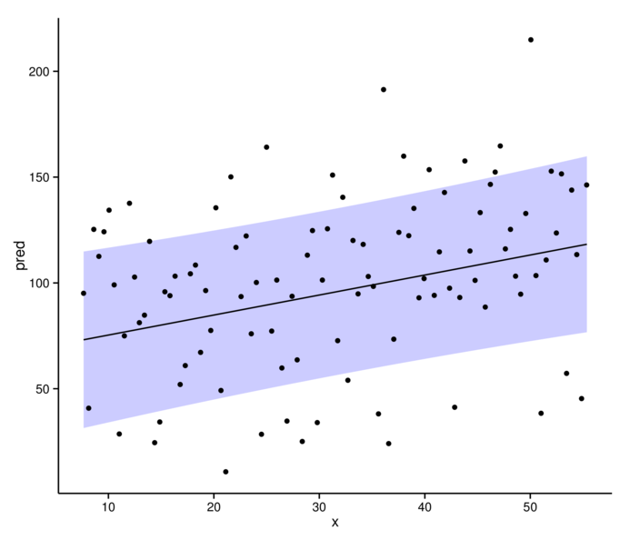
Summarize model

> xs <- seq(min(data.s$x), max(data.s$x), l=100)
> xmat <- model.matrix(~x, data.frame(x=xs))
> 
> mpred <- function(model, xmat, data.s) {
+   pred <- as.vector(coef(model) %*% t(xmat))
+   (se<-sqrt(diag(xmat %*% vcov(model) %*% t(xmat))))
+   ci <- data.frame(pred+outer(se,qt(df=nrow(data.s)-2,c(.025,.975))))
+   colnames(ci) <- c('lwr','upr')
+   data.s.sum<-data.frame(pred, x=xs,se,ci)
+   data.s.sum
+ }
> 
> data.s.sum<-mpred(data.s.glsExp, xmat, data.s)
> data.s.sum$resid <- data.s.sum$pred+residuals(data.s.glsExp)
> 
> library(ggplot2)
> ggplot(data.s.sum, aes(y=pred, x=x))+
+     geom_ribbon(aes(ymin=lwr, ymax=upr), fill='blue', alpha=0.2) +
+     geom_line()+geom_point(aes(y=resid)) + theme_classic()

> #plot(pred~x, ylim=c(min(lwr), max(upr)), data.s.sum, type="l")
> #lines(lwr~x, data.s.sum)
> #lines(upr~x, data.s.sum)
> #points(pred+residuals(data.s.glsExp)~x, data.s.sum)
> 
> #newdata <- data.frame(x=xs)[1,]

Workshop 8.3a: Non-independence part 1

Murray Logan

28 May 2015

Linear modelling assumptions

Linear modelling assumptions

Variance-covariance

Compound symmetry

Temporal autocorrelation

Temporal autocorrelation

Temporal autocorrelation

Temporal autocorrelation

Temporal autocorrelation

Testing for autocorrelation

Residual plot

Testing for autocorrelation

Autocorrelation (acf) plot

First order autocorrelation (AR1)

First order auto-regressive (AR1)

First order auto-regressive (AR1)

First order auto-regressive (AR1)

First order auto-regressive (AR1)

First order auto-regressive (AR1)

First order auto-regressive (AR1)

Auto-regressive moving average (ARMA)

Summarize model

Spatial autocorrelation

Spatial autocorrelation

Spatial autocorrelation

Spatial autocorrelation

Spatial autocorrelation

Detecting spatial autocorrelation

Bubble plot

Semi-variogram

Semi-variogram

Semi-variogram

Semi-variogram

Semi-variogram

Accommodating spatial autocorrelation

Accommodating spatial autocorrelation

Accommodating spatial autocorrelation

Accommodating spatial autocorrelation

Summarize model

Summarize model

Summarize model