Linear models

How maximize power?

Linear models

How maximize power?

increase replication
add covariates (account for conditions)
block (control conditions)

Hierarchical models

To increase power - without more sites (replicates)

Hierarchical models

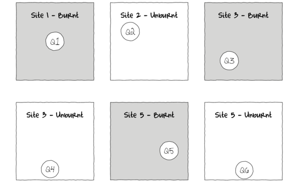
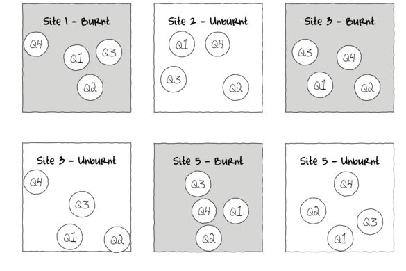
Subreplicates - yet not independent

Hierarchical models

Nested design

Hierarchical models

Nested design

Hierarchical models

Nested design

Hierarchical models

To increase power…

Hierarchical models

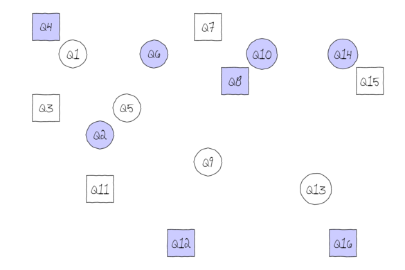
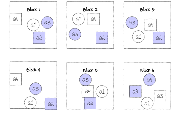
Block treatments together - yet not independent

Hierarchical models

Randomized complete block

Hierarchical models

Randomized complete block

Hierarchical models

Randomized complete block

Linear modelling assumptions

Normality
Homogeneity of Variance
Linearity
Independence

Non-independence

one response is triggered by another
temporal/spatial autocorrelation
nested (hierarchical) design structures

Hierarchical models

linear model with separate covariance structure per block
fixed and random factors (effects)

Example

> data.rcb <- read.csv('../data/data.rcb.csv')
> head(data.rcb)

         y        x  block
1 281.1091 18.58561 Block1
2 295.6535 26.04867 Block1
3 328.3234 40.09974 Block1
4 360.1672 63.57455 Block1
5 276.7050 14.11774 Block1
6 348.9709 62.88728 Block1

Example

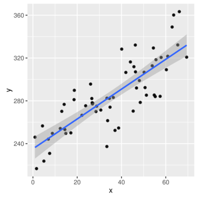
> library(ggplot2)
> ggplot(data.rcb, aes(y=y, x=x)) + geom_point() + geom_smooth(method='lm')

Example

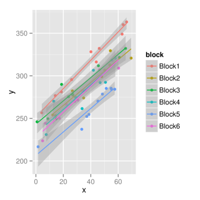
> library(ggplot2)
> ggplot(data.rcb, aes(y=y, x=x,color=block))+geom_point()+
+     geom_smooth(method='lm')

Example

Simple linear regression - wrong

> data.rcb.lm <- lm(y~x, data.rcb)

Generalized least squares - more correct

> library(nlme)
> data.rcb.gls <- gls(y~x, data.rcb, method='REML')

Example

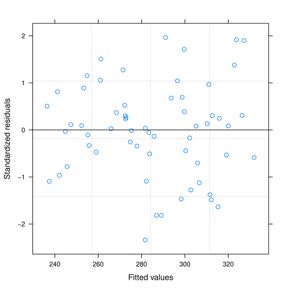
Model validation

> plot(data.rcb.gls)

Example

> plot(residuals(data.rcb.gls, type='normalized') ~
+      data.rcb$block)

- So what about ANCOVA

Example

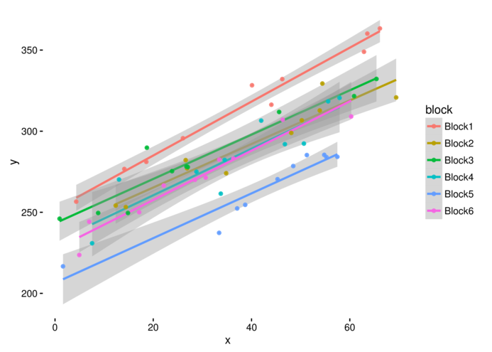
> library(ggplot2)
> ggplot(data.rcb, aes(y=y, x=x, color=block))+
+     geom_smooth(method="lm")+geom_point()+theme_classic()

Example

What if we add block as a predictor? (like ANCOVA)

> library(nlme)
> data.rcb.gls1 <- gls(y~x+block, data.rcb, method='REML')
> plot(data.rcb.gls)

Example

> plot(residuals(data.rcb.gls1, type='normalized') ~
+      data.rcb$block)

Example

Looks good, but for INDEPENDENCE
Can we deal with that with correlation structure?

\[ \text{Variance-covariance per Block:} \mathbf{V} = \begin{pmatrix} \sigma^2&\rho&\cdots&\rho\\ \rho&\sigma^2&\cdots&\vdots\\ \vdots&\cdots&\sigma^2&\vdots\\ \rho&\cdots&\cdots&\sigma^2\\ \end{pmatrix} \]

Example

Model in dependency structure

> library(nlme)
> data.rcb.gls2<-gls(y~x,data.rcb,
+                    correlation=corCompSymm(form=~1|block),
+                    method="REML")
> plot(residuals(data.rcb.gls2, type='normalized') ~
+      fitted(data.rcb.gls2))

Example

> plot(residuals(data.rcb.gls2, type='normalized') ~
+      data.rcb$block)

Example

> summary(data.rcb.gls2)

Generalized least squares fit by REML
  Model: y ~ x 
  Data: data.rcb 
       AIC      BIC   logLik
  458.9521 467.1938 -225.476

Correlation Structure: Compound symmetry
 Formula: ~1 | block 
 Parameter estimate(s):
      Rho 
0.8052553 

Coefficients:
               Value Std.Error  t-value p-value
(Intercept) 232.8193  7.823394 29.75937       0
x             1.4591  0.063789 22.87392       0

 Correlation: 
  (Intr)
x -0.292

Standardized residuals:
        Min          Q1         Med          Q3         Max 
-2.19174920 -0.59481155  0.05261311  0.59571239  1.83321624 

Residual standard error: 20.18017 
Degrees of freedom: 60 total; 58 residual

Linear mixed effects model

> data.rcb.lme <- lme(y~x, random=~1|block, data.rcb,
+                     method='REML')
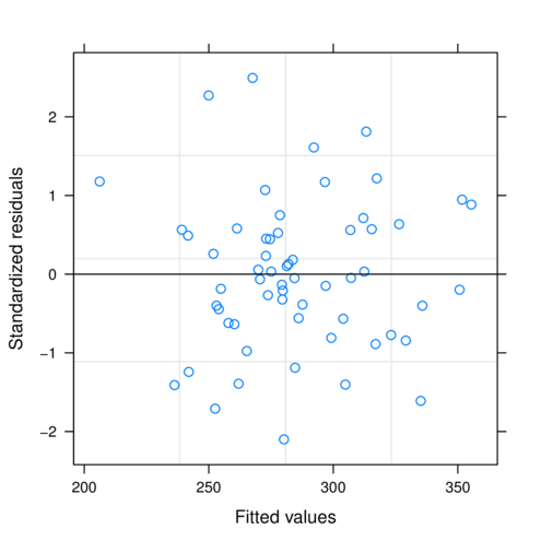
> plot(data.rcb.lme)

> plot(residuals(data.rcb.lme, type='normalized') ~ fitted(data.rcb.lme))

> plot(residuals(data.rcb.lme, type='normalized') ~ data.rcb$block)

Linear mixed effects model

> summary(data.rcb.lme)

Linear mixed-effects model fit by REML
 Data: data.rcb 
       AIC      BIC   logLik
  458.9521 467.1938 -225.476

Random effects:
 Formula: ~1 | block
        (Intercept) Residual
StdDev:    18.10888 8.905485

Fixed effects: y ~ x 
               Value Std.Error DF  t-value p-value
(Intercept) 232.8193  7.823393 53 29.75937       0
x             1.4591  0.063789 53 22.87392       0
 Correlation: 
  (Intr)
x -0.292

Standardized Within-Group Residuals:
        Min          Q1         Med          Q3         Max 
-2.09947262 -0.57994305 -0.04874031  0.56685096  2.49464217 

Number of Observations: 60
Number of Groups: 6

Linear mixed effects model

> anova(data.rcb.lme)

            numDF denDF   F-value p-value
(Intercept)     1    53 1452.2883  <.0001
x               1    53  523.2164  <.0001

> intervals(data.rcb.lme)

Approximate 95% confidence intervals

 Fixed effects:
                 lower       est.      upper
(Intercept) 217.127551 232.819291 248.511031
x             1.331156   1.459101   1.587045
attr(,"label")
[1] "Fixed effects:"

 Random Effects:
  Level: block 
                   lower     est.    upper
sd((Intercept)) 9.597555 18.10888 34.16822

 Within-group standard error:
    lower      est.     upper 
 7.361789  8.905485 10.772878

Linear mixed effects model

> vc<-as.numeric(as.matrix(VarCorr(data.rcb.lme))[,1])
> vc/sum(vc)

[1] 0.8052553 0.1947447

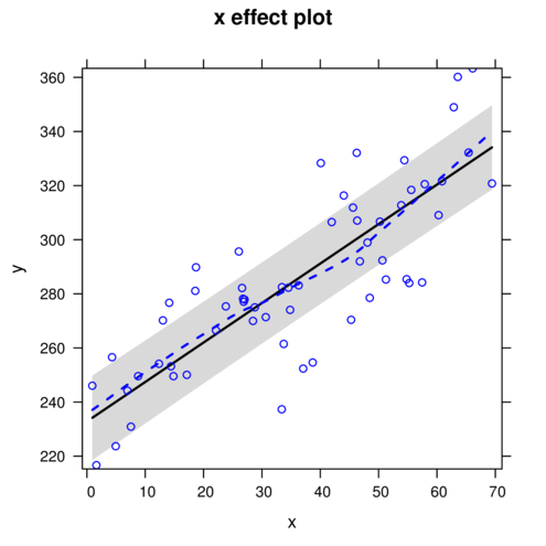
Linear mixed effects model

> library(effects)
> plot(allEffects(data.rcb.lme, partial.residuals=TRUE))

Linear mixed effects model

> predict(data.rcb.lme, newdata=data.frame(x=30:40),level=0)

 [1] 276.5923 278.0514 279.5105 280.9696 282.4287 283.8878 285.3469 286.8060 288.2651 289.7242
[11] 291.1833
attr(,"label")
[1] "Predicted values"

Linear mixed effects model

> predict(data.rcb.lme, newdata=data.frame(x=30:40,
+                           block='Block1'),level=1)

  Block1   Block1   Block1   Block1   Block1   Block1   Block1   Block1   Block1   Block1   Block1 
302.7422 304.2013 305.6604 307.1195 308.5786 310.0377 311.4968 312.9559 314.4150 315.8741 317.3332 
attr(,"label")
[1] "Predicted values"

Linear mixed effects model

Summary figure

Step 1. gather model coefficients

> coefs <- fixef(data.rcb.lme)
> coefs

(Intercept)           x 
 232.819291    1.459101

Linear mixed effects model

Summary figure

Step 2. generate prediction model matrix

> xs <- seq(min(data.rcb$x), max(data.rcb$x), l=100)
> Xmat <- model.matrix(~x, data.frame(x=xs))
> head(Xmat)

  (Intercept)         x
1           1 0.9373233
2           1 1.6292032
3           1 2.3210830
4           1 3.0129628
5           1 3.7048426
6           1 4.3967225

Linear mixed effects model

Summary figure

Step 3. calculate predicted y

> ys <- t(coefs %*% t(Xmat))
> head(ys)

Linear mixed effects model

Summary figure

Step 3. calculate confidence interval

> SE <- sqrt(diag(Xmat %*% vcov(data.rcb.lme) %*% t(Xmat)))
> CI <- 2*SE
> #OR
> CI <- qt(0.975,length(data.rcb$x)-2)*SE
> data.rcb.pred <- data.frame(x=xs, fit=ys, se=SE,
+      lower=ys-CI, upper=ys+CI)
> head(data.rcb.pred)

          x      fit       se    lower    upper
1 0.9373233 234.1869 7.806128 218.5613 249.8126
2 1.6292032 235.1965 7.793653 219.5958 250.7972
3 2.3210830 236.2060 7.781408 220.6298 251.7822
4 3.0129628 237.2155 7.769395 221.6634 252.7676
5 3.7048426 238.2250 7.757614 222.6965 253.7536
6 4.3967225 239.2346 7.746067 223.7291 254.7400

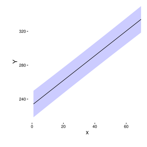
Linear mixed effects model

Summary figure

Step 4. plot it

> library(ggplot2)
> ggplot(data.rcb.pred, aes(y=fit, x=x)) +
+     geom_ribbon(aes(ymin=lower,ymax=upper),fill='blue',alpha=0.2)+
+     geom_line()+
+     scale_y_continuous('Y')+
+     theme_classic()+
+     theme(axis.title.x=element_text(size=rel(1.25), vjust=-2),
+           axis.title.y=element_text(size=rel(1.25), vjust=2),
+           plot.margin=unit(c(0.1,0.1,2,2),'lines'))
>  
> ## plot(fit~x, data=data.rcb.pred,type='n',axes=F, ann=F)
> ## points(y~x, data=data.rcb, pch=16, col='grey')
> ## with(data.rcb.pred, polygon(c(x,rev(x)), c(lower, rev(upper)),
> ##          col="#0000FF50",border=FALSE))
> ## lines(fit~x,data=data.rcb.pred)
> ## lines(lower~x,data=data.rcb.pred, lty=2)
> ## lines(upper~x,data=data.rcb.pred, lty=2)
> ## axis(1)
> ## mtext('X',1,line=3)
> ## axis(2,las=1)
> ## mtext('Y',2,line=3)
> ## box(bty='l')

Linear mixed effects model

Summary figure

Linear mixed effects model

Summary figure

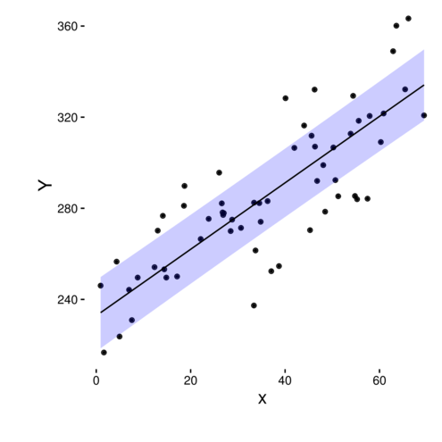
Step 4. plot it (with partial observed values)

> data.rcb$res <- predict(data.rcb.lme, level=1)+
+     residuals(data.rcb.lme)
> 
> library(ggplot2)
> ggplot(data.rcb.pred, aes(y=fit, x=x)) +
+     geom_point(data=data.rcb, aes(y=res))+
+     geom_ribbon(aes(ymin=lower,ymax=upper),fill='blue',alpha=0.2)+
+     geom_line()+
+     scale_y_continuous('Y')+
+     theme_classic()+
+     theme(axis.title.x=element_text(size=rel(1.25), vjust=-2),
+           axis.title.y=element_text(size=rel(1.25), vjust=2),
+           plot.margin=unit(c(0.1,0.1,2,2),'lines'))

Linear mixed effects model

Workshop 9.1: Mixed effects models

Murray Logan

10 Oct 2016

Non-independence - part 2

Linear models

Linear models

Hierarchical models

Hierarchical models

Hierarchical models

Nested design

Hierarchical models

Nested design

Hierarchical models

Nested design

Hierarchical models

Hierarchical models

Hierarchical models

Randomized complete block

Hierarchical models

Randomized complete block

Hierarchical models

Randomized complete block

Linear modelling assumptions

Non-independence

Hierarchical models

Example

Example

Example

Example

Example

Example

Example

Example

Example

Example

Example

Example

Example

Linear mixed effects model

Linear mixed effects model

Linear mixed effects model

Linear mixed effects model

Linear mixed effects model

Linear mixed effects model

Linear mixed effects model

Linear mixed effects model

Summary figure

Linear mixed effects model

Summary figure

Linear mixed effects model

Summary figure

Linear mixed effects model

Summary figure

Linear mixed effects model

Summary figure

Linear mixed effects model

Summary figure

Linear mixed effects model

Summary figure

Linear mixed effects model

Summary figure