Workshop 9.2a: Nested designs
Murray Logan
23 Nov 2016
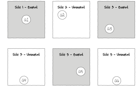
Nested design
Simple
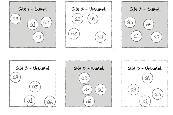
Nested
Nested design
> data.nest <- read.csv ('../data/data.nest.csv' )
> head (data.nest) y Region Sites Quads
1 32.25789 A S1 1
2 32.40160 A S1 2
3 37.20174 A S1 3
4 36.58866 A S1 4
5 35.45206 A S1 5
6 37.07744 A S1 6
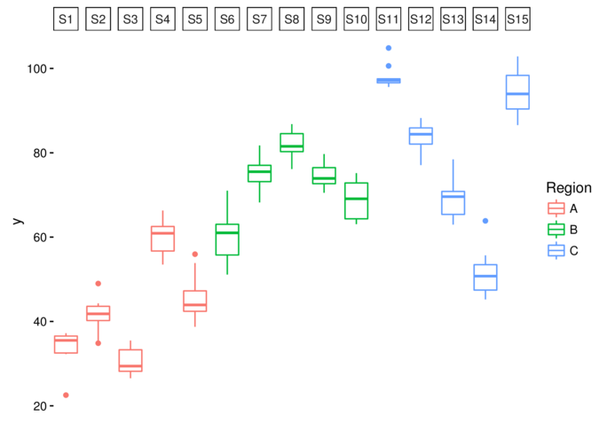
Nested design
> library (ggplot2)
> data.nest$Sites <- factor (data.nest$Sites, levels= paste0 ('S' ,1 :nSites))
> ggplot (data.nest, aes (y= y, x= 1 ,color= Region)) + geom_boxplot () +
+ facet_grid (.~Sites) +
+ scale_x_continuous ('' , breaks= NULL )+theme_classic ()
Nested design
> #Effects of treatment
> library (plyr)
> boxplot (y~Region, ddply (data.nest, ~Region+Sites,
+ numcolwise (mean, na.rm= T)))
Nested design
> #Site effects
> boxplot (y~Sites, ddply (data.nest, ~Region+Sites+Quads,
+ numcolwise (mean, na.rm= T)))
Nested design
\(y = \mu + \alpha + \beta(\alpha) + \epsilon\)
e.g.
\(abundance = base + burnt + quadrat(burnt)\)
Nested design
\(y = \mu + \alpha + \beta(\alpha) + \epsilon\\ y_{ijk} = \mu + \alpha_{i}{}Region_i + \beta_{j(i)}Sites_{j(i)} + \epsilon_{ijk}\)
\(\mu\) - base (mean of first Region)
\(\alpha\) - main fixed effect
\(\beta\) - sub-replicates (Sites: random effect)
> with (data.nest, table (Region,Sites)) Sites
Region S1 S2 S3 S4 S5 S6 S7 S8 S9 S10 S11 S12 S13 S14 S15
A 10 10 10 10 10 0 0 0 0 0 0 0 0 0 0
B 0 0 0 0 0 10 10 10 10 10 0 0 0 0 0
C 0 0 0 0 0 0 0 0 0 0 10 10 10 10 10> head (data.nest, 20 ) y Region Sites Quads
1 32.25789 A S1 1
2 32.40160 A S1 2
3 37.20174 A S1 3
4 36.58866 A S1 4
5 35.45206 A S1 5
6 37.07744 A S1 6
7 36.39324 A S1 7
8 32.85538 A S1 8
9 22.53580 A S1 9
10 35.58168 A S1 10
11 41.92308 A S2 11
12 41.42474 A S2 12
13 34.84996 A S2 13
14 39.81297 A S2 14
15 44.29343 A S2 15
16 48.99712 A S2 16
17 41.68978 A S2 17
18 44.14208 A S2 18
19 41.93469 A S2 19
20 35.31842 A S2 20
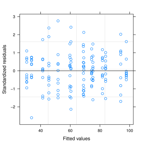
Nested design
\(y = \mu + \alpha + \beta(\alpha) + \epsilon\\ y_{ijk} = \mu + \alpha_{i}{}Region_i + \beta_{j(i)}Sites_{j(i)} + \epsilon_{ijk}\)
> library (nlme)
> data.nest.lme <- lme (y~Region, random= ~1 |Sites, data.nest)
> plot (data.nest.lme)
Nested design
> plot (data.nest$Region, residuals (data.nest.lme,
+ type= 'normalized' ))
Nested design
> summary (data.nest.lme)Linear mixed-effects model fit by REML
Data: data.nest
AIC BIC logLik
927.7266 942.6788 -458.8633
Random effects:
Formula: ~1 | Sites
(Intercept) Residual
StdDev: 13.6582 4.372252
Fixed effects: y ~ Region
Value Std.Error DF t-value p-value
(Intercept) 42.27936 6.139350 135 6.886618 0.0000
RegionB 29.84692 8.682352 12 3.437654 0.0049
RegionC 37.02026 8.682352 12 4.263851 0.0011
Correlation:
(Intr) ReginB
RegionB -0.707
RegionC -0.707 0.500
Standardized Within-Group Residuals:
Min Q1 Med Q3 Max
-2.603787242 -0.572951701 0.004953998 0.620914933 2.765601716
Number of Observations: 150
Number of Groups: 15
Nested design
> VarCorr (data.nest.lme)Sites = pdLogChol(1)
Variance StdDev
(Intercept) 186.54644 13.658200
Residual 19.11659 4.372252> anova (data.nest.lme) numDF denDF F-value p-value
(Intercept) 1 135 331.8308 <.0001
Region 2 12 10.2268 0.0026
Nested design
> library (multcomp)
> summary (glht (data.nest.lme, linfct= mcp (Region= "Tukey" )))
     Simultaneous Tests for General Linear Hypotheses

Multiple Comparisons of Means: Tukey Contrasts


Fit: lme.formula(fixed = y ~ Region, data = data.nest, random = ~1 |
    Sites)

Linear Hypotheses:
           Estimate Std. Error z value Pr(>|z|)
B - A == 0   29.847      8.682   3.438  0.00172 **
C - A == 0   37.020      8.682   4.264  < 0.001 ***
C - B == 0    7.173      8.682   0.826  0.68674
---
Signif. codes:  0 '***' 0.001 '**' 0.01 '*' 0.05 '.' 0.1 ' ' 1
(Adjusted p values reported -- single-step method)
Nested design
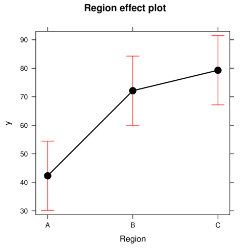
> library (effects)
> plot (allEffects (data.nest.lme))
Linear mixed effects model
Step 1. gather model coefficients and model matrix
> coefs <- fixef (data.nest.lme)
> coefs(Intercept) RegionB RegionC
42.27936 29.84692 37.02026 > xs <- levels (data.nest$Region)
> Xmat <- model.matrix (~Region, data.frame (Region= xs))
> head (Xmat) (Intercept) RegionB RegionC
1 1 0 0
2 1 1 0
3 1 0 1
Linear mixed effects model
Step 3. calculate predicted y and CI
> ys <- t (coefs %*% t (Xmat))
> head (ys) [,1]
1 42.27936
2 72.12628
3 79.29961> SE <- sqrt (diag (Xmat %*% vcov (data.nest.lme) %*% t (Xmat)))
> CI <- 2 *SE
> #OR
> CI <- qt (0.975 ,length (data.nest$y)-2 )*SE
> data.nest.pred <- data.frame (Region= xs, fit= ys, se= SE,
+ lower= ys-CI, upper= ys+CI)
> head (data.nest.pred) Region fit se lower upper
1 A 42.27936 6.13935 30.14725 54.41147
2 B 72.12628 6.13935 59.99417 84.25839
3 C 79.29961 6.13935 67.16751 91.43172
Linear mixed effects model
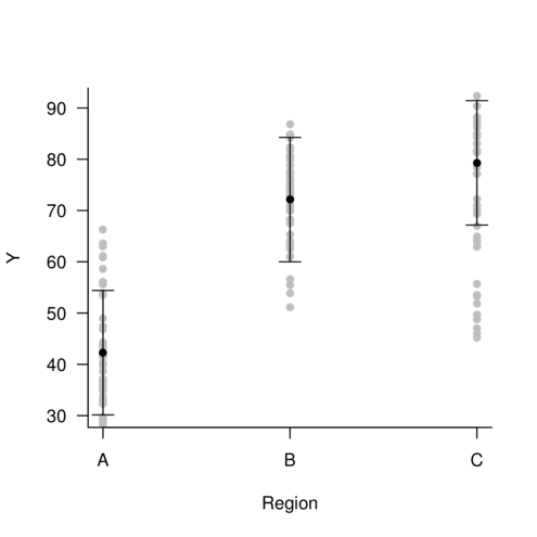
Step 4. plot it
> with (data.nest.pred,plot.default (Region, fit,type= 'n' ,axes= F, ann= F,ylim= range (c (data.nest.pred$lower, data.nest.pred$upper))))
> points (y~Region, data= data.nest, pch= 16 , col= 'grey' )
> points (fit~Region, data= data.nest.pred, pch= 16 )
> with (data.nest.pred, arrows (as.numeric (Region),lower,as.numeric (Region),upper, length= 0.1 , angle= 90 , code= 3 ))
> axis (1 , at= 1 :3 , labels= levels (data.nest$Region))
> mtext ('Region' ,1 ,line= 3 )
> axis (2 ,las= 1 )
> mtext ('Y' ,2 ,line= 3 )
> box (bty= 'l' )
Linear mixed effects model
Linear mixed effects model
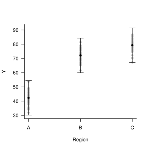
Step 4. plot it
> data.nest$res <- predict (data.nest.lme, level= 0 )-
+ residuals (data.nest.lme)
> with (data.nest.pred,plot.default (Region, fit,type= 'n' ,axes= F, ann= F,ylim= range (c (data.nest.pred$lower, data.nest.pred$upper))))
> points (res~Region, data= data.nest, pch= 16 , col= 'grey' )
> points (fit~Region, data= data.nest.pred, pch= 16 )
> with (data.nest.pred, arrows (as.numeric (Region),lower,as.numeric (Region),upper, length= 0.1 , angle= 90 , code= 3 ))
> axis (1 , at= 1 :3 , labels= levels (data.nest$Region))
> mtext ('Region' ,1 ,line= 3 )
> axis (2 ,las= 1 )
> mtext ('Y' ,2 ,line= 3 )
> box (bty= 'l' )
Linear mixed effects model
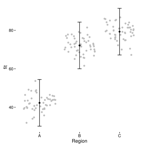
Linear mixed effects model
> library (ggplot2)
> data.nest$res <- predict (data.nest.lme, level= 0 )-
+ residuals (data.nest.lme)
>
> ggplot (data.nest.pred, aes (y= fit, x= Region))+
+ geom_point (data= data.nest, aes (y= res), col= 'grey' ,position = position_jitter (height= 0 ))+
+ geom_errorbar (aes (ymin= lower, ymax= upper), width= 0.1 )+
+ geom_point ()+
+ theme_classic ()+
+ theme (axis.title.y= element_text (vjust= 2 ),
+ axis.title.x= element_text (vjust= -1 ))
Linear mixed effects model
Worked Examples
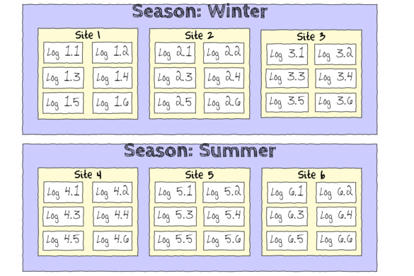
Format of curdies.csv data files
SEASON
SITE
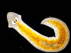
DUGESIA
S4DUGESIA
WINTER
1
0.648
0.897
..
..
..
..
WINTER
2
1.016
1.004
..
..
..
..
WINTER
3
0.689
0.991
..
..
..
..
SUMMER
4
0
0
..
..
..
..
Each row represents a different stone
SEASON
Season in which flatworms were counted - fixed factor
SITE
Site from where flatworms were counted - nested within SEASON (random factor)
DUGESIA
Number of flatworms counted on a particular stone
S4DUGESIA
4th root transformation of DUGESIA variable
Worked Examples