Tutorial 11.2b - Goodness of fit tests
11 Mar 2015
library(R2jags)
library(plyr)
Scenario and Data
Goodness of fit tests are concerned with comparing the observed frequencies with those expected on the basis of a specific null hypothesis. So lets now fabricate a motivating scenario and some data.
We will create a scenario that involves items classified into one of three groups (A, B and C). The number of items in each classification group are then tallied up. Out of a total of 47 items, 15 where of type A, 9 where of type B and 23 where of type C. We could evaluate a parity (a 1:1:1 ratio from these data. In a frequentist context, this might involve testing a null hypothesis that the observed data could have come from a population with a 1:1 item ratio. In this case the probability would be the probability of obtaining the observed ratio of frequencies when the null hypothesis is true.
In a Bayesian context, there are numerous ways that we could tackle these data. We would be evaluating the evidence for the null hypothesis (1:1:1 item ratio) given the observed by estimating the degree of freedom from a chi-square distribution. Alternatively, we could estimate the value of the three population fractions which are expected to be 1/3, 1/3, 1/3 when 1:1:1. We will explore this option first and then explore the chi-square approach second.
To extend the example, lets also explore a 1:1:2 ratio.
We start by generating the observed data:
#the observed frequences of A and B
obs <- c(15,9,23)
obs
[1] 15 9 23
Estimating population fractions - binomial distribution
The binomial distribution represents the distribution of possible densities (probabilities) for the number of successes $p$ out of a total of $n$ independent trials. In this case, it can be used to model the number of items of each group (A, B and C) out of a total of 47 items. The prior distribution for $p_i$ would be a beta distribution (values range from 0 to 1) with shape parameters $a$ and $b$ the hyperpriors of which follow vague (flat, imprecise) gamma distributions. \begin{align*} obs_i &\sim Bin(p_i,n_i)\\ p_i &\sim B(a_i,b_i)\\ a &\sim gamma(1, 0.01)\\ b &\sim gamma(1, 0.01) \end{align*}
Exploratory data analysis and initial assumption checking
The data should logically follow a binomial distribution (since the observations are counts of positive events out of a total).
Model fitting or statistical analysis
Define the model
We now translate the likelihood model into BUGS/JAGS code and store the code in an external file.
modelString="
model {
  #Likelihood
 for (i in 1:nGroups) {
   obs[i] ~ dbin(p[i],n[i])
   p[i] ~ dbeta(a[i],b[i])
   a[i] ~ dgamma(1,0.01)
   b[i] ~ dgamma(1,0.01)
 }
 }
"
## write the model to a text file (I suggest you alter the path to somewhere more relevant
## to your system!)
writeLines(modelString,con="../downloads/BUGSscripts/tut11.2bQ1.1.txt")
- The likelihood model indicates that the observed counts are modeled by a binomial distribution with a probability of $p$ (fraction) from $n$ trials (items).
- The prior on each $p$ is defined as a beta distribution with shape parameters $a$ and $b$
- The hyperpriors for each $a$ and $b$ are drawn from imprecise (vague, flat) gamma distributions.
Define the data list
As input, JAGS will need to be supplied with:
- the observed data ($obs$)
- the total number of observed items ($n$)
- the number of classification groups ($nGroups$)
# The observed item frequencies
obs <- c(15, 9, 23)
data.list <- list(obs = obs, n = c(47, 47, 47), nGroups = 3)
data.list
$obs
[1] 15  9 23

$n
[1] 47 47 47

$nGroups
[1] 3
Define the MCMC chain parameters
Next we should define the behavioural parameters of the MCMC sampling chains. Include the following:
- the nodes (estimated parameters) to monitor (return samples for)
- the number of MCMC chains (3)
- the number of burnin steps (1000)
- the thinning factor (10)
- the number of MCMC iterations - determined by the number of samples to save, the rate of thinning and the number of chains
params <- c("p")
nChains = 3
burnInSteps = 1000
thinSteps = 10
numSavedSteps = 5000
nIter = ceiling((numSavedSteps * thinSteps)/nChains)
Fit the model
Now run the JAGS code via the R2jags interface. Note that the first time jags is run after the R2jags package is loaded, it is often necessary to run any kind of randomization function just to initiate the .Random.seed variable.
# Run any random function just to get .Random.seed started
runif(1)
[1] 0.2553
# Fit the model for the 1:1:1 ratio
data.r2jags <- jags(data = data.list, inits = NULL, parameters.to.save = params, model.file = "../downloads/BUGSscripts/tut11.2bQ1.1.txt",
    n.chains = 3, n.iter = nIter, n.burnin = burnInSteps, n.thin = thinSteps)
Compiling model graph
   Resolving undeclared variables
   Allocating nodes
   Graph Size: 18

Initializing model
print(data.r2jags)
Inference for Bugs model at "../downloads/BUGSscripts/tut11.2bQ1.1.txt", fit using jags,
 3 chains, each with 16667 iterations (first 1000 discarded), n.thin = 10
 n.sims = 4701 iterations saved
         mu.vect sd.vect   2.5%    25%    50%    75%  97.5%  Rhat n.eff
p[1]       0.326   0.067  0.204  0.279  0.323  0.369  0.464 1.001  4700
p[2]       0.203   0.057  0.104  0.162  0.198  0.239  0.327 1.001  4700
p[3]       0.490   0.072  0.354  0.442  0.490  0.539  0.632 1.001  4700
deviance  15.277   2.411 12.537 13.512 14.649 16.363 21.836 1.001  2700

For each parameter, n.eff is a crude measure of effective sample size,
and Rhat is the potential scale reduction factor (at convergence, Rhat=1).

DIC info (using the rule, pD = var(deviance)/2)
pD = 2.9 and DIC = 18.2
DIC is an estimate of expected predictive error (lower deviance is better).
Conclusions: Initially, we should focus our attention on the Rhat and n.eff columns. These are the scale reduction and number of effective samples respectively and they provide an indication of the degree of mixing or coverage of the samples. Ideally, the n.eff values should be approximately equal to the number of saved samples (in this case 4701), and the Rhat values should be approximately 1 (complete convergence).
Whilst the actual values are likely to differ substantially from run to run (due to the stochastic nature of the way the chains traverse the posterior distribution), on this occasion, the n.eff of the first two probability parameters (p[1] and p[2]) are substantially lower than 4700. Hence, the samples of these parameters may not accurately reflect the posterior distribution. We might consider altering one or more of the chain behavioural paramters (such as the thinning rate), alter the model definition (or priors) itself.
Model evaluation
Prior to exploring the model parameters, it is necessary to first evaluate whether the MCMC samples are likely to be representative of a stationary posterior distribution. Specifically, we should explore:
- whether the MCMC chains have converged - Trace plots
- whether the MCMC chains have yielded well mixed (not autocorrelated samples) - Raftery and autocorrelation diagnostics
- whether the MCMC samples are independent of the initial starting configuration (adequate burnin) - Trace plots
- What sort of point estimates (mean, median and mode) are appropriate for the parameters - Density plots
- Trace and density plots
For the Goodness of fit test, it is only the distribution of the $p$'s that we are interested inAlternatively, you could request traces and density plots for all monitored nodes (parameters)library(plyr) library(coda) preds <- c("p[1]", "p[2]", "p[3]") plot(as.mcmc.list(alply(data.r2jags$BUGSoutput$sims.array[, , preds], 2, function(x) { as.mcmc(x) })))
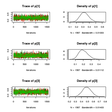 Conclusions: the trace plots show what appears to be "random noise" about the parameter value. There is no real suggestion of a step or dramatic change in the trend direction along the length of the sampling chain. The samples seem relatively stable. Thus it would seem that the chains are well mixed and have converged. The density plots (for $p$) are vaguely symmetrical. This suggests that either the mean or the median are good point estimates for these parameters.
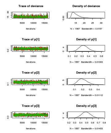
plot(as.mcmc(data.r2jags))
- Autocorrelation diagnostic
preds <- c("p[1]", "p[2]", "p[3]")
autocorr.diag(as.mcmc.list(alply(data.r2jags$BUGSoutput$sims.array[, , preds], 2, function(x) {
    as.mcmc(x)
})))
            p[1]      p[2]      p[3]
Lag 0   1.000000  1.000000  1.000000
Lag 1   0.117459  0.149863  0.125074
Lag 5  -0.004215 -0.023109  0.002661
Lag 10 -0.027707  0.015376  0.001922
Lag 50 -0.017148  0.008875 -0.009350
Conclusions: At the specified lag (thinning rate of 10), there is some evidence of autocorrelation. The diagnostics suggest that a lag of 50 (thinning rate of 50) would yield samples that are better mixed. So we should really refit the model with a higher thinning rate.autocorr.diag(as.mcmc(data.r2jags))
         deviance      p[1]      p[2]      p[3]
Lag 0    1.000000  1.000000  1.000000  1.000000
Lag 10   0.038632  0.117459  0.149863  0.125074
Lag 50  -0.020213 -0.004215 -0.023109  0.002661
Lag 100  0.025016 -0.027707  0.015376  0.001922
Lag 500 -0.009744 -0.017148  0.008875 -0.009350
- Raftery diagnostic
Conclusions: Minimum required number of MCMC samples to ensure that sufficient samples had been collected to achieve good accuracy is 3746. We had 5000 per chain ($5000\times3=15000$).
raftery.diag(as.mcmc(data.r2jags))
[[1]]

Quantile (q) = 0.025
Accuracy (r) = +/- 0.005
Probability (s) = 0.95

You need a sample size of at least 3746 with these values of q, r and s

[[2]]

Quantile (q) = 0.025
Accuracy (r) = +/- 0.005
Probability (s) = 0.95

You need a sample size of at least 3746 with these values of q, r and s

[[3]]

Quantile (q) = 0.025
Accuracy (r) = +/- 0.005
Probability (s) = 0.95

You need a sample size of at least 3746 with these values of q, r and s
params <- c("p")
nChains = 3
burnInSteps = 1000
thinSteps = 50
numSavedSteps = 5000
nIter = ceiling((numSavedSteps * thinSteps)/nChains)
data.r2jags <- jags(data = data.list, inits = NULL, parameters.to.save = params, model.file = "../downloads/BUGSscripts/tut11.2bQ1.1.txt",
    n.chains = 3, n.iter = nIter, n.burnin = burnInSteps, n.thin = thinSteps)
Compiling model graph
   Resolving undeclared variables
   Allocating nodes
   Graph Size: 18

Initializing model
print(data.r2jags)
Inference for Bugs model at "../downloads/BUGSscripts/tut11.2bQ1.1.txt", fit using jags,
 3 chains, each with 83334 iterations (first 1000 discarded), n.thin = 50
 n.sims = 4941 iterations saved
         mu.vect sd.vect   2.5%    25%    50%    75%  97.5%  Rhat n.eff
p[1]       0.327   0.066  0.205  0.279  0.324  0.371  0.459 1.001  4600
p[2]       0.204   0.057  0.103  0.163  0.200  0.239  0.326 1.001  4900
p[3]       0.489   0.071  0.348  0.442  0.488  0.536  0.630 1.001  4900
deviance  15.232   2.379 12.551 13.523 14.612 16.262 21.286 1.002  2000

For each parameter, n.eff is a crude measure of effective sample size,
and Rhat is the potential scale reduction factor (at convergence, Rhat=1).

DIC info (using the rule, pD = var(deviance)/2)
pD = 2.8 and DIC = 18.1
DIC is an estimate of expected predictive error (lower deviance is better).
Conclusions: Rhat and n.eff are now much better for the probability parameters. The estimated fractions for A, B and C are:
- A: 0.327 (0.207, 0.466)
- B: 0.200 (0.104, 0.323)
- C: 0.491 (0.355, 0.625)
Chi-square
An appropriate test statistic for comparing an observed ($o$) frequency ratio to an expected ($e$) frequency ratio is the chi-square $\chi^2$ statistic. $$\chi^2=\sum\frac{(o-e)^2}{e}$$ In effect, the chi-square statistic (which incorporates the variability in the data in to measure of the difference between observed and expected) becomes the input for the likelihood model. Whilst we could simply pass JAGS the chi-square statistic, by parsing the observed and expected values and having the chi-square value calculated within JAGS data, the resulting JAGS code is more complete and able to accommodate other scenarios.
So if, $chisq$ is the chi-square statistic and $k$ is the degrees of freedom (and thus expected value of the $\chi^2$ distribution), then the likelihood model is:
\begin{align*} chisq &\sim \chi^2(k)\\ k &\sim U(0.01, 100) \end{align*}Exploratory data analysis and initial assumption checking
- All of the observations are classified independently - this must be addressed at the design and collection stages
- No more than 20% of the expected values should be less than 5. Since the location and spread of the expected value of a $\chi^2$ distribution are the same parameter ($\lambda$), and that the $\chi^2$ distribution is bounded by a lower limit of zero, distributions with expected values less than 5 have an asymmetrical shape and are thus unreliable (for calculating probabilities).
So lets calculate the expected frequencies as a means to evaluate this assumption. The expected values are calculated as: $$e = total~counts \times expected~fraction$$
| 1:1:1 ratio | 1:1:2 ratio | |
|---|---|---|
| Expected fractions | A=1/3=0.33, B=1/3=0.33, C=1/3=0.33 | A=1/3=0.25, B=1/4=0.25, C=2/4=0.5 |
| Expected frequencies | $e_A=(15+9+23)\times 1/3=15.67$ $e_B=(15+9+23)\times 1/3=15.67$ $e_C=(15+9+23)\times 1/3=15.67$ | $e_A=(15+9+23)\times 1/4=11.75$ $e_B=(15+9+23)\times 1/4=11.75$ $e_C=(15+9+23)\times 2/4=23.5$ |
It is clear that in neither case are any of the expected frequencies less than 5. Therefore, we would conclude that probabilities derived from the $\chi^2$ distribution are likely to be reliable.
Model fitting or statistical analysis
Define the model
We now translate the likelihood model into BUGS/JAGS code and store the code in an external file.
modelString="
data {
for (i in 1:n){
     resid[i] <- pow(obs[i]-exp[i],2)/exp[i]
   }
   chisq <- sum(resid)
}
model {
  #Likelihood
  chisq  ~ dchisqr(k)
  #Priors
  k ~ dunif(0.01,100)
 }
"
## write the model to a text file (I suggest you alter the path to somewhere more relevant
## to your system!)
writeLines(modelString,con="../downloads/BUGSscripts/tut11.2bQ2.1.txt")
- First of all, the standardized residuals and chi-square statistic are calculated according to the formula listed above.
- The likelihood model indicates that the chi-squared statistic can be modeled by a $\chi^2$ distribution with a centrality parameter of $k$.
- The prior on $k$ is defined as a uniform (thus vague) flat prior whose values could range from 0.01 to 100 (all with equal probability).
Define the data list
As input, JAGS will need to be supplied with:
- the observed data ($obs$)
- the expected frequencies ($exp$) (based on the hypothesis)
- the total number of observed items ($n$)
# The observed item frequencies
obs <- c(15, 9, 23)
# The expected item frequencies (for a 1:1:1 ratio)
exp <- rep(sum(obs) * 1/3, 3)
data.list <- list(obs = obs, exp = exp, n = 3)
data.list
$obs
[1] 15  9 23

$exp
[1] 15.67 15.67 15.67

$n
[1] 3
# The expected item frequencies (for a 1:1:2 ratio)
exp <- sum(obs) * c(1/4, 1/4, 2/4)
data.list1 <- list(obs = obs, exp = exp, n = 3)
data.list1
$obs
[1] 15  9 23

$exp
[1] 11.75 11.75 23.50

$n
[1] 3
Define the MCMC chain parameters
Next we should define the behavioural parameters of the MCMC sampling chains. Include the following:
- the nodes (estimated parameters) to monitor (return samples for)
- the number of MCMC chains (3)
- the number of burnin steps (1000)
- the thinning factor (10)
- the number of MCMC iterations - determined by the number of samples to save, the rate of thinning and the number of chains
params <- c("chisq", "resid", "k")
nChains = 3
burnInSteps = 1000
thinSteps = 10
numSavedSteps = 5000
nIter = ceiling((numSavedSteps * thinSteps)/nChains)
Fit the model
Now run the JAGS code via the R2jags interface. Note that the first time jags is run after the R2jags package is loaded, it is often necessary to run any kind of randomization function just to initiate the .Random.seed variable.
# Run any random function just to get .Random.seed started
runif(1)
[1] 0.5516
# Fit the model for the 1:1:1 ratio
data.r2jags <- jags(data = data.list, inits = NULL, parameters.to.save = params, model.file = "../downloads/BUGSscripts/tut11.2bQ2.1.txt",
    n.chains = 3, n.iter = nIter, n.burnin = burnInSteps, n.thin = thinSteps)
Compiling data graph
   Resolving undeclared variables
   Allocating nodes
   Initializing
   Reading data back into data table
Compiling model graph
   Resolving undeclared variables
   Allocating nodes
   Graph Size: 14

Initializing model
# Fit the model for the 1:1:2 ratio
data.r2jags1 <- jags(data = data.list1, inits = NULL, parameters.to.save = params, model.file = "../downloads/BUGSscripts/tut11.2bQ2.1.txt",
    n.chains = 3, n.iter = nIter, n.burnin = burnInSteps, n.thin = thinSteps)
Compiling data graph
   Resolving undeclared variables
   Allocating nodes
   Initializing
   Reading data back into data table
Compiling model graph
   Resolving undeclared variables
   Allocating nodes
   Graph Size: 14

Initializing model
Model evaluation
Prior to exploring the model parameters, it is necessary to first evaluate whether the MCMC samples are likely to be representative of a stationary posterior distribution. Specifically, we should explore:
- whether the MCMC chains have converged - Trace plots
- whether the MCMC chains have yielded well mixed (not autocorrelated samples) - Raftery and autocorrelation diagnostics
- whether the MCMC samples are independent of the initial starting configuration (adequate burnin) - Trace plots
- What sort of point estimates (mean, median and mode) are appropriate for the parameters - Density plots
- Trace and density plots
For the Goodness of fit test, it is only the distribution of $k$ (degrees of freedom) that we are interested inAlternatively, you could request traces and density plots for all monitored nodes (parameters)library(plyr) library(coda) preds <- c("k") plot(as.mcmc.list(alply(data.r2jags$BUGSoutput$sims.array[, , preds], 2, function(x) { as.mcmc(x) })))
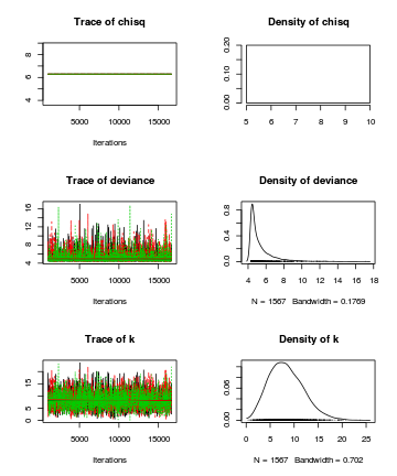
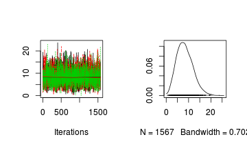 Conclusions: the trace plots show what appears to be "random noise" about the parameter value. There is no real suggestion of a step or dramatic change in the trend direction along the length of the sampling chain. The samples seem relatively stable. Thus it would seem that the chains are well mixed and have converged. The density plot (for $k$) is not symmetrical. This suggests that the mean is not a good point estimate for this parameter - the median would be better.
plot(as.mcmc(data.r2jags))

- Autocorrelation diagnostic
preds <- c("k")
autocorr.diag(as.mcmc.list(alply(data.r2jags$BUGSoutput$sims.array[, , preds], 2, function(x) {
    as.mcmc(x)
})))
             [,1]
Lag 0   1.0000000
Lag 1  -0.0008690
Lag 5  -0.0249016
Lag 10  0.0028189
Lag 50 -0.0002074
Conclusions: There is no evidence of autocorrelation at the specified lag (thinning rate of 10), so again, we would conclude that there is no evidence that the chain samples are not well mixed.autocorr.diag(as.mcmc(data.r2jags))
        chisq   deviance          k resid[1] resid[2] resid[3]
Lag 0     NaN  1.0000000  1.0000000      NaN      NaN      NaN
Lag 10    NaN -0.0112525 -0.0008690      NaN      NaN      NaN
Lag 50    NaN -0.0180426 -0.0249016      NaN      NaN      NaN
Lag 100   NaN  0.0002117  0.0028189      NaN      NaN      NaN
Lag 500   NaN -0.0224411 -0.0002074      NaN      NaN      NaN
- Raftery diagnostic
Conclusions: Minimum required number of MCMC samples to ensure that sufficient samples had been collected to achieve good accuracy is 3746. We had 5000 per chain ($5000\times3=15000$).
raftery.diag(as.mcmc(data.r2jags))
[[1]]

Quantile (q) = 0.025
Accuracy (r) = +/- 0.005
Probability (s) = 0.95

You need a sample size of at least 3746 with these values of q, r and s

[[2]]

Quantile (q) = 0.025
Accuracy (r) = +/- 0.005
Probability (s) = 0.95

You need a sample size of at least 3746 with these values of q, r and s

[[3]]

Quantile (q) = 0.025
Accuracy (r) = +/- 0.005
Probability (s) = 0.95

You need a sample size of at least 3746 with these values of q, r and s
Exploring the model parameters, test hypotheses
If there was any evidence that the assumptions had been violated, the model was not an appropriate fit or the MCMC chains had not converged or mixed thoroughly, then we would need to reconsider the model and start the process again. In this case, there is no evidence that the test will be unreliable so we can proceed to explore the test statistics.
print(data.r2jags)
Inference for Bugs model at "../downloads/BUGSscripts/tut11.2bQ2.1.txt", fit using jags,
 3 chains, each with 16667 iterations (first 1000 discarded), n.thin = 10
 n.sims = 4701 iterations saved
         mu.vect sd.vect  2.5%   25%   50%    75%  97.5%  Rhat n.eff
chisq      6.298   0.000 6.298 6.298 6.298  6.298  6.298 1.000     1
k          8.354   3.593 2.309 5.731 8.047 10.693 16.281 1.001  4700
resid[1]   0.028   0.000 0.028 0.028 0.028  0.028  0.028 1.000     1
resid[2]   2.837   0.000 2.837 2.837 2.837  2.837  2.837 1.000     1
resid[3]   3.433   0.000 3.433 3.433 3.433  3.433  3.433 1.000     1
deviance   5.339   1.378 4.346 4.448 4.820  5.662  9.239 1.002  2500

For each parameter, n.eff is a crude measure of effective sample size,
and Rhat is the potential scale reduction factor (at convergence, Rhat=1).

DIC info (using the rule, pD = var(deviance)/2)
pD = 0.9 and DIC = 6.3
DIC is an estimate of expected predictive error (lower deviance is better).
print(data.r2jags1)
Inference for Bugs model at "../downloads/BUGSscripts/tut11.2bQ2.1.txt", fit using jags,
 3 chains, each with 16667 iterations (first 1000 discarded), n.thin = 10
 n.sims = 4701 iterations saved
         mu.vect sd.vect  2.5%   25%   50%   75% 97.5%  Rhat n.eff
chisq      1.553   0.000 1.553 1.553 1.553 1.553 1.553 1.000     1
k          3.371   1.895 0.636 1.946 3.071 4.485 7.722 1.001  4700
resid[1]   0.899   0.000 0.899 0.899 0.899 0.899 0.899 1.000     1
resid[2]   0.644   0.000 0.644 0.644 0.644 0.644 0.644 1.000     1
resid[3]   0.011   0.000 0.011 0.011 0.011 0.011 0.011 1.000     1
deviance   3.836   1.398 2.870 2.964 3.321 4.133 7.729 1.002  2200

For each parameter, n.eff is a crude measure of effective sample size,
and Rhat is the potential scale reduction factor (at convergence, Rhat=1).

DIC info (using the rule, pD = var(deviance)/2)
pD = 1.0 and DIC = 4.8
DIC is an estimate of expected predictive error (lower deviance is better).
Further explorations of the trends
There are a number of avenues we could take in order to explore the data and models further. One thing we could do is calculate the probability that $k$ is greater than 2 (the expected value) for each hypothesis. This can be done either by modifying the BUGS/JAGS code to include a derivative that uses the step function, or we can derive it within R from the $k$ samples. Lets explore the latter.
k <- data.r2jags$BUGSoutput$sims.matrix[, "k"]
pr <- sum(k > 2)/length(k)
pr
[1] 0.984
k <- data.r2jags1$BUGSoutput$sims.matrix[, "k"]
pr1 <- sum(k > 2)/length(k)
pr1
[1] 0.7354
We could also compare the two alternative hypotheses. The 1:1:2 hypothesis has lower DIC and is therefore considered a better fit (4.7 vs 6.4). This is a difference in DIC of around 1.7 units. So the data have higher support for a 1:1:2 population ratio than a 1:1:1 ratio.
Worked Examples
Basic χ2 references
- Logan (2010) - Chpt 16-17
- Quinn & Keough (2002) - Chpt 13-14
Goodness of fit test
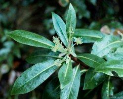
A fictitious plant ecologist sampled 90 shrubs of a dioecious plant in a forest, and each plant was classified as being either male or female. The ecologist was interested in the sex ratio and whether it differed from 50:50. The observed counts and the predicted (expected) counts based on a theoretical 50:50 sex ratio follow.
| Format of fictitious plant sex ratios - note, not a file | |||||||||||||
|---|---|---|---|---|---|---|---|---|---|---|---|---|---|
Expected and Observed data (50:50 sex ratio).
|
 |
Note, it is not necessary to open or create a data file for this question.
- As the fictitious researcher was interested in exploring sex parity (1:1 frequency ratio) in the dioecious plant,
the $\chi^2$ statistic would seem appropriate. Recall that the $\chi^2$ statistic is defined as:
$$\chi^2=\sum\frac{(o-e)^2}{e}$$
In effect, the chi-square statistic (which incorporates the variability in the data in to measure of the difference between observed and expected)
becomes the input for the likelihood model. Whilst we could simply pass JAGS the chi-square statistic, by
parsing the observed and expected values and having the chi-square value calculated within JAGS data,
the resulting JAGS code is more complete and able to accommodate other scenarios.
So if, $chisq$ is the chi-square statistic and $k$ is the degrees of freedom (and thus expected value of the $\chi^2$ distribution), then the likelihood model is:
\begin{align*} chisq &\sim \chi^2(k)\\ k &\sim U(0.01, 100) \end{align*} Translate this into JAGS code.Show codemodelString=" data { for (i in 1:n){ resid[i] <- pow(obs[i]-exp[i],2)/exp[i] } chisq <- sum(resid) } model { #Likelihood chisq ~ dchisqr(k) k ~ dunif(0.01,100) } " ## write the model to a text file (I suggest you alter the path to somewhere more relevant ## to your system!) writeLines(modelString,con="../downloads/BUGSscripts/ws11.2bQ1.1.txt")
-
We can now generate the observed and expected data as a list (as is necessary for JAGS).
When exploring parity, we are "expecting" the number of Females and Males to be very similar.
So from 90 individuals we expect 50% (0.5) to be Female and 50% to be Male.
To supply the JAGS code created in the step above, we require the observed counts, expected counts
and the number of classification levels ($=2$, Females and Males).
Show code
# The observed Female and Male plant frequencies
obs <- c(40, 50)
# The expected Female and Make plant frequencies
exp <- rep(sum(obs) * 0.5, 2)
plant.list <- list(obs = c(40, 50), exp = exp, n = 2)
plant.list
$obs
[1] 40 50

$exp
[1] 45 45

$n
[1] 2
- Next we should define the behavioural parameters of the MCMC sampling chains.
Include the following:
- the nodes (estimated parameters) to monitor (return samples for)
- the number of MCMC chains (3)
- the number of burnin steps (1000)
- the thinning factor (10)
- the number of MCMC iterations - determined by the number of samples to save, the rate of thinning and the number of chains
Show codeparams <- c("chisq", "resid", "k") nChains = 3 burnInSteps = 1000 thinSteps = 10 numSavedSteps = 5000 nIter = ceiling((numSavedSteps * thinSteps)/nChains)
- Now run the JAGS code via the R2jags interface and view a summary.
Show code
# Run any random function just to get .Random.seed started
runif(1)
[1] 0.02986
plant.r2jags <- jags(data = plant.list, inits = NULL, parameters.to.save = params, model.file = "../downloads/BUGSscripts/ws11.2bQ1.1.txt",
    n.chains = 3, n.iter = nIter, n.burnin = burnInSteps, n.thin = thinSteps)
Compiling data graph
   Resolving undeclared variables
   Allocating nodes
   Initializing
   Reading data back into data table
Compiling model graph
   Resolving undeclared variables
   Allocating nodes
   Graph Size: 11

Initializing model
print(plant.r2jags)
Inference for Bugs model at "../downloads/BUGSscripts/ws11.2bQ1.1.txt", fit using jags, 3 chains, each with 16667 iterations (first 1000 discarded), n.thin = 10 n.sims = 4701 iterations saved mu.vect sd.vect 2.5% 25% 50% 75% 97.5% Rhat n.eff chisq 1.111 0.000 1.111 1.111 1.111 1.111 1.111 1.000 1 k 2.855 1.650 0.489 1.592 2.580 3.800 6.684 1.002 1100 resid[1] 0.556 0.000 0.556 0.556 0.556 0.556 0.556 1.000 1 resid[2] 0.556 0.000 0.556 0.556 0.556 0.556 0.556 1.000 1 deviance 3.473 1.413 2.498 2.597 2.934 3.762 7.487 1.001 2700 For each parameter, n.eff is a crude measure of effective sample size, and Rhat is the potential scale reduction factor (at convergence, Rhat=1). DIC info (using the rule, pD = var(deviance)/2) pD = 1.0 and DIC = 4.5 DIC is an estimate of expected predictive error (lower deviance is better). - Prior to using the MCMC samples, we should confirm that the chains converged on a stable
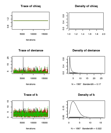
posterior distribution with adequate mixing (note it is really only k that we are interested in):
- Trace and density plots
View codeConclusion:
plot(as.mcmc(plant.r2jags))

- Raftery diagnostic
View codeConclusion:
raftery.diag(as.mcmc(plant.r2jags))
[[1]]

Quantile (q) = 0.025
Accuracy (r) = +/- 0.005
Probability (s) = 0.95

You need a sample size of at least 3746 with these values of q, r and s

[[2]]

Quantile (q) = 0.025
Accuracy (r) = +/- 0.005
Probability (s) = 0.95

You need a sample size of at least 3746 with these values of q, r and s

[[3]]

Quantile (q) = 0.025
Accuracy (r) = +/- 0.005
Probability (s) = 0.95

You need a sample size of at least 3746 with these values of q, r and s
- Autocorrelation
View codeConclusion:
autocorr.diag(as.mcmc(plant.r2jags))
        chisq  deviance         k resid[1] resid[2]
Lag 0     NaN  1.000000  1.000000      NaN      NaN
Lag 10    NaN -0.019121  0.009926      NaN      NaN
Lag 50    NaN  0.013140  0.033150      NaN      NaN
Lag 100   NaN -0.009105  0.018748      NaN      NaN
Lag 500   NaN -0.010926 -0.016835      NaN      NaN
- Trace and density plots
- What conclusions would you draw?
- Lets now extend this fictitious endeavor. Recent studies on a related species of shrub have suggested a 30:70 female:male sex ratio.
Knowing that our plant ecologist had similar research interests, the authors contacted her to inquire whether her data contradicted their findings.
Fit the appropriate JAGS (BUGS) model. We can reuse the JAGS model from above. We just have to alter the expected values (input data) and rerun the analysis.
Show code
plant.list2 <- list(obs=c(40,50),exp=c(27,63), n=2)
plant.r2jags2 <- jags(data=plant.list2,
          inits=NULL, #or inits=list(inits,inits,inits) # since there are three chains
          parameters.to.save=params,
          model.file="../downloads/BUGSscripts/ws11.2bQ1.1.txt",
          n.chains=3,
          n.iter=nIter,
          n.burnin=burnInSteps,
      n.thin=thinSteps
          )
Compiling data graph
   Resolving undeclared variables
   Allocating nodes
   Initializing
   Reading data back into data table
Compiling model graph
   Resolving undeclared variables
   Allocating nodes
   Graph Size: 11

Initializing model
print(plant.r2jags2)
Inference for Bugs model at "../downloads/BUGSscripts/ws11.2bQ1.1.txt", fit using jags, 3 chains, each with 16667 iterations (first 1000 discarded), n.thin = 10 n.sims = 4701 iterations saved mu.vect sd.vect 2.5% 25% 50% 75% 97.5% Rhat n.eff chisq 8.942 0.00 8.942 8.942 8.942 8.942 8.942 1.000 1 k 10.886 4.24 3.574 7.901 10.557 13.572 19.964 1.001 4700 resid[1] 6.259 0.00 6.259 6.259 6.259 6.259 6.259 1.000 1 resid[2] 2.683 0.00 2.683 2.683 2.683 2.683 2.683 1.000 1 deviance 5.686 1.40 4.704 4.800 5.141 6.030 9.648 1.001 3500 For each parameter, n.eff is a crude measure of effective sample size, and Rhat is the potential scale reduction factor (at convergence, Rhat=1). DIC info (using the rule, pD = var(deviance)/2) pD = 1.0 and DIC = 6.7 DIC is an estimate of expected predictive error (lower deviance is better). - What conclusions would you draw from this analysis?
- We could alternatively explore these data from the perspective of estimating the population fractions given the observed data.
We do this by fitting a binomial model:
\begin{align*}
obs_i &\sim Bin(p_i,n_i)\\
p_i &\sim B(a_i,b_i)\\
a &\sim gamma(1, 0.01)\\
b &\sim gamma(1, 0.01)
\end{align*}
where $p_i$ are the probabilities (fractions) of each sex, $n_i$ are the total number of individuals and $a_i$ and $b_i$
are hyper parameters of the prior beta distribution. Have a go at specifying the model in JAGS.
Show code
modelString="
model {
  #Likelihood
 for (i in 1:nGroups) {
   obs[i] ~ dbin(p[i],n[i])
   p[i] ~ dbeta(a[i],b[i])
   a[i] ~ dgamma(1,0.01)
   b[i] ~ dgamma(1,0.01)
 }
 }
"
## write the model to a text file (I suggest you alter the path to somewhere more relevant
## to your system!)
writeLines(modelString,con="../downloads/BUGSscripts/ws11.2bQ1.9.txt")
-
Next create a suitable data list incorporating the observed values ($obs$), the total number of species ($n$) and the number of sexes ($nGroups$).
Show code
obs <- c(40, 50)
plant.list3 <- list(obs = obs, n = c(90, 90), nGroups = 2)
plant.list3
$obs
[1] 40 50

$n
[1] 90 90

$nGroups
[1] 2
-
Define the MCMC chain parameters (similar to above) along with the nodes to monitor (just the two $p$ parameter values).
Show code
params <- c("p")
nChains = 3
burnInSteps = 1000
thinSteps = 10
numSavedSteps = 5000
nIter = ceiling((numSavedSteps * thinSteps)/nChains)
- Now fit the model via the R2jags interface.
Show code
plant.r2jags3 <- jags(data=plant.list3,
          inits=NULL, #or inits=list(inits,inits,inits) # since there are three chains
          parameters.to.save=params,
          model.file="../downloads/BUGSscripts/ws11.2bQ1.9.txt",
          n.chains=3,
          n.iter=nIter,
          n.burnin=burnInSteps,
      n.thin=thinSteps
          )
Compiling model graph
   Resolving undeclared variables
   Allocating nodes
   Graph Size: 13

Initializing model
print(plant.r2jags3)
Inference for Bugs model at "../downloads/BUGSscripts/ws11.2bQ1.9.txt", fit using jags, 3 chains, each with 16667 iterations (first 1000 discarded), n.thin = 10 n.sims = 4701 iterations saved mu.vect sd.vect 2.5% 25% 50% 75% 97.5% Rhat n.eff p[1] 0.447 0.053 0.348 0.411 0.446 0.484 0.551 1.001 3800 p[2] 0.555 0.052 0.450 0.521 0.555 0.591 0.656 1.001 3500 deviance 11.930 2.045 9.947 10.506 11.283 12.711 17.317 1.002 2200 For each parameter, n.eff is a crude measure of effective sample size, and Rhat is the potential scale reduction factor (at convergence, Rhat=1). DIC info (using the rule, pD = var(deviance)/2) pD = 2.1 and DIC = 14.0 DIC is an estimate of expected predictive error (lower deviance is better). - Confirm that the MCMC sampler converged and mixed well
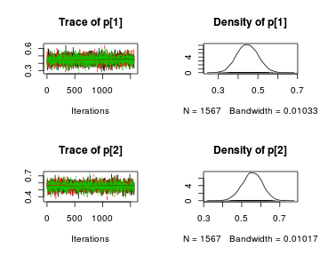
Show code
library(plyr)
library(coda)
preds <- c("p[1]", "p[2]")
# Trace and density plots
plot(as.mcmc.list(alply(plant.r2jags3$BUGSoutput$sims.array[, , preds], 2, function(x) {
    as.mcmc(x)
})))
autocorr.diag(as.mcmc.list(alply(plant.r2jags3$BUGSoutput$sims.array[, , preds], 2, function(x) {
    as.mcmc(x)
})))
            p[1]       p[2]
Lag 0  1.0000000  1.0000000
Lag 1  0.0567558  0.0544404
Lag 5  0.0133714  0.0063118
Lag 10 0.0006573 -0.0007803
Lag 50 0.0056291 -0.0304791
raftery.diag(as.mcmc(plant.r2jags3))
[[1]]

Quantile (q) = 0.025
Accuracy (r) = +/- 0.005
Probability (s) = 0.95

You need a sample size of at least 3746 with these values of q, r and s

[[2]]

Quantile (q) = 0.025
Accuracy (r) = +/- 0.005
Probability (s) = 0.95

You need a sample size of at least 3746 with these values of q, r and s

[[3]]

Quantile (q) = 0.025
Accuracy (r) = +/- 0.005
Probability (s) = 0.95

You need a sample size of at least 3746 with these values of q, r and s
- What conclusions would you draw from the above analyses?
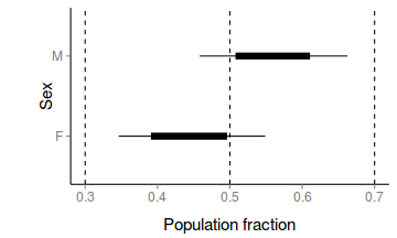
Comment on whether a 1:1 (0.5:0.5) or 30:70 (0.3:0.7) ratios are likely.
- How about a nice summary figure?
Show code
preds <- c("p[1]", "p[2]")
plant.mcmc <- as.mcmc(plant.r2jags3$BUGSoutput$sims.matrix[, preds])
head(plant.mcmc)
Markov Chain Monte Carlo (MCMC) output:
Start = 1
End = 7
Thinning interval = 1
       p[1]   p[2]
[1,] 0.4547 0.5936
[2,] 0.3620 0.5323
[3,] 0.4258 0.5913
[4,] 0.5615 0.5523
[5,] 0.4348 0.4841
[6,] 0.5217 0.5361
[7,] 0.4194 0.6397
plant.mcmc.sum <- adply(plant.mcmc, 2, function(x) { data.frame(mean = mean(x), median = median(x), coda:::HPDinterval(x, p = c(0.68)), coda:::HPDinterval(x)) }) plant.mcmc.sum$Sex = c("F", "M") murray_theme <- theme(panel.grid.major = element_blank(), panel.grid.minor = element_blank(), panel.border = element_blank(), panel.background = element_blank(), axis.title.y = element_text(size = 15, vjust = 0, angle = 90), axis.text.y = element_text(size = 12), axis.title.x = element_text(size = 15, vjust = -1), axis.text.x = element_text(size = 12), axis.line = element_line(), legend.position = c(1, 0.1), legend.justification = c(1, 0), legend.key = element_blank(), plot.margin = unit(c(0.5, 0.5, 1, 2), "lines")) library(ggplot2) p <- ggplot(plant.mcmc.sum, aes(y = mean, x = Sex)) + geom_hline(yintercept = 0.5, linetype = "dashed") + geom_hline(yintercept = c(0.3, 0.7), linetype = "dashed") + geom_errorbar(aes(ymin = lower.1, ymax = upper.1, x = Sex), width = 0) + geom_errorbar(aes(ymin = lower, ymax = upper, x = Sex), width = 0, size = 3) + scale_y_continuous("Population fraction") + geom_point() + coord_flip() + murray_theme p
