Tutorial 11.4b -Logistic regression
05 Sep 2016
Binary data
Scenario and Data
Logistic regression is a type of generalized linear model (GLM) that models a binary response against a linear predictor via a specific link function. The linear predictor is the typically a linear combination of effects parameters (e.g. $\beta_0 + \beta_1x_x$). The role of the link function is to transform the expected values of the response y (which is on the scale of (0,1), as is the binomial distribution from which expectations are drawn) into the scale of the linear predictor (which is $-\infty,\infty$). GLM's transform the expected values (via a link) whereas LM's transform the observed data. Thus while GLM's operate on the scale of the original data and yet also on a scale appropriate of the residuals, LM's do neither.
There are many ways (transformations) that can map values on the (0,1) scale into values on the ($-\infty,\infty$) scale, however, the three most common are:
- logit: $log\left(\frac{\pi}{1-\pi}\right)$ - log odds ratio
- probit: $\phi^{-1}(\pi)$ where $\phi^{-1}$ is an inverse normal cumulative density function
- complimentary log-log: $log(-log(1-\pi))$
Lets say we wanted to model the presence/absence of an item ($y$) against a continuous predictor ($x$) As this section is mainly about the generation of artificial data (and not specifically about what to do with the data), understanding the actual details are optional and can be safely skipped. Consequently, I have folded (toggled) this section away.
- the sample size = 20
- the continuous $x$ variable is a random uniform spread of measurements between 1 and 20
- the rate of change in log odds ratio per unit change in x (slope) = 0.5. The magnitude of the slope is an indicator of how abruptly the log odds ratio changes. A very abrupt change would occur if there was very little variability in the trend. That is, a large slope would be indicative of a threshold effect. A lower slope indicates a gradual change in odds ratio and thus a less obvious and precise switch between the likelihood of 1 vs 0.
- the inflection point (point where the slope of the line is greatest) = 10. The inflection point indicates the value of the predictor ($x$) where the log Odds are 50% (switching between 1 being more likely and 0 being more likely). This is also known as the LD50.
- the intercept (which has no real interpretation) is equal to the negative of the slope multiplied by the inflection point
- to generate the values of $y$ expected at each $x$ value, we evaluate the linear predictor. These expected values are then transformed into a scale mapped by (0,1) by using the inverse logit function $\frac{e^{linear~predictor}}{1+e^{linear~predictor}}$
- finally, we generate $y$ values by using the expected $y$ values as probabilities when drawing random numbers from a binomial distribution. This step adds random noise to the expected $y$ values and returns only 1's and 0's.
set.seed(8)
#The number of samples
n.x <- 20
#Create x values that at uniformly distributed throughout the rate of 1 to 20
x <- sort(runif(n = n.x, min = 1, max =20))
#The slope is the rate of change in log odds ratio for each unit change in x
# the smaller the slope, the slower the change (more variability in data too)
slope=0.5
#Inflection point is where the slope of the line is greatest
#this is also the LD50 point
inflect <- 10
#Intercept (no interpretation)
intercept <- -1*(slope*inflect)
#The linear predictor
linpred <- intercept+slope*x
#Predicted y values
y.pred <- exp(linpred)/(1+exp(linpred))
#Add some noise and make binomial
n.y <-rbinom(n=n.x,20,p=0.9)
y<- rbinom(n = n.x,size=1, prob = y.pred)
dat <- data.frame(y,x)
With these sort of data, we are primarily interested in investigating whether there is a relationship between the binary response variable and the linear predictor (linear combination of one or more continuous or categorical predictors).
Exploratory data analysis and initial assumption checking
- All of the observations are independent - this must be addressed at the design and collection stages
- The response variable (and thus the residuals) should be matched by an appropriate distribution (in the case of a binary response - a binomial is appropriate).
- All observations are equally influential in determining the trends - or at least no observations are overly influential. This is most effectively diagnosed via residuals and other influence indices and is very difficult to diagnose prior to analysis
- the relationship between the linear predictor (right hand side of the regression formula) and the link function should be linear. A scatterplot with smoother can be useful for identifying possible non-linearity.
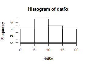
So lets explore linearity by creating a histogram of the predictor variable ($x$) and a scatterplot of the relationship between the response ($y$) and the predictor ($x$)
hist(dat$x)
#now for the scatterplot
plot(y~x, dat)
with(dat, lines(lowess(y~x)))
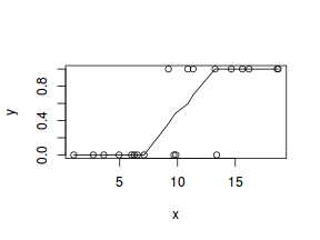
Conclusions: the predictor ($x$) does not display any skewness or other issues that might lead to non-linearity. The lowess smoother on the scatterplot does not display major deviations from a standard sigmoidal curve and thus linearity is satisfied. Violations of linearity could be addressed by either:
- define a non-linear linear predictor (such as a polynomial, spline or other non-linear function)
- transform the scale of the predictor variables
JAGS
Effects model
Note that in order to prevent arithmetic overflows (particularly with the clog-log model, I am going to constrain the estimated linear predictor to between -20 and 20. Values outside of this on a inverse-log scale are extremely small and huge respectively.I will demonstrate logistic regression with a range of possible link functions (each of which yield different parameter interpretations):
- logit
$$
\begin{array}{rcl}
y &\sim& \operatorname{Bern}(\pi)\\
log\left(\frac{\pi}{1-\pi}\right)&=&\beta_0+\beta_1x_1\\
\beta_0, \beta_1&\sim&\mathcal{N}(0, 10000)\\
\end{array}
$$
dat.list <- with(dat, list(y=y, x=x, N=nrow(dat)))
modelString="
model{
  for (i in 1:N) {
    y[i] ~ dbern(p[i])
    logit(p[i]) <- max(-20,min(20,beta0+beta1*x[i]))
  }
  beta0 ~ dnorm(0,1.0E-06)
  beta1 ~ dnorm(0,1.0E-06)
}
"
writeLines(modelString, con='../downloads/BUGSscripts/tut11.4bS1.bug')
library(R2jags)
dat.logit.jags <- jags(data=dat.list,model.file='../downloads/BUGSscripts/tut11.4bS1.bug',
                   param=c('beta0','beta1'),
                   n.chains=3, n.iter=20000, n.burnin=10000, n.thin=10)
Compiling model graph
   Resolving undeclared variables
   Allocating nodes
   Graph Size: 147

Initializing model
- probit
$$
\begin{array}{rcl}
y &\sim& \operatorname{Bern}(\pi)\\
\phi^{-1}\left(\pi\right)&=&\beta_0+\beta_1x_1\\
\beta_0, \beta_1&\sim&\mathcal{N}(0, 10000)\\
\end{array}
$$
dat.list <- with(dat, list(y=y, x=x, N=nrow(dat)))
modelString="
model{
  for (i in 1:N) {
    y[i] ~ dbern(p[i])
    probit(p[i]) <- max(-20,min(20,beta0+beta1*x[i]))
  }
  beta0 ~ dnorm(0,1.0E-06)
  beta1 ~ dnorm(0,1.0E-06)
}
"
writeLines(modelString, con='../downloads/BUGSscripts/tut11.4bS1.3b.bug')
library(R2jags)
dat.probit.jags <- jags(data=dat.list,model.file='../downloads/BUGSscripts/tut11.4bS1.3b.bug',
                   param=c('beta0','beta1'),
                   n.chains=3, n.iter=20000, n.burnin=10000, n.thin=10)
Compiling model graph
   Resolving undeclared variables
   Allocating nodes
   Graph Size: 147

Initializing model
- complimentary log-log
$$
\begin{array}{rcl}
y &\sim& \operatorname{Bern}(\pi)\\
log(-log(1-\pi))&=&\beta_0+\beta_1x_1\\
\beta_0, \beta_1&\sim&\mathcal{N}(0, 10000)\\
\end{array}
$$
dat.list <- with(dat, list(y=y, x=x, N=nrow(dat)))
modelString="
model{
  for (i in 1:N) {
    y[i] ~ dbern(p[i])
    cloglog(p[i]) <- max(-20,min(20,beta0+beta1*x[i]))
  }
  beta0 ~ dnorm(0,1.0E-06)
  beta1 ~ dnorm(0,1.0E-06)
}
"
writeLines(modelString, con='../downloads/BUGSscripts/tut11.4bS1.3c.bug')
library(R2jags)
dat.cloglog.jags <- jags(data=dat.list,model.file='../downloads/BUGSscripts/tut11.4bS1.3c.bug',
                   param=c('beta0','beta1'),
                   n.chains=3, n.iter=20000, n.burnin=10000, n.thin=10)
Compiling model graph
   Resolving undeclared variables
   Allocating nodes
   Graph Size: 147

Initializing model
dat.glmC <- glm(y~x, data=dat, family=binomial(link="cloglog"))
Chain mixing and Model validation
Prior to exploring the model parameters, it is prudent to confirm that the model did indeed fit the assumptions and was an appropriate fit to the data as well as that the MCMC sampling chain was adequately mixed and the retained samples independent.
Whilst I will only demonstrate this for the logit model, the procedure would be identical for exploring the probit and clog-log models.
- We will start by exploring the mixing of the MCMC chains via traceplots.
plot(as.mcmc(dat.logit.jags))
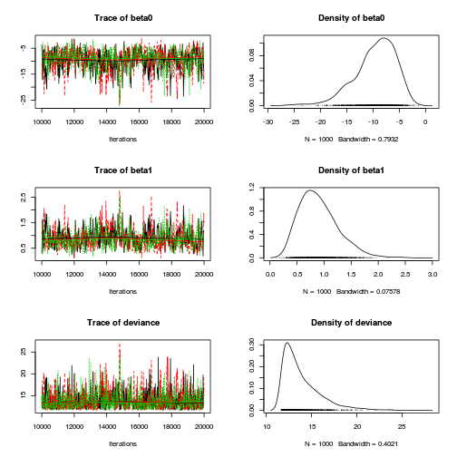
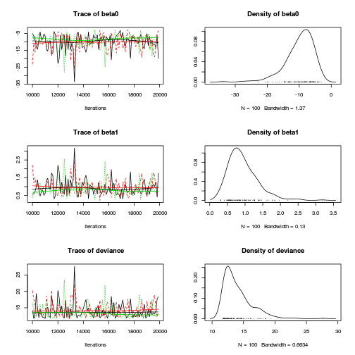
Other than the large spike in one of the chains (not ideal), the chains appear well mixed. Nevertheless, it is clear that the parameters are not symmetrically distributed. Hence, medians might be better descriptors of parameter estimates than means.
- Next we will explore correlation amongst MCMC samples.
autocorr.diag(as.mcmc(dat.logit.jags))
          beta0   beta1 deviance
Lag 0   1.00000 1.00000  1.00000
Lag 10  0.73921 0.74013  0.38068
Lag 50  0.23896 0.23575  0.12992
Lag 100 0.02871 0.04098  0.04769
Lag 500 0.01573 0.01148  0.01980
It seems that the level of auto-correlation at the nominated lag of 10 is extremely high. Ideally, the level of auto-correlation should be less than 0.1. To achieve this, we need a lag of 1000. Consequently, we will resample at a lag of 1000 and obviously we are going to need more iterations to ensure that we retain a large enough sample from which to derive estimates.
In order to support a thinning rate of 1000, the number of iterations is going to need to be very high. Hence, the following might take considerable time to run.
library(R2jags)
dat.logit.jags <- jags(data=dat.list,model.file='../downloads/BUGSscripts/tut11.4bS1.bug',
                   param=c('beta0','beta1'),
                   n.chains=3, n.iter=20000, n.burnin=10000, n.thin=100)
Compiling model graph
   Resolving undeclared variables
   Allocating nodes
   Graph Size: 147

Initializing model
plot(as.mcmc(dat.logit.jags))
autocorr.diag(as.mcmc(dat.logit.jags))
            beta0    beta1  deviance
Lag 0     1.00000  1.00000  1.000000
Lag 100   0.09970  0.12296  0.131321
Lag 500  -0.01581 -0.02810 -0.003366
Lag 1000  0.06601  0.05309 -0.008802
Lag 5000 -0.01542 -0.03085 -0.013968
Conclusions: the samples are now less auto-correlated and the chains are arguably mixed better.
- We now explore the goodness of fit of the models via the residuals and deviance.
We could calculate the Pearsons's residuals within the JAGS model.
Alternatively, we could use the parameters to generate the residuals outside of JAGS.
coefs <- dat.logit.jags$BUGSoutput$sims.matrix[,1:2]
Xmat <- model.matrix(~x, data=dat)
eta<-coefs %*% t(Xmat)
pi <- inv.logit(eta)
#sweep across rows and then divide by pi
Resid <- -1*sweep(pi,2,dat$y,'-')/sqrt(pi*(1-pi))
plot(apply(Resid,2,mean)~apply(eta,2,mean))

- Now we will compare the sum of squared residuals to the sum of squares residuals that would be expected from a Bernoulli distribution
matching that estimated by the model. Essentially this is estimating how well the Bernoulli distribution and linear model
approximates the observed data.
Alternatively, we could generate the new samples and calculate the sums squares of residuals etc all within JAGS.
SSres<-apply(Resid^2,1,sum)

set.seed(2)
#generate a matrix of draws from a binomial distribution
# the matrix is the same dimensions as pi and uses the probabilities of pi
YNew <- matrix(rbinom(length(pi),prob=pi,size=1),nrow=nrow(pi))

Resid1<-(pi - YNew)/sqrt(pi*(1-pi))
SSres.sim<-apply(Resid1^2,1,sum)
mean(SSres.sim>SSres)
[1] 0.23
dat.list <- with(dat, list(y=y, x=x, N=nrow(dat)))
modelString="
model{
  for (i in 1:N) {
    y[i] ~ dbern(p[i])
    logit(p[i]) <- max(-20,min(20,eta[i]))
    eta[i] <- beta0+beta1*x[i]
    YNew[i] ~dbern(p[i])
    varY[i] <- p[i]*(1-p[i])
    PRes[i] <- (y[i] - p[i]) / sqrt(varY[i])
    PResNew[i] <- (YNew[i] - p[i]) / sqrt(varY[i])
    D[i] <- pow(PRes[i],2)
    DNew[i] <- pow(PResNew[i],2)
  }
  Fit <- sum(D[1:N])
  FitNew <-sum(DNew[1:N])
  beta0 ~ dnorm(0,1.0E-06)
  beta1 ~ dnorm(0,1.0E-06)
  pvalue <- mean(FitNew>Fit)
}
"
writeLines(modelString, con='../downloads/BUGSscripts/tut11.4bS5.bug')
library(R2jags)
dat.logit.jags1 <- jags(data=dat.list,model.file='../downloads/BUGSscripts/tut11.4bS5.bug',
                   param=c('beta0','beta1','Fit','FitNew'),
                   n.chains=3, n.iter=20000, n.burnin=10000, n.thin=10)
Compiling model graph
   Resolving undeclared variables
   Allocating nodes
   Graph Size: 346

Initializing model
print(dat.logit.jags1)
Inference for Bugs model at "../downloads/BUGSscripts/tut11.4bS5.bug", fit using jags,
 3 chains, each with 20000 iterations (first 10000 discarded), n.thin = 10
 n.sims = 3000 iterations saved
         mu.vect sd.vect    2.5%     25%    50%
Fit       92.725 700.607   9.931  13.217 20.734
FitNew    17.011  45.964   1.607   4.049  7.838
beta0     -9.721   4.274 -19.899 -11.975 -9.110
beta1      0.915   0.402   0.323   0.630  0.860
deviance  14.004   2.309  11.710  12.378 13.323
            75%   97.5%  Rhat n.eff
Fit      40.679 381.579 1.016   300
FitNew   16.322  78.923 1.003   760
beta0    -6.620  -3.430 1.011   330
beta1     1.128   1.892 1.008   310
deviance 14.908  20.337 1.012   390

For each parameter, n.eff is a crude measure of effective sample size,
and Rhat is the potential scale reduction factor (at convergence, Rhat=1).

DIC info (using the rule, pD = var(deviance)/2)
pD = 2.7 and DIC = 16.7
DIC is an estimate of expected predictive error (lower deviance is better).
out <- dat.logit.jags1$BUGSoutput mean(out$sims.list$FitNew > out$sims.list$Fit)
[1] 0.244
Conclusions: although the Bayesian p-value is quite a bit lower than 0.5, suggesting that there is more variability in the data than should be expected from this simple logistic regression model, this value is not any closer to 0 (a value that would indicate that the model does not fit the data at all well. Thus we might conclude that whilst not ideal, the model is adequate.
Exploring the model parameters, test hypotheses
If there was any evidence that the assumptions had been violated or the model was not an appropriate fit, then we would need to reconsider the model and start the process again. In this case, there is no evidence that the test will be unreliable so we can proceed to explore the test statistics.
print(dat.logit.jags)
Inference for Bugs model at "../downloads/BUGSscripts/tut11.4bS1.bug", fit using jags,
 3 chains, each with 20000 iterations (first 10000 discarded), n.thin = 100
 n.sims = 300 iterations saved
         mu.vect sd.vect    2.5%     25%    50%
beta0     -9.898   4.468 -20.384 -12.214 -9.110
beta1      0.941   0.425   0.324   0.638  0.859
deviance  14.073   2.294  11.736  12.364 13.398
            75%  97.5%  Rhat n.eff
beta0    -6.796 -3.839 1.022   100
beta1     1.152  1.913 1.016   120
deviance 14.988 19.460 1.016   100

For each parameter, n.eff is a crude measure of effective sample size,
and Rhat is the potential scale reduction factor (at convergence, Rhat=1).

DIC info (using the rule, pD = var(deviance)/2)
pD = 2.6 and DIC = 16.7
DIC is an estimate of expected predictive error (lower deviance is better).
library(plyr)
adply(dat.logit.jags$BUGSoutput$sims.matrix[,1:2], 2, function(x) {
  data.frame(Median=median(x), Mean=mean(x), HPDinterval(as.mcmc(x)), HPDinterval(as.mcmc(x),p=0.5))
})
     X1  Median    Mean    lower  upper  lower.1
1 beta0 -9.1101 -9.8980 -18.3513 -2.815 -10.2669
2 beta1  0.8593  0.9405   0.2807  1.778   0.5729
  upper.1
1  -5.658
2   1.013
Conclusions:
We would reject the null hypothesis (p<0.05).
An increase in x is associated with a significant linear increase (positive slope) in log odds of $y$ success.
Every 1 unit increase in $x$ results in a 0.8593198 unit increase in log odds-ratio.
We usually express this in terms of odds-ratio rather than log odds-ratio, so
every 1 unit increase in $x$ results in a ($e^{0.8593198}=2.3615537$)
2.3615537 unit increase in odds-ratio.
Further explorations of the trends
We might also be interested in the LD50 - the value of $x$ where the probability switches from favoring 1 to favoring 0. LD50 is calculated as: $$LD50 = - \frac{intercept}{slope}$$
library(coda)
summary(as.mcmc(-coefs[,1]/coefs[,2]))
Iterations = 1:300
Thinning interval = 1
Number of chains = 1
Sample size per chain = 300

1. Empirical mean and standard deviation for each variable,
   plus standard error of the mean:

          Mean             SD       Naive SE
      10.59179        1.09415        0.06317
Time-series SE
       0.04197

2. Quantiles for each variable:

  2.5%    25%    50%    75%  97.5%
 8.684  9.898 10.495 11.223 12.970
#OR
LD50 <- -coefs[,1]/coefs[,2]
data.frame(Median=median(LD50), Mean=mean(LD50), HPDinterval(as.mcmc(LD50)), HPDinterval(as.mcmc(LD50),p=0.5))
       Median     Mean    lower    upper  lower.1
var1 10.49471 10.59179 8.495029 12.73212 9.646387
      upper.1
var1 10.87609
10.4947098.
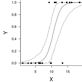
Finally, we will create a summary plot.
par(mar = c(4, 5, 0, 0))
plot(y ~ x, data = dat, type = "n", ann = F, axes = F)
points(y ~ x, data = dat, pch = 16)
xs <- seq(0, 20, l = 1000)

Xmat <- model.matrix(~xs)
eta<-coefs %*% t(Xmat)
library(boot)
ys <- inv.logit(eta)
library(plyr)
data.tab <- adply(ys,2,function(x) {
  data.frame(Median=median(x), HPDinterval(as.mcmc(x)))
})
data.tab <- cbind(x=xs,data.tab)

points(Median ~ x, data=data.tab,col = "black", type = "l")
lines(lower ~ x, data=data.tab,col = "black", type = "l", lty = 2)
lines(upper ~ x, data=data.tab,col = "black", type = "l", lty = 2)
axis(1)
mtext("X", 1, cex = 1.5, line = 3)
axis(2, las = 2)
mtext("Y", 2, cex = 1.5, line = 3)
box(bty = "l")
Grouped binary data (and proportional data)
Scenario and Data
In the previous demonstration, the response variable represented the state of a single item per level of the predictor variable ($x$). That single item could be observed having a value of either 1 or 0. Another common situation is to observe the number of items in one of two states (typically dead or alive) for each level of a treatment. For example, you could tally up the number of germinated and non-germinated seeds out of a bank of 10 seeds at each of 8 temperature or nutrient levels.
Recall that the binomial distribution represents the density (probability) of all possible successes (germinations) out of a total of $N$ items (seeds). Hence the binomial distribution is also a suitable error distribution for such grouped binary data.
For this demonstration, we will model the number of successes against a uniformly distributed predictor ($x$). The number of trials in each group (level of the predictor) will vary slightly (yet randomly) so as to mimick complications that inevadably occur in real experimentws.
- the number of levels of $x$ = 10
- the continuous $x$ variable is a random uniform spread of measurements between 10 and 20
- the rate of change in log odds ratio per unit change in x (slope) = -0.25. The magnitude of the slope is an indicator of how abruptly the log odds ratio changes. A very abrupt change would occur if there was very little variability in the trend. That is, a large slope would be indicative of a threshold effect. A lower slope indicates a gradual change in odds ratio and thus a less obvious and precise switch between the likelihood of 1 vs 0.
- the inflection point (point where the slope of the line is greatest) = 10. The inflection point indicates the value of the predictor ($x$) where the log Odds are 50% (switching between 1 being more likely and 0 being more likely). This is also known as the LD50.
- the intercept (which has no real interpretation) is equal to the negative of the slope multiplied by the inflection point
- generate the values of $y$ expected at each $x$ value, we evaluate the linear predictor.
- generate random numbers of trials per group by drawing integers out of a binomial distribution with a total size of 20 and probability of 0.9. Hence the maximum number of trials per group will be 20, yet some will be less than that.
- the number of success per group are drawn from a binomial distribution with a total size equal to the trial sizes generated in the previous step and probabilities equal to the expected $y$ values
- finally, the number of failures per group are calculated as the difference between the total trial size and number of successes per group.
set.seed(8)
#The number of levels of x
n.x <- 10
#Create x values that at uniformly distributed throughout the rate of 10 to 20
x <- sort(runif(n = n.x, min = 10, max =20))
#The slope is the rate of change in log odds ratio for each unit change in x
# the smaller the slope, the slower the change (more variability in data too)
slope=-.25
#Inflection point is where the slope of the line is greatest
#this is also the LD50 point
inflect <- 15
#Intercept (no interpretation)
intercept <- -1*(slope*inflect)
#The linear predictor
linpred <- intercept+slope*x
#Predicted y values
y.pred <- exp(linpred)/(1+exp(linpred))
#Add some noise and make binary (0's and 1's)
n.trial <- rbinom(n=n.x,20, prob=0.9)
success <- rbinom(n = n.x, size = n.trial,prob = y.pred)
failure <- n.trial - success
dat <- data.frame(success,failure,x)
Exploratory data analysis and initial assumption checking
- All of the observations are independent - this must be addressed at the design and collection stages
- The response variable (and thus the residuals) should be matched by an appropriate distribution (in the case of a binary response - a binomial is appropriate).
- All observations are equally influential in determining the trends - or at least no observations are overly influential. This is most effectively diagnosed via residuals and other influence indices and is very difficult to diagnose prior to analysis
- the relationship between the linear predictor (right hand side of the regression formula) and the link function should be linear. A scatterplot with smoother can be useful for identifying possible non-linearity.
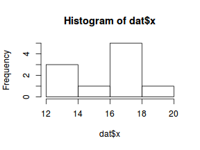
So lets explore linearity by creating a histogram of the predictor variable ($x$) and a scatterplot of the relationship between the either the number of successes ($success$) or the number of ($failures$) and the predictor ($x$). Note, that this will not account for the differences in trial size per group and so a scatterplot of the relationship between the number of successes ($success$) or the number of ($failures$) divided by the total number of trials against the predictor ($x$) might be more appropriate.
hist(dat$x)
#now for the scatterplot
plot(success~x, dat)
with(dat, lines(lowess(success~x)))
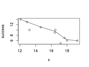
#scatterplot standardized for trial size
plot(success/(success+failure)~x, dat)
with(dat, lines(lowess(success/(success+failure)~x)))
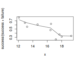
Conclusions: the predictor ($x$) does not display any skewness (although it is not all that uniform - random data hey!) or other issues that might lead to non-linearity. The lowess smoother on either scatterplot does not display major deviations from a standard sigmoidal curve and thus linearity is likely to be satisfied. Violations of linearity could be addressed by either:
- define a non-linear linear predictor (such as a polynomial, spline or other non-linear function)
- transform the scale of the predictor variables
Model fitting or statistical analysis - JAGS
Clearly the number of successes is also dependent on the number of trials. Larger numbers of trials might be expected to yeild higher numbers of successes.
dat.list <- with(dat, list(success=success, total=success+failure, x=x, N=nrow(dat)))
modelString="
model{
  for (i in 1:N) {
    success[i] ~ dbin(p[i],total[i])
    logit(p[i]) <- max(-20,min(20,beta0+beta1*x[i]))
  }
  beta0 ~ dnorm(0,1.0E-06)
  beta1 ~ dnorm(0,1.0E-06)
}
"
writeLines(modelString, con='../downloads/BUGSscripts/tut11.4bS2.bug')
library(R2jags)
dat.logit.jags <- jags(data=dat.list,model.file='../downloads/BUGSscripts/tut11.4bS2.bug',
                   param=c('beta0','beta1'),
                   n.chains=3, n.iter=200000, n.burnin=100000, n.thin=100)
Compiling model graph
   Resolving undeclared variables
   Allocating nodes
   Graph Size: 87

Initializing model
As with the logistic regression presented earlier, we could alternatively use probit or clog-log link functions.
Model evaluation
Prior to exploring the model parameters, it is prudent to confirm that the model did indeed fit the assumptions and was an appropriate fit to the data.
- We will start by exploring the mixing of the MCMC chains via traceplots.
plot(as.mcmc(dat.logit.jags))
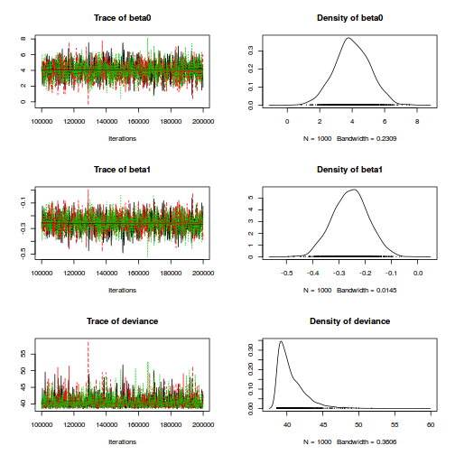
Conclusions: the chains appear well mixed and stable.
- Next we will explore correlation amongst MCMC samples.
autocorr.diag(as.mcmc(dat.logit.jags))
                beta0        beta1     deviance
Lag 0     1.000000000  1.000000000  1.000000000
Lag 100   0.237750449  0.243869665  0.025807991
Lag 500   0.005225247  0.007250363  0.008398106
Lag 1000 -0.007840742 -0.009143387 -0.028934638
Lag 5000 -0.004896295 -0.004932879 -0.027304575
It seems that the level of auto-correlation at the nominated lag of 10 is extremely high. Ideally, the level of auto-correlation should be less than 0.1. To achieve this, we need a lag of 100. Consequently, we will resample at a lag of 100 and obviously we are going to need more iterations to ensure that we retain a large enough sample from which to derive estimates.
library(R2jags)
dat.logit.jags <- jags(data=dat.list,model.file='../downloads/BUGSscripts/tut11.4bS2.bug',
                   param=c('beta0','beta1'),
                   n.chains=3, n.iter=2000000, n.burnin=10000, n.thin=1000)
Compiling model graph
   Resolving undeclared variables
   Allocating nodes
   Graph Size: 87

Initializing model
plot(as.mcmc(dat.logit.jags))
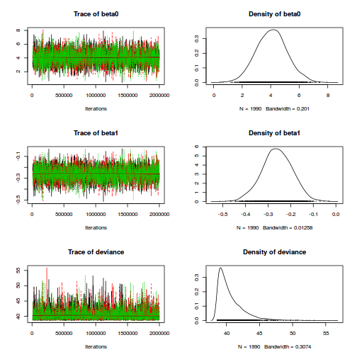
autocorr.diag(as.mcmc(dat.logit.jags))
                 beta0        beta1     deviance
Lag 0      1.000000000  1.000000000  1.000000000
Lag 1000  -0.009933648 -0.010646679  0.006179711
Lag 5000   0.011433698  0.010182990  0.005045334
Lag 10000 -0.012786987 -0.016708011  0.026831468
Lag 50000  0.006382612  0.003937007 -0.004550967
-
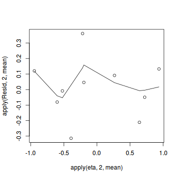
Lets explore the diagnostics - particularly the residuals
Conclusions: there is no obvious patterns in the residuals, or at least there are no obvious trends remaining that would be indicative of non-linearity.inv.logit <- binomial()$linkinv #Calculate residuals coefs <- dat.logit.jags$BUGSoutput$sims.matrix[,1:2] Xmat <- model.matrix(~x, data=dat) eta<-coefs %*% t(Xmat) pi <- inv.logit(eta) #sweep across rows and then divide by pi Resid <- -1*sweep(pi,2,dat$success/(dat$success+dat$failure),'-')/sqrt(pi*(1-pi)) plot(apply(Resid,2,mean)~apply(eta,2,mean)) lines(lowess(apply(Resid,2,mean)~apply(eta,2,mean)))
- Now we will compare the sum of squared residuals to the sum of squares residuals that would be expected from a Bernoulli distribution
matching that estimated by the model. Essentially this is estimating how well the Bernoulli distribution and linear model
approximates the observed data.
SSres<-apply(Resid^2,1,sum)

set.seed(2)
#generate a matrix of draws from a binomial distribution
#the matrix is the same dimensions as pi and uses the probabilities of pi
YNew <- matrix(rbinom(length(pi),prob=pi,size=(dat$success+dat$failure)),nrow=nrow(pi))
Resid1 <- 1*(pi-YNew/(dat$success+dat$failure))/sqrt(pi*(1-pi))
SSres.sim<-apply(Resid1^2,1,sum)
mean(SSres.sim>SSres)
[1] 0.6445561
Conclusions: this Bayesian p-value is reasonably close to 0.5. Therefore we would conclude that there was no strong evidence for a lack of fit of the model.
Further explorations of the trends
We might also be interested in the LD50 - the value of $x$ where the probability switches from favoring 1 to favoring 0. LD50 is calculated as: $$LD50 = - \frac{intercept}{slope}$$
library(coda)
summary(as.mcmc(-coefs[,1]/coefs[,2]))
Iterations = 1:5970
Thinning interval = 1
Number of chains = 1
Sample size per chain = 5970

1. Empirical mean and standard deviation for each variable,
   plus standard error of the mean:

          Mean             SD       Naive SE
     15.672795       0.689132       0.008919
Time-series SE
      0.007972

2. Quantiles for each variable:

 2.5%   25%   50%   75% 97.5%
14.28 15.27 15.68 16.09 16.95
#OR
LD50 <- -coefs[,1]/coefs[,2]
data.frame(Median=median(LD50), Mean=mean(LD50),
           HPDinterval(as.mcmc(LD50)), HPDinterval(as.mcmc(LD50),p=0.5))
       Median     Mean    lower    upper  lower.1
var1 15.67809 15.67279 14.39209 17.04647 15.27153
      upper.1
var1 16.09027
15.6780855.
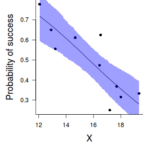
Finally, we will create a summary plot.
par(mar = c(4, 5, 0, 0))
plot(success/(success+failure) ~ x, data = dat, type = "n", ann = F, axes = F)
points(success/(success+failure) ~ x, data = dat, pch = 16)
xs <- seq(min(dat$x, na.rm=TRUE),max(dat$x, na.rm=TRUE), l = 1000)

Xmat <- model.matrix(~xs)
eta<-coefs %*% t(Xmat)
library(boot)
ys <- inv.logit(eta)
library(plyr)
data.tab <- adply(ys,2,function(x) {
  data.frame(Median=median(x), HPDinterval(as.mcmc(x)))
})
data.tab <- cbind(x=xs,data.tab)

points(Median ~ x, data=data.tab,col = "black", type = "l")
with(data.tab,polygon(c(x,rev(x)),c(lower,rev(upper)), col="#0000ff60", border=NA))
#lines(lower ~ x, data=data.tab,col = "black", type = "l", lty = 2)
#lines(upper ~ x, data=data.tab,col = "black", type = "l", lty = 2)
axis(1)
mtext("X", 1, cex = 1.5, line = 3)
axis(2, las = 2)
mtext("Probability of success", 2, cex = 1.5, line = 3)
box(bty = "l")
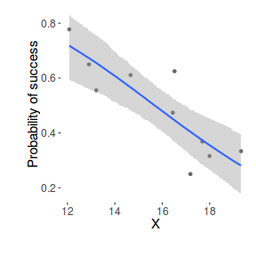
xs <- seq(min(dat$x, na.rm=TRUE),max(dat$x, na.rm=TRUE), l = 1000)
Xmat <- model.matrix(~xs)
eta<-coefs %*% t(Xmat)
library(boot)
ys <- inv.logit(eta)
library(plyr)
data.tab <- adply(ys,2,function(x) {
  data.frame(Median=median(x), HPDinterval(as.mcmc(x)))
})
data.tab <- cbind(x=xs,data.tab)

library(ggplot2)
library(grid)
dat$p <- with(dat, success/(success+failure))
p1 <- ggplot(data.tab,aes(y=Median, x=x)) + geom_point(data=dat,aes(y=p, x=x),color="gray40")+
             geom_smooth(aes(ymin=lower, ymax=upper), stat="identity")+
                         scale_x_continuous("X")+scale_y_continuous("Probability of success")
p1+theme(panel.grid.major=element_blank(),
         panel.grid.minor=element_blank(),
         panel.border=element_blank(),
         panel.background=element_blank(),
                 axis.title.y=element_text(size=15,vjust=0,angle=90),
                 axis.title.x=element_text(size=15,vjust=-1),
                 axis.text.y=element_text(size=12),
                 axis.text.x=element_text(size=12),
                 axis.line=element_line(),
                 plot.margin=unit(c(0.5,0.5,2,2), "lines"))
Worked Examples
Basic χ2 references
- Logan (2010) - Chpt 16-17
- Quinn & Keough (2002) - Chpt 13-14
Logistic regression
Polis et al. (1998) were intested in modelling the presence/absence of lizards (Uta sp.) against the perimeter to area ratio of 19 islands in the Gulf of California.
Download Polis data set| Format of polis.csv data file | |||||||||||||||||||||||||
|---|---|---|---|---|---|---|---|---|---|---|---|---|---|---|---|---|---|---|---|---|---|---|---|---|---|
|

|
polis <- read.table('../downloads/data/polis.csv', header=T, sep=',', strip.white=T)
head(polis)
      ISLAND RATIO PA
1       Bota 15.41  1
2     Cabeza  5.63  1
3    Cerraja 25.92  1
4 Coronadito 15.17  0
5     Flecha 13.04  1
6   Gemelose 18.85  0
- Fit the appropriate logistic regression model
Show JAGS code
modelString="
model
{
  for (i in 1:n) {
	pa[i] ~ dbin(p[i],1)
	logit(p[i]) <- alpha+beta*ratio[i]
  }
	alpha~dnorm(0,1.0E-6)
	beta ~ dnorm(0,1.0E-6)
}
"
## write the model to a text file (I suggest you alter the path to somewhere more relevant
## to your system!)
writeLines(modelString,con="../downloads/BUGSscripts/ws10.5bQ3.1.txt")

polis.list <- with(polis,
                         list(pa=PA,
                         ratio=RATIO,
                         n=nrow(polis))
)


params <- c("alpha","beta")

adaptSteps = 1000
burnInSteps = 2000
nChains = 3
numSavedSteps = 50000
thinSteps = 10
nIter = ceiling((numSavedSteps * thinSteps)/nChains)

polis.r2jags <- jags(data=polis.list,
          inits=NULL,#list(inits,inits,inits), #or inits=list(inits,inits,inits) # since there are three chains
          parameters.to.save=params,
          model.file="../downloads/BUGSscripts/ws10.5bQ3.1.txt",
          n.chains=3,
          n.iter=nIter,
          n.burnin=burnInSteps,
      n.thin=10
          )
Compiling model graph
   Resolving undeclared variables
   Allocating nodes
   Graph Size: 101

Initializing model
print(polis.r2jags)
Inference for Bugs model at "../downloads/BUGSscripts/ws10.5bQ3.1.txt", fit using jags,
 3 chains, each with 166667 iterations (first 2000 discarded), n.thin = 10
 n.sims = 49401 iterations saved
         mu.vect sd.vect   2.5%    25%    50%    75%  97.5%  Rhat n.eff
alpha      4.616   2.034  1.411  3.166  4.345  5.782  9.336 1.001 19000
beta      -0.283   0.122 -0.565 -0.352 -0.267 -0.196 -0.092 1.001 11000
deviance  16.422   2.167 14.279 14.861 15.768 17.274 22.378 1.001 13000

For each parameter, n.eff is a crude measure of effective sample size,
and Rhat is the potential scale reduction factor (at convergence, Rhat=1).

DIC info (using the rule, pD = var(deviance)/2)
pD = 2.3 and DIC = 18.8
DIC is an estimate of expected predictive error (lower deviance is better).
Show BRM codeWe could alternatively center the perimeter-area ratio predictor first. The will help with model convergence and autocorrelation.library(brms)
polis.brm <- brm(PA ~ RATIO, data = polis, family = binomial, prior = c(set_prior("normal(0,100)", class = "b")),
    chains = 3, iter = 2000, warmup = 500, thin = 2)
SAMPLING FOR MODEL 'binomial(logit) brms-model' NOW (CHAIN 1).

Chain 1, Iteration:    1 / 2000 [  0%]  (Warmup)
Chain 1, Iteration:  200 / 2000 [ 10%]  (Warmup)
Chain 1, Iteration:  400 / 2000 [ 20%]  (Warmup)
Chain 1, Iteration:  501 / 2000 [ 25%]  (Sampling)
Chain 1, Iteration:  700 / 2000 [ 35%]  (Sampling)
Chain 1, Iteration:  900 / 2000 [ 45%]  (Sampling)
Chain 1, Iteration: 1100 / 2000 [ 55%]  (Sampling)
Chain 1, Iteration: 1300 / 2000 [ 65%]  (Sampling)
Chain 1, Iteration: 1500 / 2000 [ 75%]  (Sampling)
Chain 1, Iteration: 1700 / 2000 [ 85%]  (Sampling)
Chain 1, Iteration: 1900 / 2000 [ 95%]  (Sampling)
Chain 1, Iteration: 2000 / 2000 [100%]  (Sampling)#
#  Elapsed Time: 0.033453 seconds (Warm-up)
#                0.080412 seconds (Sampling)
#                0.113865 seconds (Total)
#

SAMPLING FOR MODEL 'binomial(logit) brms-model' NOW (CHAIN 2).

Chain 2, Iteration:    1 / 2000 [  0%]  (Warmup)
Chain 2, Iteration:  200 / 2000 [ 10%]  (Warmup)
Chain 2, Iteration:  400 / 2000 [ 20%]  (Warmup)
Chain 2, Iteration:  501 / 2000 [ 25%]  (Sampling)
Chain 2, Iteration:  700 / 2000 [ 35%]  (Sampling)
Chain 2, Iteration:  900 / 2000 [ 45%]  (Sampling)
Chain 2, Iteration: 1100 / 2000 [ 55%]  (Sampling)
Chain 2, Iteration: 1300 / 2000 [ 65%]  (Sampling)
Chain 2, Iteration: 1500 / 2000 [ 75%]  (Sampling)
Chain 2, Iteration: 1700 / 2000 [ 85%]  (Sampling)
Chain 2, Iteration: 1900 / 2000 [ 95%]  (Sampling)
Chain 2, Iteration: 2000 / 2000 [100%]  (Sampling)#
#  Elapsed Time: 0.034379 seconds (Warm-up)
#                0.104578 seconds (Sampling)
#                0.138957 seconds (Total)
#

SAMPLING FOR MODEL 'binomial(logit) brms-model' NOW (CHAIN 3).

Chain 3, Iteration:    1 / 2000 [  0%]  (Warmup)
Chain 3, Iteration:  200 / 2000 [ 10%]  (Warmup)
Chain 3, Iteration:  400 / 2000 [ 20%]  (Warmup)
Chain 3, Iteration:  501 / 2000 [ 25%]  (Sampling)
Chain 3, Iteration:  700 / 2000 [ 35%]  (Sampling)
Chain 3, Iteration:  900 / 2000 [ 45%]  (Sampling)
Chain 3, Iteration: 1100 / 2000 [ 55%]  (Sampling)
Chain 3, Iteration: 1300 / 2000 [ 65%]  (Sampling)
Chain 3, Iteration: 1500 / 2000 [ 75%]  (Sampling)
Chain 3, Iteration: 1700 / 2000 [ 85%]  (Sampling)
Chain 3, Iteration: 1900 / 2000 [ 95%]  (Sampling)
Chain 3, Iteration: 2000 / 2000 [100%]  (Sampling)#
#  Elapsed Time: 0.031965 seconds (Warm-up)
#                0.082741 seconds (Sampling)
#                0.114706 seconds (Total)
#
Show the JAGS codemodelString=" data { cratio <- ratio-mean(ratio) } model { for (i in 1:n) { pa[i] ~ dbern(p[i]) logit(p[i]) <- alpha+beta*cratio[i] } alpha~dnorm(0.001,1.0E-6) beta ~ dnorm(0.001,1.0E-6) #Put the intercept back in the original scale intercept <- alpha - beta*mean(ratio) #odds ratio odds_ratio <- exp(beta) #LD50 LD50<- (-1*intercept)/beta } " ## write the model to a text file (I suggest you alter the path to somewhere more relevant ## to your system!) writeLines(modelString,con="../downloads/BUGSscripts/ws10.5bQ3.1b.txt") polis.list <- with(polis, list(pa=PA, ratio=RATIO, n=nrow(polis)) ) params <- c("alpha","beta", "intercept","odds_ratio","LD50") adaptSteps = 1000 burnInSteps = 2000 nChains = 3 numSavedSteps = 50000 thinSteps = 10 nIter = ceiling((numSavedSteps * thinSteps)/nChains) polis.r2jags3 <- jags(data=polis.list, inits=NULL,#list(inits,inits,inits), #or inits=list(inits,inits,inits) # since there are three chains parameters.to.save=params, model.file="../downloads/BUGSscripts/ws10.5bQ3.1b.txt", n.chains=3, n.iter=nIter, n.burnin=burnInSteps, n.thin=10 )
Compiling data graph
   Resolving undeclared variables
   Allocating nodes
   Initializing
   Reading data back into data table
Compiling model graph
   Resolving undeclared variables
   Allocating nodes
   Graph Size: 128

Initializing model
print(polis.r2jags3)
Inference for Bugs model at "../downloads/BUGSscripts/ws10.5bQ3.1b.txt", fit using jags,
 3 chains, each with 166667 iterations (first 2000 discarded), n.thin = 10
 n.sims = 49401 iterations saved
           mu.vect sd.vect   2.5%    25%    50%    75%  97.5%  Rhat n.eff
LD50        16.489   3.371 10.655 14.547 16.333 18.251 23.217 1.001 34000
alpha       -0.688   0.833 -2.470 -1.202 -0.638 -0.119  0.817 1.001 49000
beta        -0.284   0.122 -0.567 -0.353 -0.268 -0.197 -0.093 1.001  4200
intercept    4.628   2.043  1.407  3.173  4.356  5.795  9.382 1.001  4200
odds_ratio   0.758   0.088  0.568  0.703  0.765  0.821  0.912 1.001  4200
deviance    16.418   2.165 14.277 14.860 15.754 17.283 22.262 1.001  5900

For each parameter, n.eff is a crude measure of effective sample size,
and Rhat is the potential scale reduction factor (at convergence, Rhat=1).

DIC info (using the rule, pD = var(deviance)/2)
pD = 2.3 and DIC = 18.8
DIC is an estimate of expected predictive error (lower deviance is better).
Show BRM codelibrary(brms)
center <- function(x) {
    m = mean(x, na.rm = TRUE)
    x = x - m
    attr(x, "mean") <- m
    x
}
polis$cRATIO <- center(polis$RATIO)
polis.brm3 <- brm(PA ~ cRATIO, data = polis, family = binomial, prior = c(set_prior("normal(0,100)",
    class = "b")), chains = 3, iter = 2000, warmup = 500, thin = 2)
SAMPLING FOR MODEL 'binomial(logit) brms-model' NOW (CHAIN 1).

Chain 1, Iteration:    1 / 2000 [  0%]  (Warmup)
Chain 1, Iteration:  200 / 2000 [ 10%]  (Warmup)
Chain 1, Iteration:  400 / 2000 [ 20%]  (Warmup)
Chain 1, Iteration:  501 / 2000 [ 25%]  (Sampling)
Chain 1, Iteration:  700 / 2000 [ 35%]  (Sampling)
Chain 1, Iteration:  900 / 2000 [ 45%]  (Sampling)
Chain 1, Iteration: 1100 / 2000 [ 55%]  (Sampling)
Chain 1, Iteration: 1300 / 2000 [ 65%]  (Sampling)
Chain 1, Iteration: 1500 / 2000 [ 75%]  (Sampling)
Chain 1, Iteration: 1700 / 2000 [ 85%]  (Sampling)
Chain 1, Iteration: 1900 / 2000 [ 95%]  (Sampling)
Chain 1, Iteration: 2000 / 2000 [100%]  (Sampling)#
#  Elapsed Time: 0.050354 seconds (Warm-up)
#                0.111418 seconds (Sampling)
#                0.161772 seconds (Total)
#

SAMPLING FOR MODEL 'binomial(logit) brms-model' NOW (CHAIN 2).

Chain 2, Iteration:    1 / 2000 [  0%]  (Warmup)
Chain 2, Iteration:  200 / 2000 [ 10%]  (Warmup)
Chain 2, Iteration:  400 / 2000 [ 20%]  (Warmup)
Chain 2, Iteration:  501 / 2000 [ 25%]  (Sampling)
Chain 2, Iteration:  700 / 2000 [ 35%]  (Sampling)
Chain 2, Iteration:  900 / 2000 [ 45%]  (Sampling)
Chain 2, Iteration: 1100 / 2000 [ 55%]  (Sampling)
Chain 2, Iteration: 1300 / 2000 [ 65%]  (Sampling)
Chain 2, Iteration: 1500 / 2000 [ 75%]  (Sampling)
Chain 2, Iteration: 1700 / 2000 [ 85%]  (Sampling)
Chain 2, Iteration: 1900 / 2000 [ 95%]  (Sampling)
Chain 2, Iteration: 2000 / 2000 [100%]  (Sampling)#
#  Elapsed Time: 0.048 seconds (Warm-up)
#                0.107309 seconds (Sampling)
#                0.155309 seconds (Total)
#

SAMPLING FOR MODEL 'binomial(logit) brms-model' NOW (CHAIN 3).

Chain 3, Iteration:    1 / 2000 [  0%]  (Warmup)
Chain 3, Iteration:  200 / 2000 [ 10%]  (Warmup)
Chain 3, Iteration:  400 / 2000 [ 20%]  (Warmup)
Chain 3, Iteration:  501 / 2000 [ 25%]  (Sampling)
Chain 3, Iteration:  700 / 2000 [ 35%]  (Sampling)
Chain 3, Iteration:  900 / 2000 [ 45%]  (Sampling)
Chain 3, Iteration: 1100 / 2000 [ 55%]  (Sampling)
Chain 3, Iteration: 1300 / 2000 [ 65%]  (Sampling)
Chain 3, Iteration: 1500 / 2000 [ 75%]  (Sampling)
Chain 3, Iteration: 1700 / 2000 [ 85%]  (Sampling)
Chain 3, Iteration: 1900 / 2000 [ 95%]  (Sampling)
Chain 3, Iteration: 2000 / 2000 [100%]  (Sampling)#
#  Elapsed Time: 0.046641 seconds (Warm-up)
#                0.102475 seconds (Sampling)
#                0.149116 seconds (Total)
#
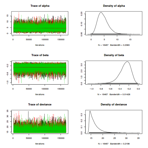
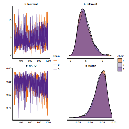
- Lets now explore the chain mixing characteristics
- Trace plots
Show JAGS code
plot(as.mcmc(polis.r2jags))
 Show BRM code
library(gridExtra)
grid.arrange(stan_trace(polis.brm$fit, ncol=1),
             stan_dens(polis.brm$fit, separate_chains=TRUE,ncol=1),
             ncol=2)
- Autocorrelation
Show JAGS code
autocorr.diag(as.mcmc(polis.r2jags))
               alpha        beta     deviance
Lag 0   1.0000000000 1.000000000 1.0000000000
Lag 10  0.3486302850 0.411327730 0.2095816015
Lag 50  0.0077084413 0.015038682 0.0021926870
Lag 100 0.0089742845 0.009909846 0.0009875869
Lag 500 0.0009197652 0.006464200 0.0015197919
## and the centered version
autocorr.diag(as.mcmc(polis.r2jags3))
               alpha         beta    deviance    intercept         LD50    odds_ratio
Lag 0   1.0000000000  1.000000000 1.000000000  1.000000000  1.000000000  1.000000e+00
Lag 10  0.1064366797  0.419052223 0.223137076  0.355734236  0.009911351  3.947151e-01
Lag 50  0.0036116763  0.016284778 0.015703330  0.011656509 -0.001278621  1.288787e-02
Lag 100 0.0041638195  0.001087960 0.005615787  0.001867140  0.002471861  6.922861e-05
Lag 500 0.0007728067 -0.002840246 0.002862181 -0.002974905  0.009877353 -4.708218e-03
Show BRM codeConclusions: there is evidence of autocorrelation (particularly the JAGS model). Note that the samples from the centered models are substantially less uncorrelated. Nevertheless, the JAGS model requires more thinning..stan_ac(polis.brm$fit)
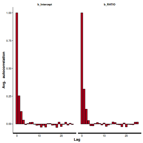
## and the centered version
stan_ac(polis.brm3$fit)
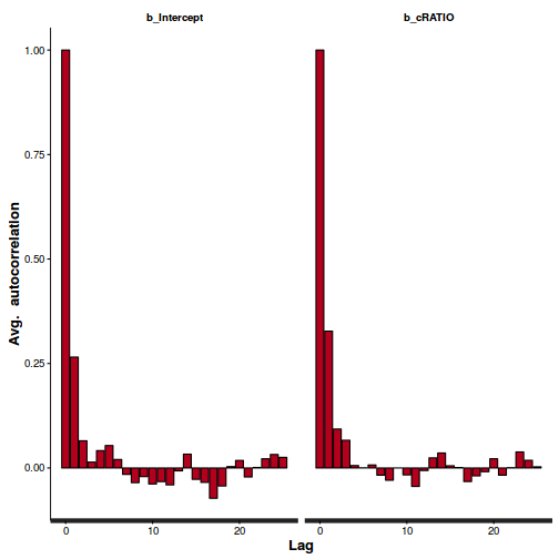 Show the JAGS codeConclusions: that is better..
modelString="
data {
  cratio <- ratio-mean(ratio)
}
model
{
  for (i in 1:n) {
	pa[i] ~ dbern(p[i])
	logit(p[i]) <- alpha+beta*cratio[i]
  }
	alpha~dnorm(0.001,1.0E-6)
	beta ~ dnorm(0.001,1.0E-6)

	#Put the intercept back in the original scale
	intercept <- alpha - beta*mean(ratio)

    #odds ratio
    odds_ratio <- exp(beta)

	#LD50
	LD50<- (-1*intercept)/beta
}
"


polis.list <- with(polis,
                         list(pa=PA,
                         ratio=RATIO,
                         n=nrow(polis))
)


params <- c("alpha","beta", "intercept","odds_ratio","LD50")

adaptSteps = 1000
burnInSteps = 2000
nChains = 3
numSavedSteps = 50000
thinSteps = 10
nIter = ceiling((numSavedSteps * thinSteps)/nChains)

polis.r2jags3 <- jags(data=polis.list,
          inits=NULL,#list(inits,inits,inits), #or inits=list(inits,inits,inits) # since there are three chains
          parameters.to.save=params,
          model.file=textConnection(modelString),
          n.chains=3,
          n.iter=nIter,
          n.burnin=burnInSteps,
      n.thin=100
          )
Compiling data graph
   Resolving undeclared variables
   Allocating nodes
   Initializing
   Reading data back into data table
Compiling model graph
   Resolving undeclared variables
   Allocating nodes
   Graph Size: 128

Initializing model
autocorr.diag(as.mcmc(polis.r2jags3))
                alpha        beta     deviance   intercept        LD50  odds_ratio
Lag 0     1.000000000 1.000000000  1.000000000 1.000000000  1.00000000 1.000000000
Lag 100   0.006012842 0.003251699 -0.001141558 0.009113843  0.01058293 0.006021338
Lag 500  -0.019434918 0.015808090  0.009210730 0.004478822 -0.04252710 0.014713028
Lag 1000  0.021803394 0.015814476 -0.020245532 0.008612682  0.01246592 0.019784439
Lag 5000  0.007324124 0.003770143 -0.007788371 0.014764148  0.01070551 0.005464544
- Step size characteristics (STAN only)
Show BRM code
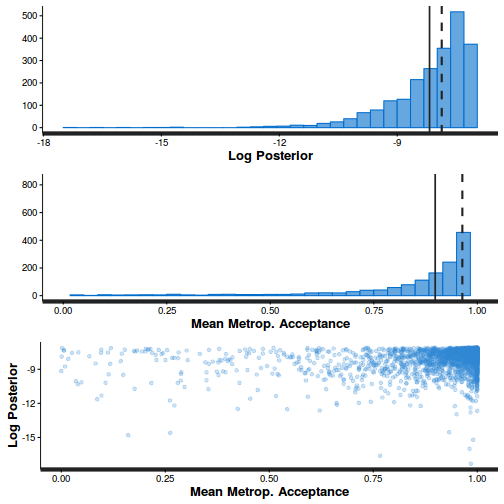
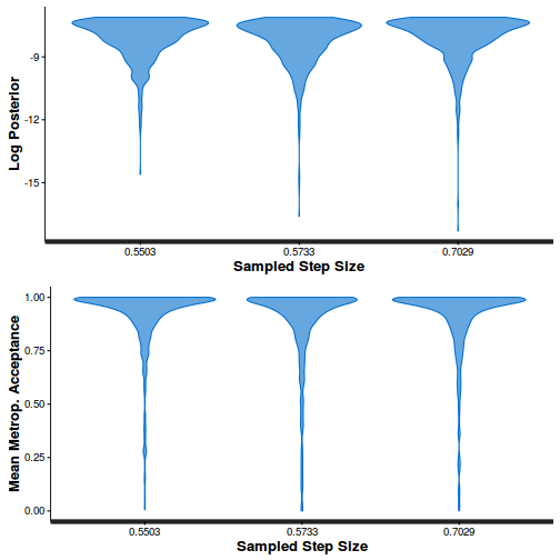
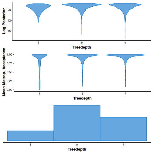
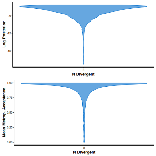
summary(do.call(rbind, args = get_sampler_params(polis.brm3$fit, inc_warmup = FALSE)), digits = 2)
 accept_stat__       stepsize__    treedepth__   n_leapfrog__ n_divergent__
 Min.   :6.1e-05   Min.   :0.55   Min.   :1.0   Min.   :1     Min.   :0
 1st Qu.:8.9e-01   1st Qu.:0.55   1st Qu.:2.0   1st Qu.:3     1st Qu.:0
 Median :9.6e-01   Median :0.57   Median :2.0   Median :3     Median :0
 Mean   :9.0e-01   Mean   :0.61   Mean   :2.2   Mean   :4     Mean   :0
 3rd Qu.:9.9e-01   3rd Qu.:0.70   3rd Qu.:3.0   3rd Qu.:7     3rd Qu.:0
 Max.   :1.0e+00   Max.   :0.70   Max.   :3.0   Max.   :7     Max.   :0
stan_diag(polis.brm3$fit)
stan_diag(polis.brm3$fit, information = "stepsize")
stan_diag(polis.brm3$fit, information = "treedepth")
stan_diag(polis.brm3$fit, information = "divergence")
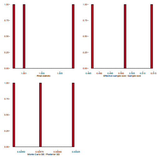
library(gridExtra)
grid.arrange(stan_rhat(polis.brm3$fit) + theme_classic(8),
             stan_ess(polis.brm3$fit) + theme_classic(8),
             stan_mcse(polis.brm3$fit) + theme_classic(8),
             ncol = 2)
- Trace plots
- Now we should check the model fit diagnostics
-
Check the mode for a lack of fit via:
- Check overdispersion
Show JAGS code
#extract the samples for the two model parameters coefs <- polis.r2jags3$BUGSoutput$sims.matrix[,c('alpha','beta')] Xmat <- model.matrix(~x, data=dat) #expected values on a logit scale eta<-coefs %*% t(Xmat) #expected value on response scale pi <- inv.logit(eta) Resid <- -1*sweep(pi,2,polis$PA, '-')/sqrt(pi) RSS <- apply(Resid^2, 1, sum) Disp <- RSS/(nrow(polis)-ncol(coefs)) data.frame(Median=median(Disp), Mean=mean(Disp), HPDinterval(as.mcmc(Disp)), HPDinterval(as.mcmc(Disp),p=0.5))
Median Mean lower upper lower.1 upper.1 var1 49.37055 37914.67 0.2159034 9435.719 0.2159034 49.37055
Show BRM codeResid <- residuals(polis.brm, type='pearson',summary=FALSE) RSS <- apply(Resid^2,1,sum) #sum(Resid[,'Estimate']^2) Disp <- RSS/(nrow(polis)-ncol(coefs)) data.frame(Median=median(Disp), Mean=mean(Disp), HPDinterval(as.mcmc(Disp)))
Median Mean lower upper var1 1.021486 1.077333 0.9623044 1.318911
Show JAGS codeinv.logit <- binomial()$linkinv #Calculate residuals coefs <- polis.r2jags3$BUGSoutput$sims.matrix[,c('alpha','beta')] Xmat <- model.matrix(~cRATIO, data=polis) eta<-coefs %*% t(Xmat) pi <- inv.logit(eta) #sweep across rows and then divide by pi Resid <- -1*sweep(pi,2,polis$PA,'-')/sqrt(pi*(1-pi)) plot(apply(Resid,2,mean)~apply(eta,2,mean)) lines(lowess(apply(Resid,2,mean)~apply(eta,2,mean)))
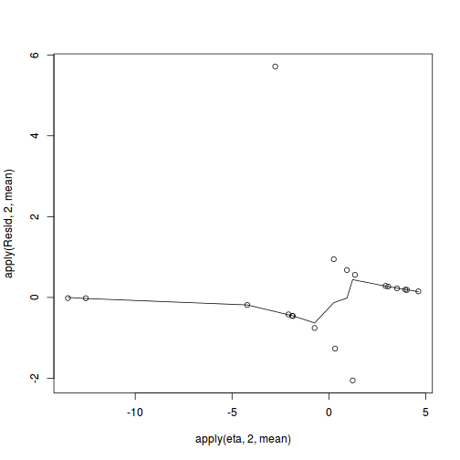
SSres<-apply(Resid^2,1,sum)
set.seed(2)
#generate a matrix of draws from a binomial distribution
# the matrix is the same dimensions as pi and uses the probabilities of pi
YNew <- matrix(rbinom(length(pi),prob=pi,size=1),nrow=nrow(pi))

Resid1<-(pi - YNew)/sqrt(pi*(1-pi))
SSres.sim<-apply(Resid1^2,1,sum)
mean(SSres.sim>SSres)
[1] 0.2493422
Show BRM codeinv.logit <- binomial()$linkinv #Calculate residuals Resid <- residuals(polis.brm3, type='pearson') Fitted <- fitted(polis.brm3, scale='linear') ggplot(data=NULL, aes(y=Resid[,'Estimate'], x=Fitted[,'Estimate'])) + geom_point()
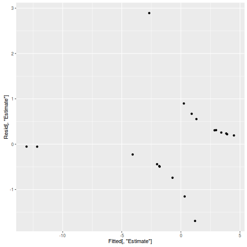
SSres <- sum(Resid[,'Estimate']^2)
pi = fitted(polis.brm3, scale='response')
YNew <- matrix(rbinom(length(pi),prob=pi,size=1),nrow=nrow(pi))

Resid1<-(pi - YNew)/sqrt(pi*(1-pi))
SSres.sim<-apply(Resid1^2,1,sum)
mean(SSres.sim>SSres)
[1] 0
- Check overdispersion
- Explore the parameter estimates
Show JAGS code
print(polis.r2jags3)
Inference for Bugs model at "5", fit using jags,
 3 chains, each with 166667 iterations (first 2000 discarded), n.thin = 100
 n.sims = 4941 iterations saved
           mu.vect sd.vect   2.5%    25%    50%    75%  97.5%  Rhat n.eff
LD50        16.481   3.314 10.612 14.556 16.316 18.239 23.413 1.002  2800
alpha       -0.705   0.855 -2.568 -1.227 -0.645 -0.119  0.801 1.002  1600
beta        -0.288   0.125 -0.588 -0.356 -0.271 -0.196 -0.099 1.002  1400
intercept    4.684   2.090  1.540  3.157  4.410  5.866  9.737 1.002  2400
odds_ratio   0.756   0.090  0.555  0.700  0.762  0.822  0.906 1.002  1400
deviance    16.491   2.243 14.274 14.894 15.803 17.385 22.644 1.002  1900

For each parameter, n.eff is a crude measure of effective sample size,
and Rhat is the potential scale reduction factor (at convergence, Rhat=1).

DIC info (using the rule, pD = var(deviance)/2)
pD = 2.5 and DIC = 19.0
DIC is an estimate of expected predictive error (lower deviance is better).
coefs <- polis.r2jags3$BUGSoutput$sims.matrix[,c('alpha','beta')] plyr:::adply(exp(coefs), 2, function(x) { data.frame(Mean=mean(x), median=median(x), HPDinterval(as.mcmc(x))) } )
     X1      Mean    median       lower     upper
1 alpha 0.6882555 0.5246897 0.007931256 1.8319500
2  beta 0.7558136 0.7623621 0.577557742 0.9232893
Show BRM codeConclusion: Note the 'slope' parameter is on a log odds ratio scale. Typically we would prefer to interpret the model parameters on a natural scale (hence the exponentiated posteriors).print(polis.brm3)
 Family: binomial (logit)
Formula: PA ~ cRATIO
   Data: polis (Number of observations: 19)
Samples: 3 chains, each with iter = 2000; warmup = 500; thin = 2;
         total post-warmup samples = 2250
   WAIC: Not computed

Fixed Effects:
          Estimate Est.Error l-95% CI u-95% CI Eff.Sample Rhat
Intercept    -0.68      0.86    -2.49     0.85       1157    1
cRATIO       -0.28      0.12    -0.55    -0.09       1130    1

Samples were drawn using sampling(NUTS). For each parameter, Eff.Sample
is a crude measure of effective sample size, and Rhat is the potential
scale reduction factor on split chains (at convergence, Rhat = 1).
coefs <- as.matrix(as.data.frame(rstan:::extract(polis.brm3$fit))) coefs <- coefs[,grep('b', colnames(coefs))] plyr:::adply(exp(coefs), 2, function(x) { data.frame(Mean=mean(x), median=median(x), HPDinterval(as.mcmc(x))) })
           X1      Mean    median       lower     upper
1 b_Intercept 0.7094591 0.5522342 0.007441255 1.8576976
2    b_cRATIO 0.7618033 0.7665764 0.598009286 0.9276557
marginal_effects(polis.brm3)
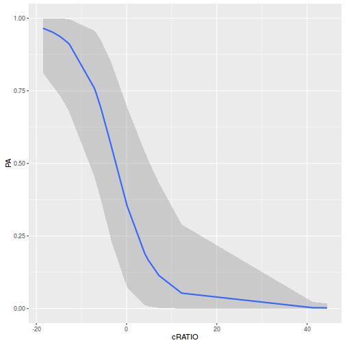
- At the average perimeter to area ratio, the ratio of odds of the lizard being present to the odds of being absent is
0.71 - For each 1 unit increase in perimeter to area ratio, the ratio of odds of being present to odds of being absent changes by a factor of
0.76. Hence, for each 1 unit increase in perimeter, the probability of the lizard being present declines by nearly 25%.
- At the average perimeter to area ratio, the ratio of odds of the lizard being present to the odds of being absent is
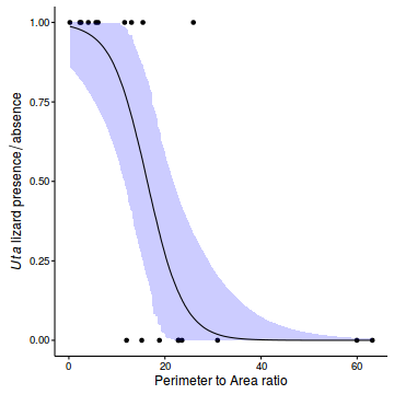
- Construct a scatterplot of the presence/absence of Uta lizards against perimeter to area ratio for the 19 islands
Show JAGS code
newdata <- with(polis, data.frame(cRATIO=seq(min(cRATIO), max(cRATIO), len=1000)))
newdata$RATIO <- newdata$cRATIO+attr(polis$cRATIO, 'mean')
Xmat <- model.matrix(~cRATIO, data=newdata)
coefs <- polis.r2jags3$BUGSoutput$sims.matrix[,c('alpha','beta')]
fit <- inv.logit(coefs %*% t(Xmat))
newdata = cbind(newdata, plyr:::adply(fit, 2, function(x) {
   data.frame(Mean=mean(x), Median=median(x), HPDinterval(as.mcmc(x)))
}))

ggplot(newdata, aes(y=Median, x=RATIO)) +
  geom_point(data=polis, aes(y=PA)) +
  geom_ribbon(aes(ymin=lower, ymax=upper), fill='blue', alpha=0.2) +
  geom_line() +
  scale_x_continuous('Perimeter to Area ratio')+
  scale_y_continuous(expression(italic(Uta)~lizard~presence/absence))+
  theme_classic()+
  theme(axis.line.y=element_line(),axis.line.x=element_line())
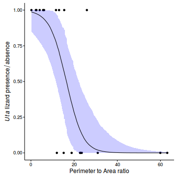
 Show BRM code
newdata <- with(polis, data.frame(cRATIO=seq(min(cRATIO), max(cRATIO), len=1000)))
newdata$RATIO <- newdata$cRATIO+attr(polis$cRATIO, 'mean')
Xmat <- model.matrix(~cRATIO, data=newdata)
coefs <- as.matrix(as.data.frame(rstan:::extract(polis.brm3$fit)))
coefs <- coefs[,grep('b', colnames(coefs))]
fit <- inv.logit(coefs %*% t(Xmat))
newdata = cbind(newdata, plyr:::adply(fit, 2, function(x) {
   data.frame(Mean=mean(x), Median=median(x), HPDinterval(as.mcmc(x)))
}))

ggplot(newdata, aes(y=Median, x=RATIO)) +
  geom_point(data=polis, aes(y=PA)) +
  geom_ribbon(aes(ymin=lower, ymax=upper), fill='blue', alpha=0.2) +
  geom_line() +
  scale_x_continuous('Perimeter to Area ratio')+
  scale_y_continuous(expression(italic(Uta)~lizard~presence/absence))+
  theme_classic()+
  theme(axis.line.y=element_line(),axis.line.x=element_line())
- Calculate the LD50 (in this case, the perimeter to area ratio with a predicted probability of 0.5) from the fitted model
Show JAGS code
coefs <- polis.r2jags3$BUGSoutput$sims.matrix[,c('alpha','beta')]

ld50 <- (-coefs[,1]/coefs[,2]) + attr(polis$cRATIO, 'mean')
data.frame(Mean=mean(ld50), Median=median(ld50),HPDinterval(as.mcmc(ld50)))
        Mean   Median    lower    upper
var1 16.4807 16.31564 10.20908 22.62921
Show BRM codecoefs <- as.matrix(as.data.frame(rstan:::extract(polis.brm3$fit))) coefs <- coefs[,grep('b', colnames(coefs))] ld50 <- (-coefs[,1]/coefs[,2]) + attr(polis$cRATIO, 'mean') data.frame(Mean=mean(ld50), Median=median(ld50),HPDinterval(as.mcmc(ld50)))
         Mean  Median    lower    upper
var1 16.60847 16.4525 10.29575 23.00646
- Calculate the R2 value
Show JAGS code
inv.logit <- binomial()$linkinv
#Calculate residuals
coefs <- polis.r2jags3$BUGSoutput$sims.matrix[,c('alpha','beta')]
Xmat <- model.matrix(~cRATIO, data=polis)
eta<-coefs %*% t(Xmat)
pi <- inv.logit(eta)
#sweep across rows and then divide by pi
Resid <- -1*sweep(pi,2,polis$PA,'-')
R.var <- apply(Resid,1,var)
X.var <- apply(pi,1,var)
R2.marginal <- X.var/(X.var + R.var)
data.frame(Median=median(R2.marginal), coda:::HPDinterval(as.mcmc(R2.marginal)))
        Median     lower     upper
var1 0.5376924 0.3574792 0.6184803
Show BRM codeR.var = apply(residuals(polis.brm3, summary=FALSE),1,var) X.var = apply(fitted(polis.brm3, summary=FALSE),1,var) R2.marginal <- X.var/(X.var + R.var) data.frame(Median=median(R2.marginal), coda:::HPDinterval(as.mcmc(R2.marginal)))
        Median     lower     upper
var1 0.5362865 0.3439372 0.6173302
Proportional data
Arrington et al. (2002) explored patterns in the frequency with which fishes have empty stomachs. In particular, they were interested in investigating whether the frequency of empty stomachs differed between trophic classifications. Live captured fish were classified and the frequency of individuals in each taxa with empty stomachs were tallied.
Download full Arrington data set| Format of arrington_full.csv data file | ||||||||||||||||||||||||||||||||||||||||||||
|---|---|---|---|---|---|---|---|---|---|---|---|---|---|---|---|---|---|---|---|---|---|---|---|---|---|---|---|---|---|---|---|---|---|---|---|---|---|---|---|---|---|---|---|---|
|

|
arrington <- read.csv('../downloads/data/arrington_full.csv', strip.white=T)
head(arrington)
              Order     Family                      Species Location Behaviour     Trophic
1 Osteoglossiformes Mormyridae Hippopotamyrus discorhynchus   Africa Nocturnal Invertivore
2 Osteoglossiformes Mormyridae   Marcusenius macrolepidotus   Africa Nocturnal Invertivore
3 Osteoglossiformes Mormyridae             Mormyrus lacerda   Africa Nocturnal Invertivore
4 Osteoglossiformes Mormyridae      Petrocephalus catostoma   Africa Nocturnal Invertivore
5 Osteoglossiformes Mormyridae        Pollimyrus castelnaui   Africa Nocturnal Invertivore
6     Cypriniformes Cyprinidae             Barbus annectens   Africa   Diurnal    Omnivore
  Individuals Empty Empty_perc
1          37     4 0.10810811
2          83    14 0.16867470
3          46     2 0.04347826
4          11     0 0.00000000
5          47     0 0.00000000
6          17     0 0.00000000
- We might be tempted to fit a simple linear (anova) model to relate frequency (percentage) of empty stomachs
to trophic group. Lets then pursue the regular exploratory data analyses.
Show code
library(ggplot2)
ggplot(arrington, aes(y=Empty_perc, x=Trophic)) + geom_boxplot()
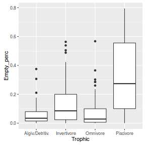
Clearly, these data are not normal and there is some suggestion of a relationship between mean and variance. Furthermore, as there are numerous percentages of zero or close to zero, it is possible that predictions will yield expectations or confidence intervals less than 0.5. This is clearly illogical - it is not possible to have a frequency (percentage) less than zero.
These data present an opportunity to explore a range of analysis options.
- fit a linear model on arcsin transformed percentage of empty stomachs
- fit a linear model on logit transformed percentage of empty stomachs
- fit a generalized linear model (binomial distribution) on frequency (count) of empty stomachs
- Fit a linear model on arcsin transformed percentage of empty stomachs
Show BRM code
#arrington$aEmpty_perc <- asin(sqrt(arrington$Empty_perc))

arrington.brm1 <- brm(asin(sqrt(Empty_perc)) ~ Trophic, data=arrington,
      prior=c(set_prior('normal(0,1000)', class='b'),
              set_prior('cauchy(0,4)', class='sigma')),
      chains=3, iter=2000, warmup=500, thin=2)
SAMPLING FOR MODEL 'gaussian(identity) brms-model' NOW (CHAIN 1).

Chain 1, Iteration:    1 / 2000 [  0%]  (Warmup)
Chain 1, Iteration:  200 / 2000 [ 10%]  (Warmup)
Chain 1, Iteration:  400 / 2000 [ 20%]  (Warmup)
Chain 1, Iteration:  501 / 2000 [ 25%]  (Sampling)
Chain 1, Iteration:  700 / 2000 [ 35%]  (Sampling)
Chain 1, Iteration:  900 / 2000 [ 45%]  (Sampling)
Chain 1, Iteration: 1100 / 2000 [ 55%]  (Sampling)
Chain 1, Iteration: 1300 / 2000 [ 65%]  (Sampling)
Chain 1, Iteration: 1500 / 2000 [ 75%]  (Sampling)
Chain 1, Iteration: 1700 / 2000 [ 85%]  (Sampling)
Chain 1, Iteration: 1900 / 2000 [ 95%]  (Sampling)
Chain 1, Iteration: 2000 / 2000 [100%]  (Sampling)#
#  Elapsed Time: 0.202954 seconds (Warm-up)
#                0.473325 seconds (Sampling)
#                0.676279 seconds (Total)
#

SAMPLING FOR MODEL 'gaussian(identity) brms-model' NOW (CHAIN 2).

Chain 2, Iteration:    1 / 2000 [  0%]  (Warmup)
Chain 2, Iteration:  200 / 2000 [ 10%]  (Warmup)
Chain 2, Iteration:  400 / 2000 [ 20%]  (Warmup)
Chain 2, Iteration:  501 / 2000 [ 25%]  (Sampling)
Chain 2, Iteration:  700 / 2000 [ 35%]  (Sampling)
Chain 2, Iteration:  900 / 2000 [ 45%]  (Sampling)
Chain 2, Iteration: 1100 / 2000 [ 55%]  (Sampling)
Chain 2, Iteration: 1300 / 2000 [ 65%]  (Sampling)
Chain 2, Iteration: 1500 / 2000 [ 75%]  (Sampling)
Chain 2, Iteration: 1700 / 2000 [ 85%]  (Sampling)
Chain 2, Iteration: 1900 / 2000 [ 95%]  (Sampling)
Chain 2, Iteration: 2000 / 2000 [100%]  (Sampling)#
#  Elapsed Time: 0.165517 seconds (Warm-up)
#                0.399017 seconds (Sampling)
#                0.564534 seconds (Total)
#

SAMPLING FOR MODEL 'gaussian(identity) brms-model' NOW (CHAIN 3).

Chain 3, Iteration:    1 / 2000 [  0%]  (Warmup)
Chain 3, Iteration:  200 / 2000 [ 10%]  (Warmup)
Chain 3, Iteration:  400 / 2000 [ 20%]  (Warmup)
Chain 3, Iteration:  501 / 2000 [ 25%]  (Sampling)
Chain 3, Iteration:  700 / 2000 [ 35%]  (Sampling)
Chain 3, Iteration:  900 / 2000 [ 45%]  (Sampling)
Chain 3, Iteration: 1100 / 2000 [ 55%]  (Sampling)
Chain 3, Iteration: 1300 / 2000 [ 65%]  (Sampling)
Chain 3, Iteration: 1500 / 2000 [ 75%]  (Sampling)
Chain 3, Iteration: 1700 / 2000 [ 85%]  (Sampling)
Chain 3, Iteration: 1900 / 2000 [ 95%]  (Sampling)
Chain 3, Iteration: 2000 / 2000 [100%]  (Sampling)#
#  Elapsed Time: 0.165979 seconds (Warm-up)
#                0.455872 seconds (Sampling)
#                0.621851 seconds (Total)
#
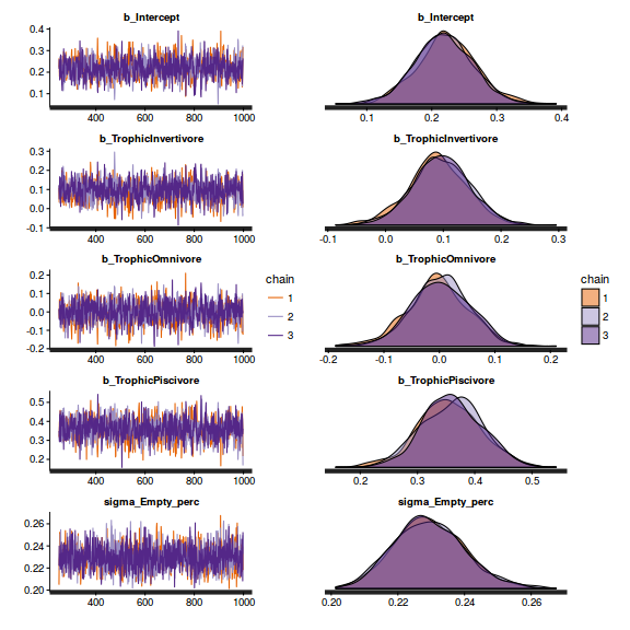
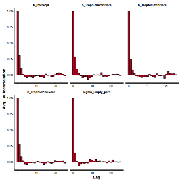
- Check the chain mixing characteristics
Show BRM code for traceplots and autocorrelation
library(gridExtra)
grid.arrange(stan_trace(arrington.brm1$fit, ncol=1),
             stan_dens(arrington.brm1$fit, separate_chains=TRUE,ncol=1),
             ncol=2)
stan_ac(arrington.brm1$fit)
 Show BRM code for step characteristics
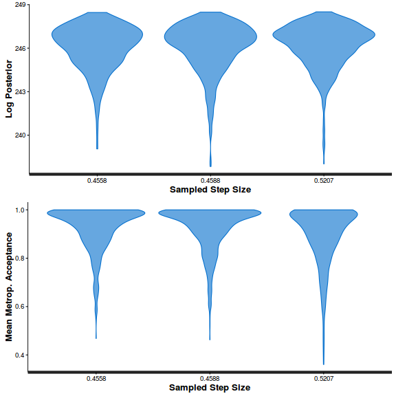
summary(do.call(rbind, args = get_sampler_params(arrington.brm1$fit, inc_warmup = FALSE)), digits = 2)
 accept_stat__    stepsize__    treedepth__   n_leapfrog__  n_divergent__
 Min.   :0.36   Min.   :0.46   Min.   :1.0   Min.   : 1.0   Min.   :0
 1st Qu.:0.87   1st Qu.:0.46   1st Qu.:2.0   1st Qu.: 3.0   1st Qu.:0
 Median :0.95   Median :0.46   Median :3.0   Median : 7.0   Median :0
 Mean   :0.91   Mean   :0.48   Mean   :2.7   Mean   : 6.3   Mean   :0
 3rd Qu.:0.99   3rd Qu.:0.52   3rd Qu.:3.0   3rd Qu.: 7.0   3rd Qu.:0
 Max.   :1.00   Max.   :0.52   Max.   :4.0   Max.   :15.0   Max.   :0
stan_diag(arrington.brm1$fit)
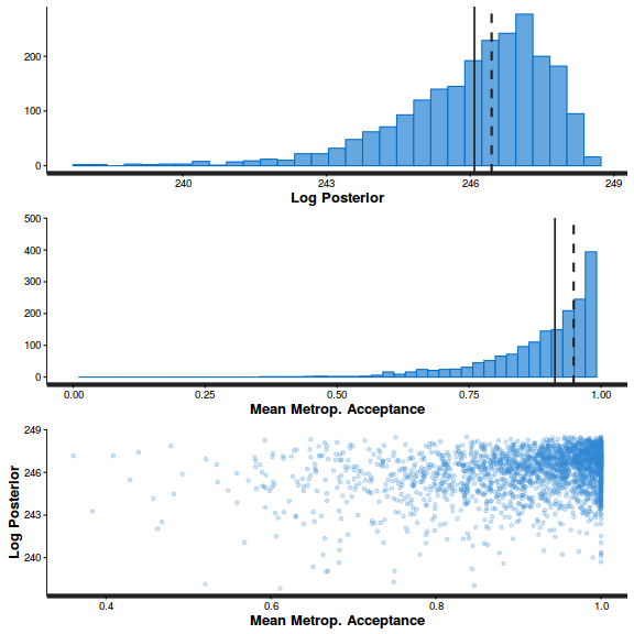
stan_diag(arrington.brm1$fit, information = "stepsize")
library(gridExtra)
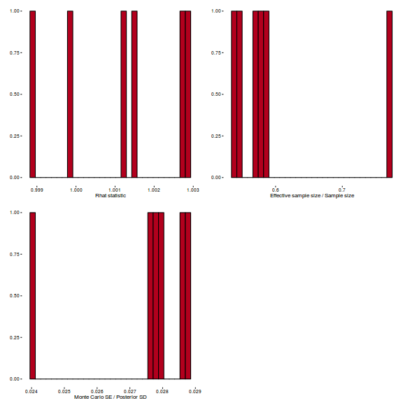
grid.arrange(stan_rhat(arrington.brm1$fit) + theme_classic(8),
             stan_ess(arrington.brm1$fit) + theme_classic(8),
             stan_mcse(arrington.brm1$fit) + theme_classic(8),
             ncol = 2)
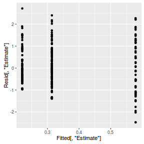
- Check model fit diagnostics
Show BRM code
inv.logit <- binomial()$linkinv
#Calculate residuals
Resid <- residuals(arrington.brm1, type='pearson')
Fitted <- fitted(arrington.brm1, scale='linear')
ggplot(data=NULL, aes(y=Resid[,'Estimate'], x=Fitted[,'Estimate'])) + geom_point()
SSres <- sum(Resid[,'Estimate']^2)
pi = fitted(arrington.brm1, scale='response')
YNew <- matrix(rbinom(length(pi),prob=pi,size=1),nrow=nrow(pi))

Resid1<-(pi - YNew)/sqrt(pi*(1-pi))
SSres.sim<-apply(Resid1^2,1,sum)
mean(SSres.sim>SSres)
[1] 0
## overdispersion
Resid <- residuals(arrington.brm1, type='pearson',summary=FALSE)
RSS <- apply(Resid^2,1,sum) #sum(Resid[,'Estimate']^2)
Disp <- RSS/(nrow(arrington)-ncol(coefs))
data.frame(Median=median(Disp), Mean=mean(Disp), HPDinterval(as.mcmc(Disp)))
        Median      Mean     lower    upper
var1 0.9832764 0.9861594 0.9714418 1.007431
- There are no major concerns with these diagnostics, so we can now explore the model parameters.
Show BRM code
print(arrington.brm1)
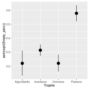
Family: gaussian (identity) Formula: asin(sqrt(Empty_perc)) ~ Trophic Data: arrington (Number of observations: 254) Samples: 3 chains, each with iter = 2000; warmup = 500; thin = 2; total post-warmup samples = 2250 WAIC: Not computed Fixed Effects: Estimate Est.Error l-95% CI u-95% CI Eff.Sample Rhat Intercept 0.22 0.04 0.13 0.31 1208 1 TrophicInvertivore 0.09 0.05 -0.01 0.19 1222 1 TrophicOmnivore 0.00 0.05 -0.11 0.10 1297 1 TrophicPiscivore 0.36 0.05 0.25 0.46 1277 1 Family Specific Parameters: Estimate Est.Error l-95% CI u-95% CI Eff.Sample Rhat sigma(Empty_perc) 0.23 0.01 0.21 0.25 1732 1 Samples were drawn using sampling(NUTS). For each parameter, Eff.Sample is a crude measure of effective sample size, and Rhat is the potential scale reduction factor on split chains (at convergence, Rhat = 1).WAIC(arrington.brm1)
   WAIC    SE
 -23.65 20.66
marginal_effects(arrington.brm1)
- Fit a linear model on arcsin transformed percentage of empty stomachs
Show BRM code
logit <- binomial()$linkfun
logit.inv <- binomial()$linkinv
arrington$Perc <- arrington$Empty_perc + min(arrington$Empty_perc[arrington$Empty_perc>0])
arrington.brm2 <- brm(logit(Perc) ~ Trophic, data=arrington,
      prior=c(set_prior('normal(0,100)', class='b'),
              set_prior('cauchy(0,2)', class='sigma')),
      chains=3, iter=2000, warmup=500, thin=2)
SAMPLING FOR MODEL 'gaussian(identity) brms-model' NOW (CHAIN 1).

Chain 1, Iteration:    1 / 2000 [  0%]  (Warmup)
Chain 1, Iteration:  200 / 2000 [ 10%]  (Warmup)
Chain 1, Iteration:  400 / 2000 [ 20%]  (Warmup)
Chain 1, Iteration:  501 / 2000 [ 25%]  (Sampling)
Chain 1, Iteration:  700 / 2000 [ 35%]  (Sampling)
Chain 1, Iteration:  900 / 2000 [ 45%]  (Sampling)
Chain 1, Iteration: 1100 / 2000 [ 55%]  (Sampling)
Chain 1, Iteration: 1300 / 2000 [ 65%]  (Sampling)
Chain 1, Iteration: 1500 / 2000 [ 75%]  (Sampling)
Chain 1, Iteration: 1700 / 2000 [ 85%]  (Sampling)
Chain 1, Iteration: 1900 / 2000 [ 95%]  (Sampling)
Chain 1, Iteration: 2000 / 2000 [100%]  (Sampling)#
#  Elapsed Time: 0.185868 seconds (Warm-up)
#                0.47553 seconds (Sampling)
#                0.661398 seconds (Total)
#

SAMPLING FOR MODEL 'gaussian(identity) brms-model' NOW (CHAIN 2).

Chain 2, Iteration:    1 / 2000 [  0%]  (Warmup)
Chain 2, Iteration:  200 / 2000 [ 10%]  (Warmup)
Chain 2, Iteration:  400 / 2000 [ 20%]  (Warmup)
Chain 2, Iteration:  501 / 2000 [ 25%]  (Sampling)
Chain 2, Iteration:  700 / 2000 [ 35%]  (Sampling)
Chain 2, Iteration:  900 / 2000 [ 45%]  (Sampling)
Chain 2, Iteration: 1100 / 2000 [ 55%]  (Sampling)
Chain 2, Iteration: 1300 / 2000 [ 65%]  (Sampling)
Chain 2, Iteration: 1500 / 2000 [ 75%]  (Sampling)
Chain 2, Iteration: 1700 / 2000 [ 85%]  (Sampling)
Chain 2, Iteration: 1900 / 2000 [ 95%]  (Sampling)
Chain 2, Iteration: 2000 / 2000 [100%]  (Sampling)#
#  Elapsed Time: 0.202127 seconds (Warm-up)
#                0.438679 seconds (Sampling)
#                0.640806 seconds (Total)
#

SAMPLING FOR MODEL 'gaussian(identity) brms-model' NOW (CHAIN 3).

Chain 3, Iteration:    1 / 2000 [  0%]  (Warmup)
Chain 3, Iteration:  200 / 2000 [ 10%]  (Warmup)
Chain 3, Iteration:  400 / 2000 [ 20%]  (Warmup)
Chain 3, Iteration:  501 / 2000 [ 25%]  (Sampling)
Chain 3, Iteration:  700 / 2000 [ 35%]  (Sampling)
Chain 3, Iteration:  900 / 2000 [ 45%]  (Sampling)
Chain 3, Iteration: 1100 / 2000 [ 55%]  (Sampling)
Chain 3, Iteration: 1300 / 2000 [ 65%]  (Sampling)
Chain 3, Iteration: 1500 / 2000 [ 75%]  (Sampling)
Chain 3, Iteration: 1700 / 2000 [ 85%]  (Sampling)
Chain 3, Iteration: 1900 / 2000 [ 95%]  (Sampling)
Chain 3, Iteration: 2000 / 2000 [100%]  (Sampling)#
#  Elapsed Time: 0.189506 seconds (Warm-up)
#                0.463606 seconds (Sampling)
#                0.653112 seconds (Total)
#
- Check the chain mixing characteristics
Show BRM code for traceplots and autocorrelation
library(gridExtra)
grid.arrange(stan_trace(arrington.brm2$fit, ncol=1),
             stan_dens(arrington.brm2$fit, separate_chains=TRUE,ncol=1),
             ncol=2)
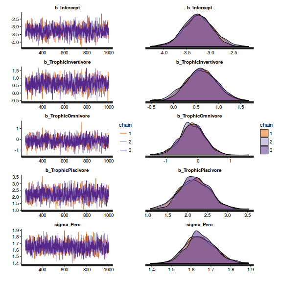
stan_ac(arrington.brm2$fit)
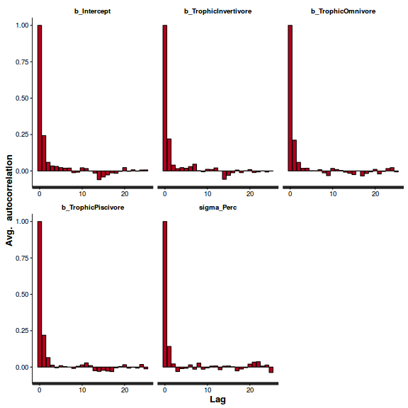 Show BRM code for step characteristics
summary(do.call(rbind, args = get_sampler_params(arrington.brm2$fit, inc_warmup = FALSE)), digits = 2)
 accept_stat__    stepsize__    treedepth__   n_leapfrog__  n_divergent__
 Min.   :0.37   Min.   :0.43   Min.   :1.0   Min.   : 1.0   Min.   :0
 1st Qu.:0.87   1st Qu.:0.43   1st Qu.:2.0   1st Qu.: 3.0   1st Qu.:0
 Median :0.95   Median :0.43   Median :3.0   Median : 7.0   Median :0
 Mean   :0.91   Mean   :0.45   Mean   :2.8   Mean   : 6.5   Mean   :0
 3rd Qu.:0.99   3rd Qu.:0.50   3rd Qu.:3.0   3rd Qu.: 7.0   3rd Qu.:0
 Max.   :1.00   Max.   :0.50   Max.   :4.0   Max.   :15.0   Max.   :0
stan_diag(arrington.brm2$fit)
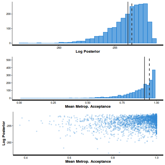
stan_diag(arrington.brm2$fit, information = "stepsize")
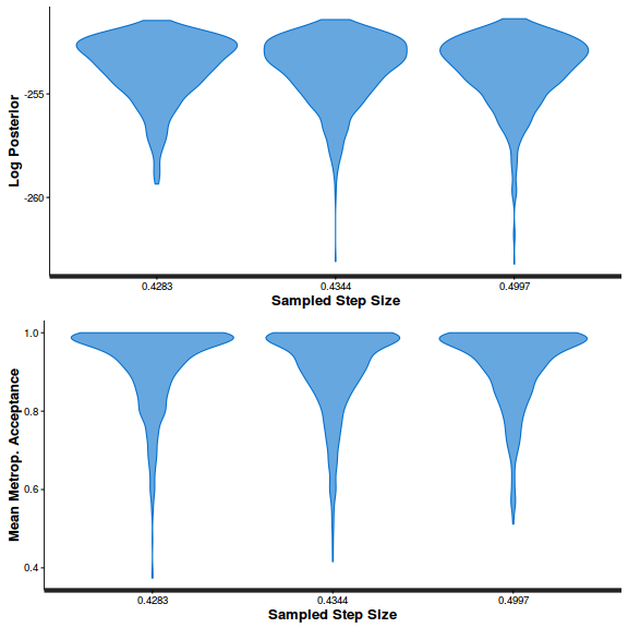
library(gridExtra)
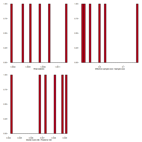
grid.arrange(stan_rhat(arrington.brm2$fit) + theme_classic(8),
             stan_ess(arrington.brm2$fit) + theme_classic(8),
             stan_mcse(arrington.brm2$fit) + theme_classic(8),
             ncol = 2)
- Check model fit diagnostics
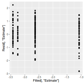
Show BRM code
inv.logit <- binomial()$linkinv
#Calculate residuals
Resid <- residuals(arrington.brm2, type='pearson')
Fitted <- fitted(arrington.brm2, scale='linear')
ggplot(data=NULL, aes(y=Resid[,'Estimate'], x=Fitted[,'Estimate'])) + geom_point()
SSres <- sum(Resid[,'Estimate']^2)
pi = fitted(arrington.brm2, scale='response')
YNew <- matrix(rbinom(length(pi),prob=pi,size=1),nrow=nrow(pi))

Resid1<-(pi - YNew)/sqrt(pi*(1-pi))
SSres.sim<-apply(Resid1^2,1,sum)
mean(SSres.sim>SSres)
[1] NA
## overdispersion
Resid <- residuals(arrington.brm2, type='pearson',summary=FALSE)
RSS <- apply(Resid^2,1,sum) #sum(Resid[,'Estimate']^2)
Disp <- RSS/(nrow(arrington)-ncol(coefs))
data.frame(Median=median(Disp), Mean=mean(Disp), HPDinterval(as.mcmc(Disp)))
        Median      Mean     lower    upper
var1 0.9881678 0.9906284 0.9756028 1.011514
- There are no major concerns with these diagnostics, so we can now explore the model parameters.
Show BRM code
print(arrington.brm2)
Family: gaussian (identity) Formula: logit(Perc) ~ Trophic Data: arrington (Number of observations: 254) Samples: 3 chains, each with iter = 2000; warmup = 500; thin = 2; total post-warmup samples = 2250 WAIC: Not computed Fixed Effects: Estimate Est.Error l-95% CI u-95% CI Eff.Sample Rhat Intercept -3.25 0.31 -3.86 -2.64 1183 1 TrophicInvertivore 0.62 0.35 -0.04 1.30 1213 1 TrophicOmnivore -0.17 0.38 -0.94 0.58 1341 1 TrophicPiscivore 2.18 0.38 1.46 2.94 1397 1 Family Specific Parameters: Estimate Est.Error l-95% CI u-95% CI Eff.Sample Rhat sigma(Perc) 1.65 0.07 1.51 1.81 1704 1 Samples were drawn using sampling(NUTS). For each parameter, Eff.Sample is a crude measure of effective sample size, and Rhat is the potential scale reduction factor on split chains (at convergence, Rhat = 1).WAIC(arrington.brm2)
   WAIC    SE
 979.13 20.75
marginal_effects(arrington.brm2)
Error in logit(Perc): REAL() can only be applied to a 'numeric', not a 'logical'
- Rather than transform the raw data in order to satisfy the requirements of linear regression,
it is arguably better to fir a model that is more appropriate for the response variable. In this case, since
the response is the frequency (proportion) of empty stomachs from a set of fish, we could argue that this is a
good match for a binomial distribution. Proportions are bound to the range [0,1] and we might expect a certain
degree of relationship between location and scale (mean and variance).
The glm() function allows us to work with either proportions or frequencies (the actual counts), so in the following, we will fit the model both ways. These can be considered as identical alternatives.
Show codearrington.brm3 <- brm(Empty|trials(Individuals) ~ Trophic, data=arrington, family=binomial, prior=c(set_prior('normal(0,100)', class='b')), chains=3, iter=2000, warmup=500, thin=2)
SAMPLING FOR MODEL 'binomial(logit) brms-model' NOW (CHAIN 1).

Chain 1, Iteration:    1 / 2000 [  0%]  (Warmup)
Chain 1, Iteration:  200 / 2000 [ 10%]  (Warmup)
Chain 1, Iteration:  400 / 2000 [ 20%]  (Warmup)
Chain 1, Iteration:  501 / 2000 [ 25%]  (Sampling)
Chain 1, Iteration:  700 / 2000 [ 35%]  (Sampling)
Chain 1, Iteration:  900 / 2000 [ 45%]  (Sampling)
Chain 1, Iteration: 1100 / 2000 [ 55%]  (Sampling)
Chain 1, Iteration: 1300 / 2000 [ 65%]  (Sampling)
Chain 1, Iteration: 1500 / 2000 [ 75%]  (Sampling)
Chain 1, Iteration: 1700 / 2000 [ 85%]  (Sampling)
Chain 1, Iteration: 1900 / 2000 [ 95%]  (Sampling)
Chain 1, Iteration: 2000 / 2000 [100%]  (Sampling)#
#  Elapsed Time: 0.387319 seconds (Warm-up)
#                1.1419 seconds (Sampling)
#                1.52921 seconds (Total)
#

SAMPLING FOR MODEL 'binomial(logit) brms-model' NOW (CHAIN 2).

Chain 2, Iteration:    1 / 2000 [  0%]  (Warmup)
Chain 2, Iteration:  200 / 2000 [ 10%]  (Warmup)
Chain 2, Iteration:  400 / 2000 [ 20%]  (Warmup)
Chain 2, Iteration:  501 / 2000 [ 25%]  (Sampling)
Chain 2, Iteration:  700 / 2000 [ 35%]  (Sampling)
Chain 2, Iteration:  900 / 2000 [ 45%]  (Sampling)
Chain 2, Iteration: 1100 / 2000 [ 55%]  (Sampling)
Chain 2, Iteration: 1300 / 2000 [ 65%]  (Sampling)
Chain 2, Iteration: 1500 / 2000 [ 75%]  (Sampling)
Chain 2, Iteration: 1700 / 2000 [ 85%]  (Sampling)
Chain 2, Iteration: 1900 / 2000 [ 95%]  (Sampling)
Chain 2, Iteration: 2000 / 2000 [100%]  (Sampling)#
#  Elapsed Time: 0.374409 seconds (Warm-up)
#                1.05255 seconds (Sampling)
#                1.42696 seconds (Total)
#

SAMPLING FOR MODEL 'binomial(logit) brms-model' NOW (CHAIN 3).

Chain 3, Iteration:    1 / 2000 [  0%]  (Warmup)
Chain 3, Iteration:  200 / 2000 [ 10%]  (Warmup)
Chain 3, Iteration:  400 / 2000 [ 20%]  (Warmup)
Chain 3, Iteration:  501 / 2000 [ 25%]  (Sampling)
Chain 3, Iteration:  700 / 2000 [ 35%]  (Sampling)
Chain 3, Iteration:  900 / 2000 [ 45%]  (Sampling)
Chain 3, Iteration: 1100 / 2000 [ 55%]  (Sampling)
Chain 3, Iteration: 1300 / 2000 [ 65%]  (Sampling)
Chain 3, Iteration: 1500 / 2000 [ 75%]  (Sampling)
Chain 3, Iteration: 1700 / 2000 [ 85%]  (Sampling)
Chain 3, Iteration: 1900 / 2000 [ 95%]  (Sampling)
Chain 3, Iteration: 2000 / 2000 [100%]  (Sampling)#
#  Elapsed Time: 0.387403 seconds (Warm-up)
#                0.965986 seconds (Sampling)
#                1.35339 seconds (Total)
#
- Check the chain mixing characteristics
Show BRM code for traceplots and autocorrelation
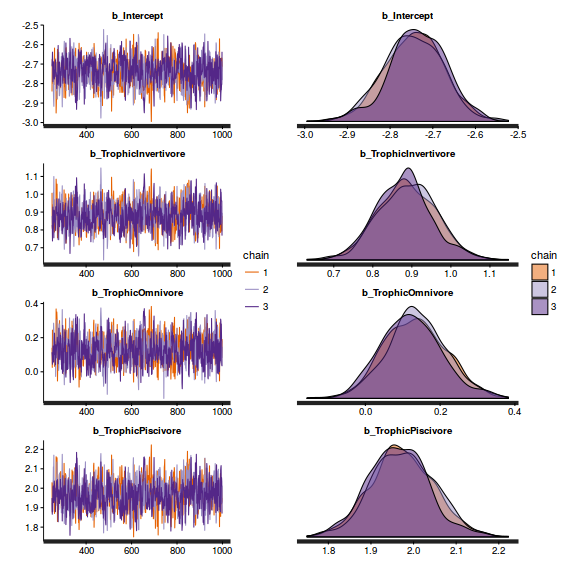
library(gridExtra)
grid.arrange(stan_trace(arrington.brm3$fit, ncol=1),
             stan_dens(arrington.brm3$fit, separate_chains=TRUE,ncol=1),
             ncol=2)
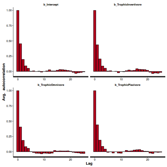
stan_ac(arrington.brm3$fit)
 Show BRM code for step characteristics
summary(do.call(rbind, args = get_sampler_params(arrington.brm3$fit, inc_warmup = FALSE)), digits = 2)
 accept_stat__    stepsize__    treedepth__  n_leapfrog__  n_divergent__
 Min.   :0.37   Min.   :0.29   Min.   :1    Min.   : 1.0   Min.   :0
 1st Qu.:0.90   1st Qu.:0.29   1st Qu.:2    1st Qu.: 3.0   1st Qu.:0
 Median :0.96   Median :0.33   Median :3    Median : 7.0   Median :0
 Mean   :0.93   Mean   :0.33   Mean   :3    Mean   : 7.9   Mean   :0
 3rd Qu.:0.99   3rd Qu.:0.38   3rd Qu.:4    3rd Qu.:11.0   3rd Qu.:0
 Max.   :1.00   Max.   :0.38   Max.   :5    Max.   :31.0   Max.   :0
stan_diag(arrington.brm3$fit)
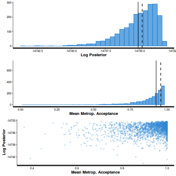
stan_diag(arrington.brm3$fit, information = "stepsize")
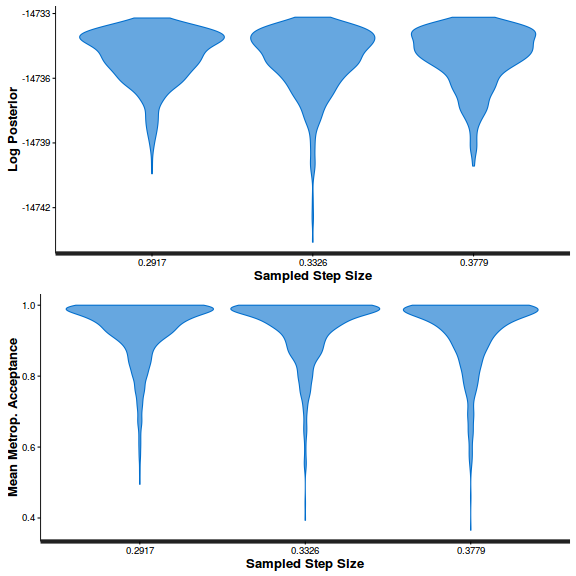
library(gridExtra)
grid.arrange(stan_rhat(arrington.brm3$fit) + theme_classic(8),
             stan_ess(arrington.brm3$fit) + theme_classic(8),
             stan_mcse(arrington.brm3$fit) + theme_classic(8),
             ncol = 2)
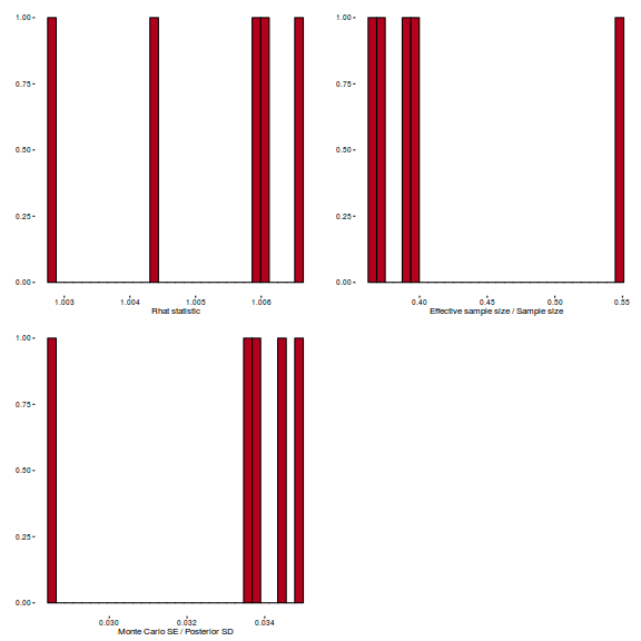
- Check model fit diagnostics
Show BRM code
inv.logit <- binomial()$linkinv
#Calculate residuals
Resid <- residuals(arrington.brm3, type='pearson')
Fitted <- fitted(arrington.brm3, scale='linear')
ggplot(data=NULL, aes(y=Resid[,'Estimate'], x=Fitted[,'Estimate'])) + geom_point()
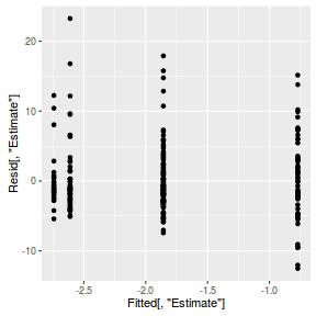
SSres <- sum(Resid[,'Estimate']^2)
pi = fitted(arrington.brm3, scale='response')
YNew <- matrix(rbinom(length(pi),prob=pi,size=1),nrow=nrow(pi))

Resid1<-(pi - YNew)/sqrt(pi*(1-pi))
SSres.sim<-apply(Resid1^2,1,sum)
mean(SSres.sim>SSres)
[1] NA
## overdispersion
Resid <- residuals(arrington.brm3, type='pearson',summary=FALSE)
RSS <- apply(Resid^2,1,sum) #sum(Resid[,'Estimate']^2)
Disp <- RSS/(nrow(arrington)-ncol(coefs))
data.frame(Median=median(Disp), Mean=mean(Disp), HPDinterval(as.mcmc(Disp)))
       Median     Mean    lower    upper
var1 24.51102 24.51353 24.49827 24.53387
- There are no major concerns with these diagnostics, so we can now explore the model parameters.
Show BRM code
print(arrington.brm3)
Family: binomial (logit) Formula: Empty | trials(Individuals) ~ Trophic Data: arrington (Number of observations: 254) Samples: 3 chains, each with iter = 2000; warmup = 500; thin = 2; total post-warmup samples = 2250 WAIC: Not computed Fixed Effects: Estimate Est.Error l-95% CI u-95% CI Eff.Sample Rhat Intercept -2.74 0.07 -2.88 -2.61 826 1.01 TrophicInvertivore 0.89 0.07 0.75 1.03 841 1.01 TrophicOmnivore 0.13 0.08 -0.02 0.30 888 1.00 TrophicPiscivore 1.97 0.07 1.83 2.12 876 1.01 Samples were drawn using sampling(NUTS). For each parameter, Eff.Sample is a crude measure of effective sample size, and Rhat is the potential scale reduction factor on split chains (at convergence, Rhat = 1).WAIC(arrington.brm3)
    WAIC     SE
 6915.29 682.35
- The model is clearly overdispersed... There are numerous ways of addressing this:
- overdispersion is often the result of the model failing to adequately capturing the full variability in the data. Data might be more variable than expected by a model (and its distribution) because of latent effects (additional influences that are not measured or incorporated in the model). If so, then adding a unit (or observation) level random effect (a latent variable) can address overdispersion by soaking up the additional variability. In this relatively simple example, a unit level random effect is simply a variable with the numbers 1 through to the number of rows in the data. Hence, each observation has a unique value (level). In more complex examples, it might be necessary to nest the number sequence within blocks.
- fit a model against a distribution that does not assume dispersion is 1 and has an ability to estimate both location and scale (such as a beta-binomial.
- Lets first try fitting an observation-level random effect in a hierarchical generalized linear model
Show BRM code
arrington$Obs <- 1:nrow(arrington)
arrington.brm4 <- brm(Empty|trials(Individuals) ~ Trophic +(1|Obs), data=arrington, family=binomial,
       prior=c(set_prior('normal(0,100)', class='b'),
               set_prior('cauchy(0,2)', class='sd')),
       chains=3, iter=2000, warmup=500, thin=10)
SAMPLING FOR MODEL 'binomial(logit) brms-model' NOW (CHAIN 1).

Chain 1, Iteration:    1 / 2000 [  0%]  (Warmup)
Chain 1, Iteration:  200 / 2000 [ 10%]  (Warmup)
Chain 1, Iteration:  400 / 2000 [ 20%]  (Warmup)
Chain 1, Iteration:  501 / 2000 [ 25%]  (Sampling)
Chain 1, Iteration:  700 / 2000 [ 35%]  (Sampling)
Chain 1, Iteration:  900 / 2000 [ 45%]  (Sampling)
Chain 1, Iteration: 1100 / 2000 [ 55%]  (Sampling)
Chain 1, Iteration: 1300 / 2000 [ 65%]  (Sampling)
Chain 1, Iteration: 1500 / 2000 [ 75%]  (Sampling)
Chain 1, Iteration: 1700 / 2000 [ 85%]  (Sampling)
Chain 1, Iteration: 1900 / 2000 [ 95%]  (Sampling)
Chain 1, Iteration: 2000 / 2000 [100%]  (Sampling)#
#  Elapsed Time: 4.52238 seconds (Warm-up)
#                9.73738 seconds (Sampling)
#                14.2598 seconds (Total)
#

SAMPLING FOR MODEL 'binomial(logit) brms-model' NOW (CHAIN 2).

Chain 2, Iteration:    1 / 2000 [  0%]  (Warmup)
Chain 2, Iteration:  200 / 2000 [ 10%]  (Warmup)
Chain 2, Iteration:  400 / 2000 [ 20%]  (Warmup)
Chain 2, Iteration:  501 / 2000 [ 25%]  (Sampling)
Chain 2, Iteration:  700 / 2000 [ 35%]  (Sampling)
Chain 2, Iteration:  900 / 2000 [ 45%]  (Sampling)
Chain 2, Iteration: 1100 / 2000 [ 55%]  (Sampling)
Chain 2, Iteration: 1300 / 2000 [ 65%]  (Sampling)
Chain 2, Iteration: 1500 / 2000 [ 75%]  (Sampling)
Chain 2, Iteration: 1700 / 2000 [ 85%]  (Sampling)
Chain 2, Iteration: 1900 / 2000 [ 95%]  (Sampling)
Chain 2, Iteration: 2000 / 2000 [100%]  (Sampling)#
#  Elapsed Time: 4.65143 seconds (Warm-up)
#                9.25017 seconds (Sampling)
#                13.9016 seconds (Total)
#

SAMPLING FOR MODEL 'binomial(logit) brms-model' NOW (CHAIN 3).

Chain 3, Iteration:    1 / 2000 [  0%]  (Warmup)
Chain 3, Iteration:  200 / 2000 [ 10%]  (Warmup)
Chain 3, Iteration:  400 / 2000 [ 20%]  (Warmup)
Chain 3, Iteration:  501 / 2000 [ 25%]  (Sampling)
Chain 3, Iteration:  700 / 2000 [ 35%]  (Sampling)
Chain 3, Iteration:  900 / 2000 [ 45%]  (Sampling)
Chain 3, Iteration: 1100 / 2000 [ 55%]  (Sampling)
Chain 3, Iteration: 1300 / 2000 [ 65%]  (Sampling)
Chain 3, Iteration: 1500 / 2000 [ 75%]  (Sampling)
Chain 3, Iteration: 1700 / 2000 [ 85%]  (Sampling)
Chain 3, Iteration: 1900 / 2000 [ 95%]  (Sampling)
Chain 3, Iteration: 2000 / 2000 [100%]  (Sampling)#
#  Elapsed Time: 4.40266 seconds (Warm-up)
#                9.61914 seconds (Sampling)
#                14.0218 seconds (Total)
#
- Check the chain mixing characteristics
Show BRM code for traceplots and autocorrelation
library(gridExtra)
grid.arrange(stan_trace(arrington.brm4$fit, ncol=1),
             stan_dens(arrington.brm4$fit, separate_chains=TRUE,ncol=1),
             ncol=2)
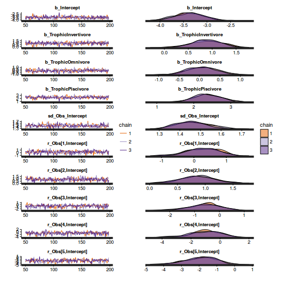
stan_ac(arrington.brm4$fit)
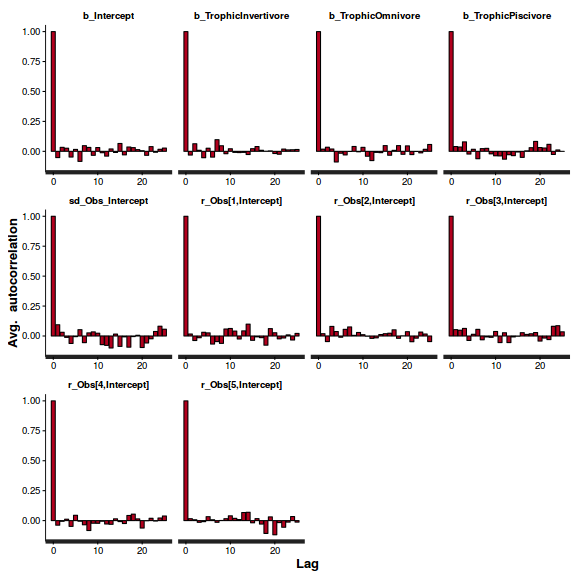 Show BRM code for step characteristics
summary(do.call(rbind, args = get_sampler_params(arrington.brm4$fit, inc_warmup = FALSE)), digits = 2)
 accept_stat__    stepsize__     treedepth__  n_leapfrog__ n_divergent__
 Min.   :0.52   Min.   :0.072   Min.   :5    Min.   :31    Min.   :0
 1st Qu.:0.89   1st Qu.:0.072   1st Qu.:6    1st Qu.:63    1st Qu.:0
 Median :0.95   Median :0.074   Median :6    Median :63    Median :0
 Mean   :0.92   Mean   :0.075   Mean   :6    Mean   :62    Mean   :0
 3rd Qu.:0.98   3rd Qu.:0.080   3rd Qu.:6    3rd Qu.:63    3rd Qu.:0
 Max.   :1.00   Max.   :0.080   Max.   :6    Max.   :63    Max.   :0
stan_diag(arrington.brm4$fit)
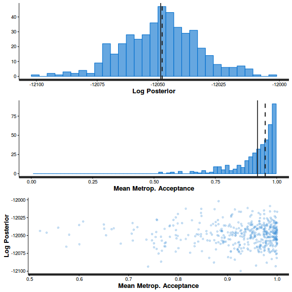
stan_diag(arrington.brm4$fit, information = "stepsize")
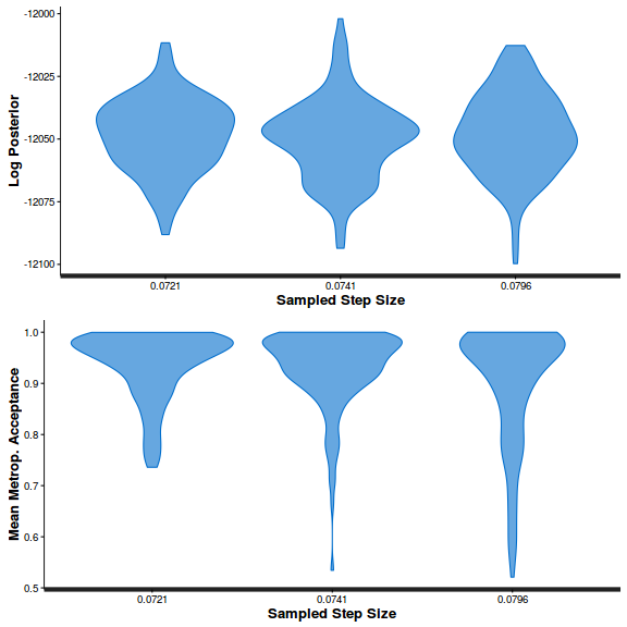
library(gridExtra)
grid.arrange(stan_rhat(arrington.brm4$fit) + theme_classic(8),
             stan_ess(arrington.brm4$fit) + theme_classic(8),
             stan_mcse(arrington.brm4$fit) + theme_classic(8),
             ncol = 2)
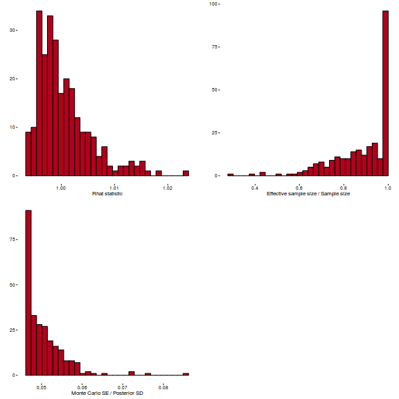
- Check model fit diagnostics
Show BRM code
## rather than explore residuals plots, we should plot the random effects against the
## predicted values from the fixed effect component of the model and check for no trend:
ran = ranef(arrington.brm4)$Obs
Xmat = model.matrix(~Trophic, data=arrington)
fit = Xmat%*%fixef(arrington.brm4)
ggplot(data=NULL, aes(y=ran, x=fit)) + geom_point()
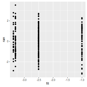
## looks good..


## overdispersion
Resid <- residuals(arrington.brm4, type='pearson',summary=FALSE)
RSS <- apply(Resid^2,1,sum) #sum(Resid[,'Estimate']^2)
Disp <- RSS/(nrow(arrington)-ncol(coefs))
data.frame(Median=median(Disp), Mean=mean(Disp), HPDinterval(as.mcmc(Disp)))
        Median      Mean     lower     upper
var1 0.5608449 0.5629726 0.4400656 0.6863668
- There are no major concerns with these diagnostics, so we can now explore the model parameters.
Show BRM code
print(arrington.brm4)
Family: binomial (logit) Formula: Empty | trials(Individuals) ~ Trophic + (1 | Obs) Data: arrington (Number of observations: 254) Samples: 3 chains, each with iter = 2000; warmup = 500; thin = 10; total post-warmup samples = 450 WAIC: Not computed Random Effects: ~Obs (Number of levels: 254) Estimate Est.Error l-95% CI u-95% CI Eff.Sample Rhat sd(Intercept) 1.46 0.08 1.32 1.64 363 1 Fixed Effects: Estimate Est.Error l-95% CI u-95% CI Eff.Sample Rhat Intercept -3.38 0.32 -3.94 -2.78 450 1.00 TrophicInvertivore 0.87 0.34 0.16 1.51 450 0.99 TrophicOmnivore 0.07 0.38 -0.69 0.82 375 1.01 TrophicPiscivore 2.38 0.37 1.65 3.12 334 1.00 Samples were drawn using sampling(NUTS). For each parameter, Eff.Sample is a crude measure of effective sample size, and Rhat is the potential scale reduction factor on split chains (at convergence, Rhat = 1).WAIC(arrington.brm4)
    WAIC    SE
 1279.27 27.91
- Definitely worth a summary figure.
Show BRM code
newdata = data.frame(Trophic = levels(arrington$Trophic))
Xmat <- model.matrix(~Trophic, data=newdata)
coefs <- as.matrix(as.data.frame(rstan:::extract(arrington.brm4$fit)))
coefs <- coefs[,grep('^b_', colnames(coefs))]
inv.logit <- binomial()$linkinv
fit = inv.logit(coefs %*% t(Xmat))
newdata = cbind(newdata, plyr:::adply(fit, 2, function(x) {
   data.frame(Mean=mean(x), Median=median(x), HPDinterval(as.mcmc(x)))
}))

ggplot(newdata, aes(y=Median, x=Trophic)) +
  geom_blank()+
  geom_pointrange(aes(ymin=lower, ymax=upper, x=as.numeric(Trophic))) +
  scale_y_continuous('Proportion of individuals with empty stomachs')+
  scale_x_discrete('Trophic Group')+
  theme_classic() +
  theme(axis.line.x=element_line(),axis.line.y=element_line(),
        axis.title.x=element_text(margin=margin(t=2, unit='lines')),
        axis.title.y=element_text(margin=margin(r=2, unit='lines')))
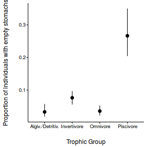
- Give it a go...
Show BRM code
arrington.brm4 <- brm(Empty|trials(Individuals) ~ Trophic, data=arrington, family=binomial,
       prior=c(set_prior('normal(0,100)', class='b')),
       chains=3, iter=2000, warmup=500, thin=2)
SAMPLING FOR MODEL 'binomial(logit) brms-model' NOW (CHAIN 1).

Chain 1, Iteration:    1 / 2000 [  0%]  (Warmup)
Chain 1, Iteration:  200 / 2000 [ 10%]  (Warmup)
Chain 1, Iteration:  400 / 2000 [ 20%]  (Warmup)
Chain 1, Iteration:  501 / 2000 [ 25%]  (Sampling)
Chain 1, Iteration:  700 / 2000 [ 35%]  (Sampling)
Chain 1, Iteration:  900 / 2000 [ 45%]  (Sampling)
Chain 1, Iteration: 1100 / 2000 [ 55%]  (Sampling)
Chain 1, Iteration: 1300 / 2000 [ 65%]  (Sampling)
Chain 1, Iteration: 1500 / 2000 [ 75%]  (Sampling)
Chain 1, Iteration: 1700 / 2000 [ 85%]  (Sampling)
Chain 1, Iteration: 1900 / 2000 [ 95%]  (Sampling)
Chain 1, Iteration: 2000 / 2000 [100%]  (Sampling)#
#  Elapsed Time: 0.395135 seconds (Warm-up)
#                1.12591 seconds (Sampling)
#                1.52105 seconds (Total)
#

SAMPLING FOR MODEL 'binomial(logit) brms-model' NOW (CHAIN 2).

Chain 2, Iteration:    1 / 2000 [  0%]  (Warmup)
Chain 2, Iteration:  200 / 2000 [ 10%]  (Warmup)
Chain 2, Iteration:  400 / 2000 [ 20%]  (Warmup)
Chain 2, Iteration:  501 / 2000 [ 25%]  (Sampling)
Chain 2, Iteration:  700 / 2000 [ 35%]  (Sampling)
Chain 2, Iteration:  900 / 2000 [ 45%]  (Sampling)
Chain 2, Iteration: 1100 / 2000 [ 55%]  (Sampling)
Chain 2, Iteration: 1300 / 2000 [ 65%]  (Sampling)
Chain 2, Iteration: 1500 / 2000 [ 75%]  (Sampling)
Chain 2, Iteration: 1700 / 2000 [ 85%]  (Sampling)
Chain 2, Iteration: 1900 / 2000 [ 95%]  (Sampling)
Chain 2, Iteration: 2000 / 2000 [100%]  (Sampling)#
#  Elapsed Time: 0.365576 seconds (Warm-up)
#                1.10701 seconds (Sampling)
#                1.47258 seconds (Total)
#

SAMPLING FOR MODEL 'binomial(logit) brms-model' NOW (CHAIN 3).

Chain 3, Iteration:    1 / 2000 [  0%]  (Warmup)
Chain 3, Iteration:  200 / 2000 [ 10%]  (Warmup)
Chain 3, Iteration:  400 / 2000 [ 20%]  (Warmup)
Chain 3, Iteration:  501 / 2000 [ 25%]  (Sampling)
Chain 3, Iteration:  700 / 2000 [ 35%]  (Sampling)
Chain 3, Iteration:  900 / 2000 [ 45%]  (Sampling)
Chain 3, Iteration: 1100 / 2000 [ 55%]  (Sampling)
Chain 3, Iteration: 1300 / 2000 [ 65%]  (Sampling)
Chain 3, Iteration: 1500 / 2000 [ 75%]  (Sampling)
Chain 3, Iteration: 1700 / 2000 [ 85%]  (Sampling)
Chain 3, Iteration: 1900 / 2000 [ 95%]  (Sampling)
Chain 3, Iteration: 2000 / 2000 [100%]  (Sampling)#
#  Elapsed Time: 0.382143 seconds (Warm-up)
#                0.926586 seconds (Sampling)
#                1.30873 seconds (Total)
#
stancode(arrington.brm4)
functions { } data { int<lower=1> N; // number of observations int Y[N]; // response variable int<lower=1> K; // number of fixed effects matrix[N, K] X; // FE design matrix vector[K] X_means; // column means of X int trials[N]; // number of trials } transformed data { } parameters { real temp_Intercept; // temporary Intercept vector[K] b; // fixed effects } transformed parameters { vector[N] eta; // linear predictor // compute linear predictor eta <- X * b + temp_Intercept; } model { // prior specifications b ~ normal(0,100); // likelihood contribution Y ~ binomial_logit(trials, eta); } generated quantities { real b_Intercept; // fixed effects intercept b_Intercept <- temp_Intercept - dot_product(X_means, b); }modelString=" data { int<lower=1> N; // number of observations int Y[N]; // response variable int<lower=1> K; // number of fixed effects matrix[N, K] X; // FE design matrix vector[K] X_means; // column means of X int trials[N]; // number of trials } transformed data { } parameters { vector[K] b; // fixed effects real intercept; real phi; //overdispersion parameter } transformed parameters { vector[N] eta; // linear predictor vector[N] alpha; //first shape parameter vector[N] beta; //second shape parameter // compute linear predictor for (i in 1:N) eta[i] <- inv_logit(X[i,] * b + intercept); alpha <- eta*phi; beta <- (1-eta)*phi; } model { // prior specifications intercept ~ normal(0,100); b ~ normal(0,100); // likelihood contribution Y ~ beta_binomial(trials, alpha,beta); } generated quantities { } " library(rstan) arrington.rstan <- stan(data=standata(arrington.brm4), model_code=modelString, chains=3, iter=1000, warmup=500, thin=2, save_dso=TRUE )
SAMPLING FOR MODEL '0f53c5d078293f511e328ffcf4d8078a' NOW (CHAIN 1).

Chain 1, Iteration:   1 / 1000 [  0%]  (Warmup)
Chain 1, Iteration: 100 / 1000 [ 10%]  (Warmup)
Chain 1, Iteration: 200 / 1000 [ 20%]  (Warmup)
Chain 1, Iteration: 300 / 1000 [ 30%]  (Warmup)
Chain 1, Iteration: 400 / 1000 [ 40%]  (Warmup)
Chain 1, Iteration: 500 / 1000 [ 50%]  (Warmup)
Chain 1, Iteration: 501 / 1000 [ 50%]  (Sampling)
Chain 1, Iteration: 600 / 1000 [ 60%]  (Sampling)
Chain 1, Iteration: 700 / 1000 [ 70%]  (Sampling)
Chain 1, Iteration: 800 / 1000 [ 80%]  (Sampling)
Chain 1, Iteration: 900 / 1000 [ 90%]  (Sampling)
Chain 1, Iteration: 1000 / 1000 [100%]  (Sampling)#
#  Elapsed Time: 407.543 seconds (Warm-up)
#                404.442 seconds (Sampling)
#                811.985 seconds (Total)
#

SAMPLING FOR MODEL '0f53c5d078293f511e328ffcf4d8078a' NOW (CHAIN 2).

Chain 2, Iteration:   1 / 1000 [  0%]  (Warmup)
Chain 2, Iteration: 100 / 1000 [ 10%]  (Warmup)
Chain 2, Iteration: 200 / 1000 [ 20%]  (Warmup)
Chain 2, Iteration: 300 / 1000 [ 30%]  (Warmup)
Chain 2, Iteration: 400 / 1000 [ 40%]  (Warmup)
Chain 2, Iteration: 500 / 1000 [ 50%]  (Warmup)
Chain 2, Iteration: 501 / 1000 [ 50%]  (Sampling)
Chain 2, Iteration: 600 / 1000 [ 60%]  (Sampling)
Chain 2, Iteration: 700 / 1000 [ 70%]  (Sampling)
Chain 2, Iteration: 800 / 1000 [ 80%]  (Sampling)
Chain 2, Iteration: 900 / 1000 [ 90%]  (Sampling)
Chain 2, Iteration: 1000 / 1000 [100%]  (Sampling)#
#  Elapsed Time: 363.687 seconds (Warm-up)
#                484.161 seconds (Sampling)
#                847.848 seconds (Total)
#

SAMPLING FOR MODEL '0f53c5d078293f511e328ffcf4d8078a' NOW (CHAIN 3).

Chain 3, Iteration:   1 / 1000 [  0%]  (Warmup)
Chain 3, Iteration: 100 / 1000 [ 10%]  (Warmup)
Chain 3, Iteration: 200 / 1000 [ 20%]  (Warmup)
Chain 3, Iteration: 300 / 1000 [ 30%]  (Warmup)
Chain 3, Iteration: 400 / 1000 [ 40%]  (Warmup)
Chain 3, Iteration: 500 / 1000 [ 50%]  (Warmup)
Chain 3, Iteration: 501 / 1000 [ 50%]  (Sampling)
Chain 3, Iteration: 600 / 1000 [ 60%]  (Sampling)
Chain 3, Iteration: 700 / 1000 [ 70%]  (Sampling)
Chain 3, Iteration: 800 / 1000 [ 80%]  (Sampling)
Chain 3, Iteration: 900 / 1000 [ 90%]  (Sampling)
Chain 3, Iteration: 1000 / 1000 [100%]  (Sampling)#
#  Elapsed Time: 405.924 seconds (Warm-up)
#                444.75 seconds (Sampling)
#                850.673 seconds (Total)
#
print(arrington.rstan, pars=c('intercept','b','phi'))
Inference for Stan model: 0f53c5d078293f511e328ffcf4d8078a.
3 chains, each with iter=1000; warmup=500; thin=2;
post-warmup draws per chain=250, total post-warmup draws=750.

           mean se_mean   sd  2.5%   25%   50%   75% 97.5% n_eff Rhat
intercept -1.46    0.26 0.32 -1.84 -1.72 -1.62 -1.02 -1.01     2 5.83
b[1]       0.62    0.10 0.22  0.13  0.46  0.68  0.77  0.99     4 1.39
b[2]       0.13    0.04 0.22 -0.29  0.03  0.10  0.26  0.60    23 1.20
b[3]       1.42    0.23 0.33  1.04  1.07  1.43  1.71  1.99     2 2.06
phi        3.58    1.26 1.59  1.39  1.42  4.23  5.04  5.40     2 7.19

Samples were drawn using NUTS(diag_e) at Mon Sep  5 09:08:26 2016.
For each parameter, n_eff is a crude measure of effective sample size,
and Rhat is the potential scale reduction factor on split chains (at
convergence, Rhat=1).
newdata = data.frame(Trophic = levels(arrington$Trophic)) Xmat <- model.matrix(~Trophic, data=newdata) coefs <-as.matrix(as.data.frame(extract(arrington.rstan, pars=c('intercept','b')))) inv.logit <- binomial()$linkinv fit = inv.logit(coefs %*% t(Xmat)) newdata = cbind(newdata, plyr:::adply(fit, 2, function(x) { data.frame(Mean=mean(x), Median=median(x), HPDinterval(as.mcmc(x))) })) ggplot(newdata, aes(y=Median, x=Trophic)) + geom_blank()+ geom_pointrange(aes(ymin=lower, ymax=upper, x=as.numeric(Trophic))) + scale_y_continuous('Proportion of individuals with empty stomachs')+ scale_x_discrete('Trophic Group')+ theme_classic() + theme(axis.line.x=element_line(),axis.line.y=element_line(), axis.title.x=element_text(margin=margin(t=2, unit='lines')), axis.title.y=element_text(margin=margin(r=2, unit='lines')))
