Tutorial 11.3a - Contingency tables
23 April 2011
Scenario and Data
Contingency tables are concerned with exploring associations between two or three cross-classified factors. In essence, a table of observed frequencies (number of observations in each classification combination - table cell) are compared to the frequencies expected under some null hypothesis (no association). Lets say for example we had cross-classified a number of items into one of two levels of A (a1 and a2) and one of three levels of B (b1, b2 and b3).
| Factor B | ||||
|---|---|---|---|---|
| b1 | b2 | b3 | ||
| Factor A | a1 | a1b1 | a1b2 | a1b3 |
| a2 | a2b1 | a2b2 | a2b3 |
Lets now generate some artificial. As this section is mainly about the generation of artificial data (and not specifically about what to do with the data), understanding the actual details are optional and can be safely skipped. Consequently, I have folded (toggled) this section away.
- the base frequency (counts) are approximately 20 (a random number drawn from a Poisson distribution with centrality parameter of 20).
- the "effect" of a2 (difference in counts between a2 and a1 at level b1) is approximately 10
- the "effect" of b2 (difference in counts between b2 and b1 at level a1) is approximately -5
- the "effect" of b3 (difference in counts between b3 and b1 at level a1) is approximately -10
- the interaction "effect" of a2b2 (difference between a2b2 and a1b1 plus a2 effect plus b2 effect) is approximately 20
- the interaction "effect" of a2b3 (difference between a2b3 and a1b1 plus a2 effect plus b3 effect) is approximately -10
> set.seed(4)
> base <- rpois(1, 20)  # (a1b1~ 20)
> base
[1] 20
> #Effect of a2 vs a1 (at b1) ~ 10
> a2eff <- rpois(1, 10)  # (a2b1~30)
> a2eff
[1] 8
> #Effect of b2 vs b1 (at a1) ~ -5
> b2eff <- -1 * rpois(1, 5)  # (a1b2=15)
> b2eff
[1] -7
> #Effect of b3 vs b1 (at a1) ~ -10
> b3eff <- -1 * rpois(1, 10)  # (a1b3=5)
> b3eff
[1] -7
> #Interaction effects
> #Effect of a2b2 vs a2b1 ~ 20
> a2b2eff <- rpois(1, 20)
> a2b2eff
[1] 27
> #Effect of a2b3 vs a2b1 ~ -10
> a2b3eff <- -1 * rpois(1, 10)
> a2b3eff
[1] -12
> #Create the cross-classification factors as a data frame
> dat <- expand.grid(A = c("a1", "a2"), B = c("b1", "b2", "b3"))
> #Create an effects model matrix
> dat.mm <- model.matrix(~A * B, dat)
> #Calculate the outer product of the effects model matrix and the effects
> #   parameters
> dat$Counts <- dat.mm %*% c(base, a2eff, b2eff, b3eff, a2b2eff, a2b3eff)
> #View the resulting data
> dat
   A  B Counts
1 a1 b1     20
2 a2 b1     28
3 a1 b2     13
4 a2 b2     48
5 a1 b3     13
6 a2 b3      9
| Factor B | ||||
|---|---|---|---|---|
| b1 | b2 | b3 | ||
| Factor A | a1 | 20 | 13 | 13 |
| a2 | 28 | 48 | 9 |
With these sort of data, we are primarily interested in investigating whether there is an association between Factor A and Factor B. By association, we mean interaction. That is, are the differences in counts between each level of A (a1 and a2) consistent across all levels of Factor B (b1, b2 and b3)? One of the ways of exploring this is with a $\chi^2$ statistic. The $\chi^2$ statistic compares an observed ($o$) frequencies to those expected ($e$) when the null hypothesis (no association between the Factors) is true. $$\chi^2=\sum\frac{(o-e)^2}{e}$$
When the null hypothesis is true, and specific assumptions hold, the $\chi^2$ statistic should follow a $\chi^2$ probability distribution with degrees of freedom equal to the ($df=({number~of~rows-1})\times({number~of~colummns-1})$).
Exploratory data analysis and initial assumption checking
- All of the observations are classified independently - this must be addressed at the design and collection stages
- No more than 20% of the expected values should be less than 5. Since the location and spread of the expected value of a $\chi^2$ distribution are the same parameter ($\lambda$), and that the $\chi^2$ distribution is bounded by a lower limit of zero, distributions with expected values less than 5 have an asymmetrical shape and are thus unreliable (for calculating probabilities).
So lets calculate the expected frequencies as a means to evaluate this assumption. The expected values within any cell of the table are calculated as: $$e = \frac{({row~total}\times{column~total})}{{grand~total}}$$
| Factor B | |||||
|---|---|---|---|---|---|
| b1 | b2 | b3 | Total | ||
| Factor A | a1 | e=(a1tot*b1tot)/tot | e=(a1tot*b2tot)/tot | e=(a1tot*b3tot)/tot | a1tot=a1b1+a1b2+a1b3 |
| a2 | e=(a2tot*b1tot)/tot | e=(a2tot*b2tot)/tot | e=(a2tot*b3tot)/tot | a2tot=a2b1+a2b2+a2b3 | |
| Total | b1tot=a1b1+a2b1 | b2tot=a1b2+a2b2 | b2tot=a1b3+a2b3 | tot=a1tot+a2tot |
We can use matrix algebra to calculate the expected counts (based on the scheme outlined above). What we want to do is calculate the outer product of the row totals and the column totals and then divide the outer product by the grand total. This can be visualized as: $$e_i = \frac{ \begin{bmatrix} a1total\\a2total \end{bmatrix}\times \begin{bmatrix} b1total, b2total, b3total \end{bmatrix} }{Grand total} $$ In order to perform this in R, we first need to convert the data into a cross-table (a special type of matrix). This is achieved via the xtabs function. In R, the rowSums and colSums functions can be used to calculate the row and column sums of a matrix respectively. The %o% function (actually an operator in disguise) is used to calculate the outer product of two arrays or matrices.
> dat.xtab <- xtabs(Counts ~ A + B, dat)
> (rowSums(dat.xtab) %o% colSums(dat.xtab))/sum(dat.xtab)
      b1    b2     b3
a1 16.85 21.42  7.725
a2 31.15 39.58 14.275
As the expected values are all greater than 5, the $\chi^2$ statistic is likely to be reliable.
Model fitting or statistical analysis
We perform the contingency table $\chi^2$ test with the chisq.test() function. There are only two relevant parameters for a contingency table chi-square test:
- x: the cross table of observed frequencies
- correct: whether or not to perform Yates' corrections for small sample sizes. These are no longer considered all that appropriate. Indeed there are far more appropriate means of dealing with small samples sizes (notably log-linear modelling).
> dat.chisq <- chisq.test(dat.xtab, correct = FALSE)
Model evaluation
Prior to exploring the model parameters, it is prudent to confirm that the model did indeed fit the assumptions and was an appropriate fit to the data. For the $\chi^2$ test, this just means confirming the expected values.
> dat.chisq$exp
    B
A       b1    b2     b3
  a1 16.85 21.42  7.725
  a2 31.15 39.58 14.275
Exploring the model parameters, test hypotheses
If there was any evidence that the assumptions had been violated or the model was not an appropriate fit, then we would need to reconsider the model and start the process again. In this case, there is no evidence that the test will be unreliable so we can proceed to explore the test statistics.
> dat.chisq
	Pearson's Chi-squared test

data:  dat.xtab
X-squared = 11.56, df = 2, p-value = 0.003095
Conclusions: there is inferential evidence to reject the null hypothesis of no association between Factor A and Factor B. When the null hypothesis is true (no association), we would have expected a $\chi^2$ statistic of approximately 1. The $\chi^2$ statistic resulting from our observed data is substantially (significantly) greater than 1 (11. 56). The probability of obtaining a $\chi^2$ value of 11.56 or greater when the null hypothesis is true is 0.003.
Further explorations of the trends
When a significant association is identified, it is often useful to explore the patterns of residuals. Since the residuals are a (standardized) measure of the differences between observed and expected for each cross-classification group (cells of the table), they provide an indication of which cells deviate most from the expected and therefore which levels of the factors are the main driver(s) of the "effect".
In interpreting the residuals, we are looking for large (substantially larger in magnitude than 1)positive and negative values, which represent higher and lower observed frequencies than would have been expected under the null hypothesis respectively.
> dat.chisq$res
    B
A         b1      b2      b3
  a1  0.7661 -1.8193  1.8978
  a2 -0.5635  1.3383 -1.3961
Conclusions: there were fewer observations classified as b3 and more classified as b3 when Factor A is a1 and the reverse when Factor A is a2 than would have been expected. Hence Factor B levels b2 and b3 are the main drivers of the association between Factor A and Factor B
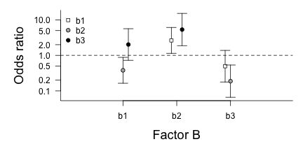
Another useful measure is the odds-ratios. Odds ratios are a measure of the relative odds (probabilities) of events under different scenarios. In this case, we could calculate the odds ratios of a1 vs a2 for each pair of Factor B levels. Odds that deviate substantially from 1 are indicative
> library(biology)
> #We perform pairwise oddsratios on the transposed cross table
> oddsratios(t(dat.xtab))
  Comparison estimate   lower  upper midp.exact fisher.exact chi.square
1   b1 vs b2   2.6374 1.13912 6.1062    0.02466     0.034905   0.021664
2   b1 vs b3   0.4945 0.17734 1.3789    0.18926     0.204734   0.175181
3   b2 vs b3   0.1875 0.06576 0.5346    0.00188     0.002468   0.001056
We could even plot the odds ratios.
> library(biology)
> #Create an empty object in which to store the odds ratios
> or <- NULL
> #Get the colnames from the cross table
> nms <- colnames(dat.xtab)
> #Calculate each pairwise odds ratio
> for (i in 1:ncol(dat.xtab)) {
+     for (j in 1:ncol(dat.xtab)) {
+         if (i == j)
+             next
+         or <- rbind(or, cbind(Comp1 = nms[i], Comp2 = nms[j], oddsratios(dat.xtab[,
+             c(i, j)])))
+     }
+ }
> or$Comp2s <- as.numeric(factor(as.character(or$Comp2)))
> opar <- par(mar = c(5, 6, 1, 1))
> plot(estimate ~ Comp2s, data = or, axes = F, ann = F, type = "n",
+     log = "y", ylim = c(min(or$lower), max(or$upper)), xlim = c(0, 4))
> abline(h = 1, lty = 2)
> with(subset(or, Comp1 == "b1"), arrows(Comp2s - 0.1, lower, Comp2s -
+     0.1, upper, code = 3, length = 0.1, ang = 90))
> points(estimate ~ I(Comp2s - 0.1), data = subset(or, Comp1 == "b1"),
+     type = "p", pch = 22, bg = "white")
> with(subset(or, Comp1 == "b2"), arrows(Comp2s - 0, lower, Comp2s -
+     0, upper, code = 3, length = 0.1, ang = 90))
> points(estimate ~ I(Comp2s - 0), data = subset(or, Comp1 == "b2"),
+     type = "p", pch = 21, bg = "grey70")
> with(subset(or, Comp1 == "b3"), arrows(Comp2s + 0.1, lower, Comp2s +
+     0.1, upper, code = 3, length = 0.1, ang = 90))
> points(estimate ~ I(Comp2s + 0.1), data = subset(or, Comp1 == "b3"),
+     type = "p", pch = 21, bg = "black")
> axis(1, at = 1:3, labels = nms)
> axis(2, las = 1)
> mtext("Factor B", 1, line = 3, cex = 1.5)
> mtext("Odds ratio", 2, line = 3.5, cex = 1.5)
> legend("topleft", legend = nms, pch = c(22, 21, 21), pt.bg = c("white",
+     "grey70", "black"), bty = "n")
> box(bty = "l")