Tutorial 11.4b -Logistic regression
23 April 2011
Binary data
Scenario and Data
Logistic regression is a type of generalized linear model (GLM) that models a binary response against a linear predictor via a specific link function. The linear predictor is the typically a linear combination of effects parameters (e.g. $\beta_0 + \beta_1x_x$). The role of the link function is to transform the expected values of the response y (which is on the scale of (0,1), as is the binomial distribution from which expectations are drawn) into the scale of the linear predictor (which is $-\infty,\infty$). GLM's transform the expected values (via a link) whereas LM's transform the observed data. Thus while GLM's operate on the scale of the original data and yet also on a scale appropriate of the residuals, LM's do neither.
There are many ways (transformations) that can map values on the (0,1) scale into values on the ($-\infty,\infty$) scale, however, the three most common are:
- logit: $log\left(\frac{\pi}{1-\pi}\right)$ - log odds ratio
- probit: $\phi^{-1}(\pi)$ where $\phi^{-1}$ is an inverse normal cumulative density function
- complimentary log-log: $log(-log(1-\pi))$
Lets say we wanted to model the presence/absence of an item ($y$) against a continuous predictor ($x$) As this section is mainly about the generation of artificial data (and not specifically about what to do with the data), understanding the actual details are optional and can be safely skipped. Consequently, I have folded (toggled) this section away.
- the sample size = 20
- the continuous $x$ variable is a random uniform spread of measurements between 1 and 20
- the rate of change in log odds ratio per unit change in x (slope) = 0.5. The magnitude of the slope is an indicator of how abruptly the log odds ratio changes. A very abrupt change would occur if there was very little variability in the trend. That is, a large slope would be indicative of a threshold effect. A lower slope indicates a gradual change in odds ratio and thus a less obvious and precise switch between the likelihood of 1 vs 0.
- the inflection point (point where the slope of the line is greatest) = 10. The inflection point indicates the value of the predictor ($x$) where the log Odds are 50% (switching between 1 being more likely and 0 being more likely). This is also known as the LD50.
- the intercept (which has no real interpretation) is equal to the negative of the slope multiplied by the inflection point
- to generate the values of $y$ expected at each $x$ value, we evaluate the linear predictor. These expected values are then transformed into a scale mapped by (0,1) by using the inverse logit function $\frac{e^{linear~predictor}}{1+e^{linear~predictor}}$
- finally, we generate $y$ values by using the expected $y$ values as probabilities when drawing random numbers from a binomial distribution. This step adds random noise to the expected $y$ values and returns only 1's and 0's.
> set.seed(8)
> # The number of samples
> n.x <- 20
> # Create x values that at uniformly distributed
> # throughout the rate of 1 to 20
> x <- sort(runif(n = n.x, min = 1, max = 20))
> # The slope is the rate of change in log odds ratio
> # for each unit change in x the smaller the slope,
> # the slower the change (more variability in data
> # too)
> slope = 0.5
> # Inflection point is where the slope of the line
> # is greatest this is also the LD50 point
> inflect <- 10
> # Intercept (no interpretation)
> intercept <- -1 * (slope * inflect)
> # The linear predictor
> linpred <- intercept + slope * x
> # Predicted y values
> y.pred <- exp(linpred)/(1 + exp(linpred))
> # Add some noise and make binomial
> n.y <- rbinom(n = n.x, 20, p = 0.9)
> y <- rbinom(n = n.x, size = 1, prob = y.pred)
> dat <- data.frame(y, x)
With these sort of data, we are primarily interested in investigating whether there is a relationship between the binary response variable and the linear predictor (linear combination of one or more continuous or categorical predictors).
Exploratory data analysis and initial assumption checking
- All of the observations are independent - this must be addressed at the design and collection stages
- The response variable (and thus the residuals) should be matched by an appropriate distribution (in the case of a binary response - a binomial is appropriate).
- All observations are equally influential in determining the trends - or at least no observations are overly influential. This is most effectively diagnosed via residuals and other influence indices and is very difficult to diagnose prior to analysis
- the relationship between the linear predictor (right hand side of the regression formula) and the link function should be linear. A scatterplot with smoother can be useful for identifying possible non-linearity.
So lets explore linearity by creating a histogram of the predictor variable ($x$) and a scatterplot of the relationship between the response ($y$) and the predictor ($x$)
> hist(dat$x)

> # now for the scatterplot
> plot(y ~ x, dat)
> with(dat, lines(lowess(y ~ x)))

Conclusions: the predictor ($x$) does not display any skewness or other issues that might lead to non-linearity. The lowess smoother on the scatterplot does not display major deviations from a standard sigmoidal curve and thus linearity is satisfied. Violations of linearity could be addressed by either:
- define a non-linear linear predictor (such as a polynomial, spline or other non-linear function)
- transform the scale of the predictor variables
JAGS
Effects model
Note that in order to prevent arithmetic overflows (particularly with the clog-log model, I am going to constrain the estimated linear predictor to between -20 and 20. Values outside of this on a inverse-log scale are extremely small and huge respectively.I will demonstrate logistic regression with a range of possible link functions (each of which yield different parameter interpretations):
- logit
$$
\begin{array}{rcl}
y &\sim& \operatorname{Bern}(\pi)\\
log\left(\frac{\pi}{1-\pi}\right)&=&\beta_0+\beta_1x_1\\
\beta_0, \beta_1&\sim&\mathcal{N}(0, 10000)\\
\end{array}
$$
> dat.list <- with(dat, list(y=y, x=x, N=nrow(dat)))
> modelString="
model{
  for (i in 1:N) {
    y[i] ~ dbern(p[i])
    logit(p[i]) <- max(-20,min(20,beta0+beta1*x[i]))
  }
  beta0 ~ dnorm(0,1.0E-06)
  beta1 ~ dnorm(0,1.0E-06)
}
"
> writeLines(modelString, con='../downloads/BUGSscripts/tut11.4bS1.bug')
> library(R2jags)
> dat.logit.jags <- jags(data=dat.list,model.file='../downloads/BUGSscripts/tut11.4bS1.bug',
+                    param=c('beta0','beta1'),
+                    n.chains=3, n.iter=20000, n.burnin=10000, n.thin=10)
Compiling model graph
   Resolving undeclared variables
   Allocating nodes
   Graph Size: 147

Initializing model
- probit
$$
\begin{array}{rcl}
y &\sim& \operatorname{Bern}(\pi)\\
\phi^{-1}\left(\pi\right)&=&\beta_0+\beta_1x_1\\
\beta_0, \beta_1&\sim&\mathcal{N}(0, 10000)\\
\end{array}
$$
> dat.list <- with(dat, list(y=y, x=x, N=nrow(dat)))
> modelString="
model{
  for (i in 1:N) {
    y[i] ~ dbern(p[i])
    probit(p[i]) <- max(-20,min(20,beta0+beta1*x[i]))
  }
  beta0 ~ dnorm(0,1.0E-06)
  beta1 ~ dnorm(0,1.0E-06)
}
"
> writeLines(modelString, con='../downloads/BUGSscripts/tut11.4bS1.3b.bug')
> library(R2jags)
> dat.probit.jags <- jags(data=dat.list,model.file='../downloads/BUGSscripts/tut11.4bS1.3b.bug',
+                    param=c('beta0','beta1'),
+                    n.chains=3, n.iter=20000, n.burnin=10000, n.thin=10)
Compiling model graph
   Resolving undeclared variables
   Allocating nodes
   Graph Size: 147

Initializing model
- complimentary log-log
$$
\begin{array}{rcl}
y &\sim& \operatorname{Bern}(\pi)\\
log(-log(1-\pi))&=&\beta_0+\beta_1x_1\\
\beta_0, \beta_1&\sim&\mathcal{N}(0, 10000)\\
\end{array}
$$
> dat.list <- with(dat, list(y=y, x=x, N=nrow(dat)))
> modelString="
model{
  for (i in 1:N) {
    y[i] ~ dbern(p[i])
    cloglog(p[i]) <- max(-20,min(20,beta0+beta1*x[i]))
  }
  beta0 ~ dnorm(0,1.0E-06)
  beta1 ~ dnorm(0,1.0E-06)
}
"
> writeLines(modelString, con='../downloads/BUGSscripts/tut11.4bS1.3c.bug')
> library(R2jags)
> dat.cloglog.jags <- jags(data=dat.list,model.file='../downloads/BUGSscripts/tut11.4bS1.3c.bug',
+                    param=c('beta0','beta1'),
+                    n.chains=3, n.iter=20000, n.burnin=10000, n.thin=10)
Compiling model graph
   Resolving undeclared variables
   Allocating nodes
   Graph Size: 147

Initializing model
>
> dat.glmC <- glm(y~x, data=dat, family=binomial(link="cloglog"))
Chain mixing and Model validation
Prior to exploring the model parameters, it is prudent to confirm that the model did indeed fit the assumptions and was an appropriate fit to the data as well as that the MCMC sampling chain was adequately mixed and the retained samples independent.
Whilst I will only demonstrate this for the logit model, the procedure would be identical for exploring the probit and clog-log models.
- We will start by exploring the mixing of the MCMC chains via traceplots.
> plot(as.mcmc(dat.logit.jags))
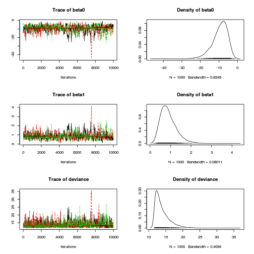
Other than the large spike in one of the chains (not ideal), the chains appear well mixed. Nevertheless, it is clear that the parameters are not symmetrically distributed. Hence, medians might be better descriptors of parameter estimates than means.
- Next we will explore correlation amongst MCMC samples.
> autocorr.diag(as.mcmc(dat.logit.jags))
           beta0    beta1  deviance
Lag 0    1.00000  1.00000  1.000000
Lag 10   0.78467  0.78149  0.468320
Lag 50   0.30114  0.30100  0.187033
Lag 100  0.03986  0.03733  0.067780
Lag 500 -0.04061 -0.03525 -0.009913
It seems that the level of auto-correlation at the nominated lag of 10 is extremely high. Ideally, the level of auto-correlation should be less than 0.1. To achieve this, we need a lag of 1000. Consequently, we will resample at a lag of 1000 and obviously we are going to need more iterations to ensure that we retain a large enough sample from which to derive estimates.
In order to support a thinning rate of 1000, the number of iterations is going to need to be very high. Hence, the following might take considerable time to run.
> library(R2jags)
> dat.logit.jags <- jags(data=dat.list,model.file='../downloads/BUGSscripts/tut11.4bS1.bug',
+                    param=c('beta0','beta1'),
+                    n.chains=3, n.iter=20000, n.burnin=10000, n.thin=100)
Compiling model graph
   Resolving undeclared variables
   Allocating nodes
   Graph Size: 147

Initializing model
> plot(as.mcmc(dat.logit.jags))
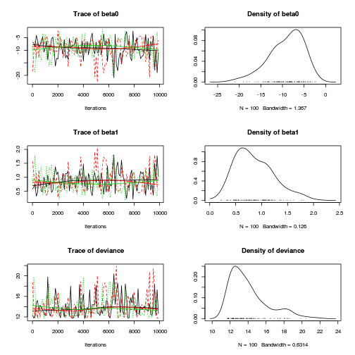
> autocorr.diag(as.mcmc(dat.logit.jags))
             beta0    beta1 deviance
Lag 0     1.000000  1.00000  1.00000
Lag 100   0.078701  0.06203  0.10744
Lag 500   0.005474  0.01466  0.06587
Lag 1000 -0.112558 -0.10794  0.02170
Lag 5000  0.093204  0.07813 -0.01983
Conclusions: the samples are now less auto-correlated and the chains are arguably mixed better.
- We now explore the goodness of fit of the models via the residuals and deviance.
We could calculate the Pearsons's residuals within the JAGS model.
Alternatively, we could use the parameters to generate the residuals outside of JAGS.
> coefs <- dat.logit.jags$BUGSoutput$sims.matrix[,1:2]
> Xmat <- model.matrix(~x, data=dat)
> eta<-coefs %*% t(Xmat)
> pi <- inv.logit(eta)
> #sweep across rows and then divide by pi
> Resid <- -1*sweep(pi,2,dat$y,'-')/sqrt(pi*(1-pi))
> plot(apply(Resid,2,mean)~apply(eta,2,mean))

- Now we will compare the sum of squared residuals to the sum of squares residuals that would be expected from a Bernoulli distribution
matching that estimated by the model. Essentially this is estimating how well the Bernoulli distribution and linear model
approximates the observed data.
Alternatively, we could generate the new samples and calculate the sums squares of residuals etc all within JAGS.
> SSres<-apply(Resid^2,1,sum)
>
> set.seed(2)
> #generate a matrix of draws from a binomial distribution
> # the matrix is the same dimensions as pi and uses the probabilities of pi
> YNew <- matrix(rbinom(length(pi),prob=pi,size=1),nrow=nrow(pi))
>
> Resid1<-(pi - YNew)/sqrt(pi*(1-pi))
> SSres.sim<-apply(Resid1^2,1,sum)
> mean(SSres.sim>SSres)
[1] 0.2497
> dat.list <- with(dat, list(y=y, x=x, N=nrow(dat)))
> modelString="
model{
  for (i in 1:N) {
    y[i] ~ dbern(p[i])
    logit(p[i]) <- max(-20,min(20,eta[i]))
    eta[i] <- beta0+beta1*x[i]
    YNew[i] ~dbern(p[i])
    varY[i] <- p[i]*(1-p[i])
    PRes[i] <- (y[i] - p[i]) / sqrt(varY[i])
    PResNew[i] <- (YNew[i] - p[i]) / sqrt(varY[i])
    D[i] <- pow(PRes[i],2)
    DNew[i] <- pow(PResNew[i],2)
  }
  Fit <- sum(D[1:N])
  FitNew <-sum(DNew[1:N])
  beta0 ~ dnorm(0,1.0E-06)
  beta1 ~ dnorm(0,1.0E-06)
  pvalue <- mean(FitNew>Fit)
}
"
> writeLines(modelString, con='../downloads/BUGSscripts/tut11.4bS5.bug')
> library(R2jags)
> dat.logit.jags1 <- jags(data=dat.list,model.file='../downloads/BUGSscripts/tut11.4bS5.bug',
+                    param=c('beta0','beta1','Fit','FitNew'),
+                    n.chains=3, n.iter=20000, n.burnin=10000, n.thin=10)
Compiling model graph
   Resolving undeclared variables
   Allocating nodes
   Graph Size: 346

Initializing model
> print(dat.logit.jags1)
Inference for Bugs model at "../downloads/BUGSscripts/tut11.4bS5.bug", fit using jags,
 3 chains, each with 20000 iterations (first 10000 discarded), n.thin = 10
 n.sims = 3000 iterations saved
         mu.vect sd.vect    2.5%     25%    50%
Fit       44.036 110.954   9.873  13.003 18.884
FitNew    19.690  88.409   1.924   4.373  7.872
beta0     -9.135   3.661 -17.505 -11.340 -8.622
beta1      0.861   0.343   0.335   0.616  0.810
deviance  13.748   1.984  11.707  12.304 13.150
            75%   97.5%  Rhat n.eff
Fit      35.419 228.548 1.003  1200
FitNew   16.979 103.002 1.001  2700
beta0    -6.496  -3.517 1.003  1100
beta1     1.073   1.635 1.003  1500
deviance 14.552  19.136 1.001  3000

For each parameter, n.eff is a crude measure of effective sample size,
and Rhat is the potential scale reduction factor (at convergence, Rhat=1).

DIC info (using the rule, pD = var(deviance)/2)
pD = 2.0 and DIC = 15.7
DIC is an estimate of expected predictive error (lower deviance is better).
> out <- dat.logit.jags1$BUGSoutput > mean(out$sims.list$FitNew > out$sims.list$Fit)
[1] 0.2663
Conclusions: although the Bayesian p-value is quite a bit lower than 0.5, suggesting that there is more variability in the data than should be expected from this simple logistic regression model, this value is not any closer to 0 (a value that would indicate that the model does not fit the data at all well. Thus we might conclude that whilst not ideal, the model is adequate.
Exploring the model parameters, test hypotheses
If there was any evidence that the assumptions had been violated or the model was not an appropriate fit, then we would need to reconsider the model and start the process again. In this case, there is no evidence that the test will be unreliable so we can proceed to explore the test statistics.
> print(dat.logit.jags)
Inference for Bugs model at "../downloads/BUGSscripts/tut11.4bS1.bug", fit using jags,
 3 chains, each with 2e+05 iterations (first 1e+05 discarded), n.thin = 100
 n.sims = 3000 iterations saved
         mu.vect sd.vect    2.5%     25%    50%
beta0     -9.691   4.246 -19.912 -11.967 -8.960
beta1      0.913   0.396   0.334   0.635  0.846
deviance  13.991   2.276  11.713  12.317 13.288
            75%  97.5%  Rhat n.eff
beta0    -6.695 -3.431 1.001  3000
beta1     1.111  1.863 1.001  3000
deviance 14.932 20.111 1.002  1100

For each parameter, n.eff is a crude measure of effective sample size,
and Rhat is the potential scale reduction factor (at convergence, Rhat=1).

DIC info (using the rule, pD = var(deviance)/2)
pD = 2.6 and DIC = 16.6
DIC is an estimate of expected predictive error (lower deviance is better).
>
> library(plyr)
> adply(dat.logit.jags$BUGSoutput$sims.matrix[,1:2], 2, function(x) {
+   data.frame(Median=median(x), Mean=mean(x), HPDinterval(as.mcmc(x)), HPDinterval(as.mcmc(x),p=0.5))
+ })
     X1  Median    Mean    lower  upper  lower.1
1 beta0 -8.9596 -9.6911 -18.4891 -2.817 -10.8257
2 beta1  0.8461  0.9127   0.2146  1.684   0.5579
  upper.1
1  -5.834
2   1.005
Conclusions:
We would reject the null hypothesis (p<0.05).
An increase in x is associated with a significant linear increase (positive slope) in log odds of $y$ success.
Every 1 unit increase in $x$ results in a 0.7872 unit increase in log odds-ratio.
We usually express this in terms of odds-ratio rather than log odds-ratio, so
every 1 unit increase in $x$ results in a ($e^{0.7872}=2.1972$)
2.1972 unit increase in odds-ratio.
Further explorations of the trends
We might also be interested in the LD50 - the value of $x$ where the probability switches from favoring 1 to favoring 0. LD50 is calculated as: $$LD50 = - \frac{intercept}{slope}$$
> library(coda)
> summary(as.mcmc(-coefs[, 1]/coefs[, 2]))
Iterations = 1:3000
Thinning interval = 1
Number of chains = 1
Sample size per chain = 3000

1. Empirical mean and standard deviation for each variable,
   plus standard error of the mean:

          Mean             SD       Naive SE
       10.6395         1.0888         0.0199
Time-series SE
        0.0199

2. Quantiles for each variable:

 2.5%   25%   50%   75% 97.5%
 8.48  9.97 10.65 11.30 12.86
> # OR
> LD50 <- -coefs[, 1]/coefs[, 2]
> data.frame(Median = median(LD50), Mean = mean(LD50),
+     HPDinterval(as.mcmc(LD50)), HPDinterval(as.mcmc(LD50),
+         p = 0.5))
     Median  Mean lower upper lower.1 upper.1
var1  10.65 10.64 8.568 12.93   10.03   11.34
10.6475.
Finally, we will create a summary plot.
> par(mar = c(4, 5, 0, 0))
> plot(y ~ x, data = dat, type = "n", ann = F, axes = F)
> points(y ~ x, data = dat, pch = 16)
> xs <- seq(0, 20, l = 1000)
>
> Xmat <- model.matrix(~xs)
> eta <- coefs %*% t(Xmat)
> library(boot)
> ys <- inv.logit(eta)
> library(plyr)
> data.tab <- adply(ys, 2, function(x) {
+     data.frame(Median = median(x), HPDinterval(as.mcmc(x)))
+ })
> data.tab <- cbind(x = xs, data.tab)
>
> points(Median ~ x, data = data.tab, col = "black",
+     type = "l")
> lines(lower ~ x, data = data.tab, col = "black", type = "l",
+     lty = 2)
> lines(upper ~ x, data = data.tab, col = "black", type = "l",
+     lty = 2)
> axis(1)
> mtext("X", 1, cex = 1.5, line = 3)
> axis(2, las = 2)
> mtext("Y", 2, cex = 1.5, line = 3)
> box(bty = "l")

Grouped binary data
Scenario and Data
In the previous demonstration, the response variable represented the state of a single item per level of the predictor variable ($x$). That single item could be observed having a value of either 1 or 0. Another common situation is to observe the number of items in one of two states (typically dead or alive) for each level of a treatment. For example, you could tally up the number of germinated and non-germinated seeds out of a bank of 10 seeds at each of 8 temperature or nutrient levels.
Recall that the binomial distribution represents the density (probability) of all possible successes (germinations) out of a total of $N$ items (seeds). Hence the binomial distribution is also a suitable error distribution for such grouped binary data.
For this demonstration, we will model the number of successes against a uniformly distributed predictor ($x$). The number of trials in each group (level of the predictor) will vary slightly (yet randomly) so as to mimick complications that inevadably occur in real experimentws.
- the number of levels of $x$ = 10
- the continuous $x$ variable is a random uniform spread of measurements between 10 and 20
- the rate of change in log odds ratio per unit change in x (slope) = -0.25. The magnitude of the slope is an indicator of how abruptly the log odds ratio changes. A very abrupt change would occur if there was very little variability in the trend. That is, a large slope would be indicative of a threshold effect. A lower slope indicates a gradual change in odds ratio and thus a less obvious and precise switch between the likelihood of 1 vs 0.
- the inflection point (point where the slope of the line is greatest) = 10. The inflection point indicates the value of the predictor ($x$) where the log Odds are 50% (switching between 1 being more likely and 0 being more likely). This is also known as the LD50.
- the intercept (which has no real interpretation) is equal to the negative of the slope multiplied by the inflection point
- generate the values of $y$ expected at each $x$ value, we evaluate the linear predictor.
- generate random numbers of trials per group by drawing integers out of a binomial distribution with a total size of 20 and probability of 0.9. Hence the maximum number of trials per group will be 20, yet some will be less than that.
- the number of success per group are drawn from a binomial distribution with a total size equal to the trial sizes generated in the previous step and probabilities equal to the expected $y$ values
- finally, the number of failures per group are calculated as the difference between the total trial size and number of successes per group.
> set.seed(8)
> # The number of levels of x
> n.x <- 10
> # Create x values that at uniformly distributed
> # throughout the rate of 10 to 20
> x <- sort(runif(n = n.x, min = 10, max = 20))
> # The slope is the rate of change in log odds ratio
> # for each unit change in x the smaller the slope,
> # the slower the change (more variability in data
> # too)
> slope = -0.25
> # Inflection point is where the slope of the line
> # is greatest this is also the LD50 point
> inflect <- 15
> # Intercept (no interpretation)
> intercept <- -1 * (slope * inflect)
> # The linear predictor
> linpred <- intercept + slope * x
> # Predicted y values
> y.pred <- exp(linpred)/(1 + exp(linpred))
> # Add some noise and make binary (0's and 1's)
> n.trial <- rbinom(n = n.x, 20, prob = 0.9)
> success <- rbinom(n = n.x, size = n.trial, prob = y.pred)
> failure <- n.trial - success
> dat <- data.frame(success, failure, x)
Exploratory data analysis and initial assumption checking
- All of the observations are independent - this must be addressed at the design and collection stages
- The response variable (and thus the residuals) should be matched by an appropriate distribution (in the case of a binary response - a binomial is appropriate).
- All observations are equally influential in determining the trends - or at least no observations are overly influential. This is most effectively diagnosed via residuals and other influence indices and is very difficult to diagnose prior to analysis
- the relationship between the linear predictor (right hand side of the regression formula) and the link function should be linear. A scatterplot with smoother can be useful for identifying possible non-linearity.
So lets explore linearity by creating a histogram of the predictor variable ($x$) and a scatterplot of the relationship between the either the number of successes ($success$) or the number of ($failures$) and the predictor ($x$). Note, that this will not account for the differences in trial size per group and so a scatterplot of the relationship between the number of successes ($success$) or the number of ($failures$) divided by the total number of trials against the predictor ($x$) might be more appropriate.
> hist(dat$x)

> # now for the scatterplot
> plot(success ~ x, dat)
> with(dat, lines(lowess(success ~ x)))

> # scatterplot standardized for trial size
> plot(success/(success + failure) ~ x, dat)
> with(dat, lines(lowess(success/(success + failure) ~
+     x)))

Conclusions: the predictor ($x$) does not display any skewness (although it is not all that uniform - random data hey!) or other issues that might lead to non-linearity. The lowess smoother on either scatterplot does not display major deviations from a standard sigmoidal curve and thus linearity is likely to be satisfied. Violations of linearity could be addressed by either:
- define a non-linear linear predictor (such as a polynomial, spline or other non-linear function)
- transform the scale of the predictor variables
Model fitting or statistical analysis - JAGS
Clearly the number of successes is also dependent on the number of trials. Larger numbers of trials might be expected to yeild higher numbers of successes.
> dat.list <- with(dat, list(success=success, total=success+failure, x=x, N=nrow(dat)))
> modelString="
model{
  for (i in 1:N) {
    success[i] ~ dbin(p[i],total[i])
    logit(p[i]) <- max(-20,min(20,beta0+beta1*x[i]))
  }
  beta0 ~ dnorm(0,1.0E-06)
  beta1 ~ dnorm(0,1.0E-06)
}
"
> writeLines(modelString, con='../downloads/BUGSscripts/tut11.4bS2.bug')
> library(R2jags)
> dat.logit.jags <- jags(data=dat.list,model.file='../downloads/BUGSscripts/tut11.4bS2.bug',
+                    param=c('beta0','beta1'),
+                    n.chains=3, n.iter=200000, n.burnin=100000, n.thin=100)
Compiling model graph
   Resolving undeclared variables
   Allocating nodes
   Graph Size: 87

Initializing model
As with the logistic regression presented earlier, we could alternatively use probit or clog-log link functions.
Model evaluation
Prior to exploring the model parameters, it is prudent to confirm that the model did indeed fit the assumptions and was an appropriate fit to the data.
- We will start by exploring the mixing of the MCMC chains via traceplots.
> plot(as.mcmc(dat.logit.jags))
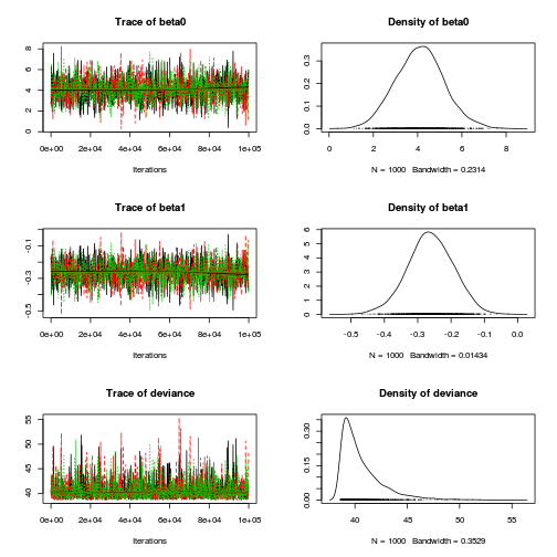
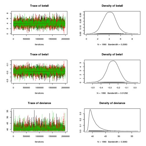
Conclusions: the chains appear well mixed and stable.
- Next we will explore correlation amongst MCMC samples.
> autocorr.diag(as.mcmc(dat.logit.jags))
             beta0     beta1 deviance
Lag 0     1.000000  1.000000 1.000000
Lag 100   0.255541  0.255337 0.042573
Lag 500  -0.006730 -0.013100 0.003285
Lag 1000  0.001617 -0.002010 0.035553
Lag 5000 -0.006401 -0.004475 0.020854
It seems that the level of auto-correlation at the nominated lag of 10 is extremely high. Ideally, the level of auto-correlation should be less than 0.1. To achieve this, we need a lag of 100. Consequently, we will resample at a lag of 100 and obviously we are going to need more iterations to ensure that we retain a large enough sample from which to derive estimates.
> library(R2jags)
> dat.logit.jags <- jags(data=dat.list,model.file='../downloads/BUGSscripts/tut11.4bS2.bug',
+                    param=c('beta0','beta1'),
+                    n.chains=3, n.iter=2000000, n.burnin=10000, n.thin=1000)
Compiling model graph
   Resolving undeclared variables
   Allocating nodes
   Graph Size: 87

Initializing model
> plot(as.mcmc(dat.logit.jags))
> autocorr.diag(as.mcmc(dat.logit.jags))
              beta0     beta1 deviance
Lag 0      1.000000  1.000000  1.00000
Lag 1000   0.013149  0.013054 -0.01071
Lag 5000   0.020145  0.018079  0.01088
Lag 10000 -0.004512 -0.002863 -0.00351
Lag 50000  0.007128  0.008616 -0.01168
-
Lets explore the diagnostics - particularly the residuals
Conclusions: there is no obvious patterns in the residuals, or at least there are no obvious trends remaining that would be indicative of non-linearity.> # Calculate residuals > coefs <- dat.logit.jags$BUGSoutput$sims.matrix[, 1:2] > Xmat <- model.matrix(~x, data = dat) > eta <- coefs %*% t(Xmat) > pi <- inv.logit(eta) > # sweep across rows and then divide by pi > Resid <- -1 * sweep(pi, 2, dat$success/(dat$success + + dat$failure), "-")/sqrt(pi * (1 - pi)) > plot(apply(Resid, 2, mean) ~ apply(eta, 2, mean)) > lines(lowess(apply(Resid, 2, mean) ~ apply(eta, 2, + mean)))

- Now we will compare the sum of squared residuals to the sum of squares residuals that would be expected from a Bernoulli distribution
matching that estimated by the model. Essentially this is estimating how well the Bernoulli distribution and linear model
approximates the observed data.
> SSres<-apply(Resid^2,1,sum)
>
> set.seed(2)
> #generate a matrix of draws from a binomial distribution
> # the matrix is the same dimensions as pi and uses the probabilities of pi
> YNew <- matrix(rbinom(length(pi),prob=pi,size=(dat$success+dat$failure)),nrow=nrow(pi))
> Resid1 <- 1*(pi-YNew/(dat$success+dat$failure))/sqrt(pi*(1-pi))
> SSres.sim<-apply(Resid1^2,1,sum)
> mean(SSres.sim>SSres)
[1] 0.6419
Conclusions: this Bayesian p-value is reasonably close to 0.5. Therefore we would conclude that there was no strong evidence for a lack of fit of the model.
Further explorations of the trends
We might also be interested in the LD50 - the value of $x$ where the probability switches from favoring 1 to favoring 0. LD50 is calculated as: $$LD50 = - \frac{intercept}{slope}$$
> library(coda)
> summary(as.mcmc(-coefs[, 1]/coefs[, 2]))
Iterations = 1:5970
Thinning interval = 1
Number of chains = 1
Sample size per chain = 5970

1. Empirical mean and standard deviation for each variable,
   plus standard error of the mean:

          Mean             SD       Naive SE
      15.66993        0.69043        0.00894
Time-series SE
       0.00894

2. Quantiles for each variable:

 2.5%   25%   50%   75% 97.5%
 14.3  15.3  15.7  16.1  17.0
> # OR
> LD50 <- -coefs[, 1]/coefs[, 2]
> data.frame(Median = median(LD50), Mean = mean(LD50),
+     HPDinterval(as.mcmc(LD50)), HPDinterval(as.mcmc(LD50),
+         p = 0.5))
     Median  Mean lower upper lower.1 upper.1
var1  15.69 15.67 14.36 17.05   15.29    16.1
15.6932.
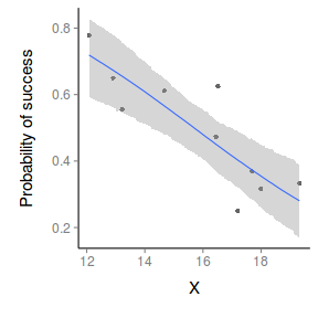
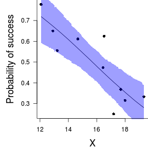
Finally, we will create a summary plot.
> par(mar = c(4, 5, 0, 0))
> plot(success/(success + failure) ~ x, data = dat, type = "n",
+     ann = F, axes = F)
> points(success/(success + failure) ~ x, data = dat,
+     pch = 16)
> xs <- seq(min(dat$x, na.rm = TRUE), max(dat$x, na.rm = TRUE),
+     l = 1000)
>
> Xmat <- model.matrix(~xs)
> eta <- coefs %*% t(Xmat)
> library(boot)
> ys <- inv.logit(eta)
> library(plyr)
> data.tab <- adply(ys, 2, function(x) {
+     data.frame(Median = median(x), HPDinterval(as.mcmc(x)))
+ })
> data.tab <- cbind(x = xs, data.tab)
>
> points(Median ~ x, data = data.tab, col = "black",
+     type = "l")
> with(data.tab, polygon(c(x, rev(x)), c(lower, rev(upper)),
+     col = "#0000ff60", border = NA))
> # lines(lower ~ x, data=data.tab,col = 'black',
> # type = 'l', lty = 2) lines(upper ~ x,
> # data=data.tab,col = 'black', type = 'l', lty = 2)
> axis(1)
> mtext("X", 1, cex = 1.5, line = 3)
> axis(2, las = 2)
> mtext("Probability of success", 2, cex = 1.5, line = 3)
> box(bty = "l")
> xs <- seq(min(dat$x, na.rm = TRUE), max(dat$x, na.rm = TRUE),
+     l = 1000)
> Xmat <- model.matrix(~xs)
> eta <- coefs %*% t(Xmat)
> library(boot)
> ys <- inv.logit(eta)
> library(plyr)
> data.tab <- adply(ys, 2, function(x) {
+     data.frame(Median = median(x), HPDinterval(as.mcmc(x)))
+ })
> data.tab <- cbind(x = xs, data.tab)
>
> library(ggplot2)
> library(grid)
> dat$p <- with(dat, success/(success + failure))
> p1 <- ggplot(data.tab, aes(y = Median, x = x)) + geom_point(data = dat,
+     aes(y = p, x = x), color = "gray40") + geom_smooth(aes(ymin = lower,
+     ymax = upper), stat = "identity") + scale_x_continuous("X") +
+     scale_y_continuous("Probability of success")
> p1 + theme(panel.grid.major = element_blank(), panel.grid.minor = element_blank(),
+     panel.border = element_blank(), panel.background = element_blank(),
+     axis.title.y = element_text(size = 15, vjust = 0,
+         angle = 90), axis.title.x = element_text(size = 15,
+         vjust = -1), axis.text.y = element_text(size = 12),
+     axis.text.x = element_text(size = 12), axis.line = theme_segment(),
+     plot.margin = unit(c(0.5, 0.5, 2, 2), "lines"))
