Tutorial 11.5a - Poisson regression and log-linear models
23 April 2011
Poisson regression
Poisson regression is a type of generalized linear model (GLM) that models a positive integer (natural number) response against a linear predictor via a specific link function. The linear predictor is typically a linear combination of effects parameters (e.g. $\beta_0 + \beta_1x_x$). The role of the link function is to transform the expected values of the response y (which is on the scale of (0,$\infty$), as is the Poisson distribution from which expectations are drawn) into the scale of the linear predictor (which is $-\infty,\infty$).
As implied in the name of this group of analyses, a Poisson rather than Gaussian (normal) distribution is used to represent the errors (residuals). Like count data (number of individuals, species etc), the Poisson distribution encapsulates positive integers and is bound by zero at one end. Consequently, the degree of variability is directly related the expected value (equivalent to the mean of a Gaussian distribution). Put differently, the variance is a function of the mean. Repeated observations from a Poisson distribution located close to zero will yield a much smaller spread of observations than will samples drawn from a Poisson distribution located a greater distance from zero. In the Poisson distribution, the variance has a 1:1 relationship with the mean.
The canonical link function for the Poisson distribution is a log-link function.
Whilst the expectation that the mean=variance ($\mu=\sigma$) is broadly compatible with actual count data (that variance increases at the same rate as the mean), under certain circumstances, this might not be the case. For example, when there are other unmeasured influences on the response variable, the distribution of counts might be somewhat clumped which can result in higher than expected variability (that is $\sigma\gt\mu$). The variance increases more rapidly than does the mean. This is referred to as overdispersion. The degree to which the variability is greater than the mean (and thus the expected degree of variability) is called dispersion. Effectively, the Poisson distribution has a dispersion parameter (or scaling factor) of 1.
It turns out that overdispersion is very common for count data and it typically underestimates variability, standard errors and thus deflated p-values. There are a number of ways of overcoming this limitation, the effectiveness of which depend on the causes of overdispersion.
- Quasi-Poisson models - these introduce the dispersion parameter ($\phi$) into the model.
This approach does not utilize an underlying error distribution to calculate the maximum likelihood (there is no quasi-Poisson distribution).
Instead, if the Newton-Ralphson iterative reweighting least squares algorithm is applied using a direct specification of the relationship between
mean and variance ($var(y)=\phi\mu$), the estimates of the regression coefficients are identical to those of the maximum
likelihood estimates from the Poisson model. This is analogous to fitting ordinary least squares on symmetrical, yet not normally distributed data -
the parameter estimates are the same, however they won't necessarily be as efficient.
The standard errors of the coefficients are then calculated by multiplying the Poisson model coefficient
standard errors by $\sqrt{\phi}$.
Unfortunately, because the quasi-poisson model is not estimated via maximum likelihood, properties such as AIC and log-likelihood cannot be derived. Consequently, quasi-poisson and Poisson model fits cannot be compared via either AIC or likelihood ratio tests (nor can they be compared via deviance as uasi-poisson and Poisson models have the same residual deviance). That said, quasi-likelihood can be obtained by dividing the likelihood from the Poisson model by the dispersion (scale) factor.
- Negative binomial model - technically, the negative binomial distribution is a probability distribution for the number of successes before a specified number of failures.
However, the negative binomial can also be defined (parameterized) in terms of a mean ($\mu$) and scale factor ($\omega$),
$$p(y_i)=\frac{\Gamma(y_i+\omega)}{\Gamma(\omega)y!}\times\frac{\mu_i^{y_i}\omega^\omega}{(\mu_i+\omega)^{\mu_i+\omega}}$$
where the expectected value of the values $y_i$ (the means) are ($mu_i$) and the variance is $y_i=\frac{\mu_i+\mu_i^2}{\omega}$.
In this way, the negative binomial is a two-stage hierarchical process in which the response is modeled against a Poisson distribution whose expected count is in turn
modeled by a Gamma distribution with a mean of $\mu$ and constant scale parameter ($\omega$).
Strictly, the negative binomial is not an exponential family distribution (unless $\omega$ is fixed as a constant), and thus negative binomial models cannot be fit via the usual GLM iterative reweighting algorithm. Instead estimates of the regression parameters along with the scale factor ($\omega$) are obtained via maximum likelihood.
The negative binomial model is useful for accommodating overdispersal when it is likely caused by clumping (due to the influence of other unmeasured factors) within the response.
- Zero-inflated Poisson model - overdispersion can also be caused by the presence of a greater number of zero's than would otherwise be expected for a Poisson distribution.
There are potentially two sources of zero counts - genuine zeros and false zeros.
Firstly, there may genuinely be no individuals present. This would be the number expected by a Poisson distribution.
Secondly, individuals may have been present yet not detected or may not even been possible.
These are false zero's and lead to zero inflated data (data with more zeros than expected).
For example, the number of joeys accompanying an adult koala could be zero because the koala has no offspring (true zero) or because the koala is male or infertile (both of which would be examples of false zeros). Similarly, zero counts of the number of individual in a transect are due either to the absence of individuals or the inability of the observer to detect them. Whilst in the former example, the latent variable representing false zeros (sex or infertility) can be identified and those individuals removed prior to analysis, this is not the case for the latter example. That is, we cannot easily partition which counts of zero are due to detection issues and which are a true indication of the natural state.
Consistent with these two sources of zeros, zero-inflated models combine a binary logistic regression model (that models count membership according to a latent variable representing observations that can only be zeros - not detectable or male koalas) with a Poisson regression (that models count membership according to a latent variable representing observations whose values could be 0 or any positive integer - fertile female koalas).
Poisson regression
Scenario and Data
Lets say we wanted to model the abundance of an item ($y$) against a continuous predictor ($x$). As this section is mainly about the generation of artificial data (and not specifically about what to do with the data), understanding the actual details are optional and can be safely skipped. Consequently, I have folded (toggled) this section away.
- the sample size = 20
- the continuous $x$ variable is a random uniform spread of measurements between 1 and 20
- the rate of change in log $y$ per unit of $x$ (slope) = 0.1.
- the value of $x$ when log$y$ equals 0 (when $y$=1)
- to generate the values of $y$ expected at each $x$ value, we evaluate the linear predictor (created by calculating the outer product of the model matrix and the regression parameters). These expected values are then transformed into a scale mapped by (0,$\infty$) by using the log function $e^{linear~predictor}$
- finally, we generate $y$ values by using the expected $y$ values ($\lambda$) as probabilities when drawing random numbers from a Poisson distribution. This step adds random noise to the expected $y$ values and returns only 0's and positive integers.
> set.seed(8)
> # The number of samples
> n.x <- 20
> # Create x values that at uniformly distributed throughout the rate of 1 to 20
> x <- sort(runif(n = n.x, min = 1, max = 20))
> mm <- model.matrix(~x)
> intercept <- 0.6
> slope = 0.1
> # The linear predictor
> linpred <- mm %*% c(intercept, slope)
> # Predicted y values
> lambda <- exp(linpred)
> # Add some noise and make binomial
> y <- rpois(n = n.x, lambda = lambda)
> dat <- data.frame(y, x)
> data.pois <- dat
> write.table(data.pois, file = "../downloads/data/data.pois.csv", quote = F, row.names = F, sep = ",")
With these sort of data, we are primarily interested in investigating whether there is a relationship between the positive integer response variable and the linear predictor (linear combination of one or more continuous or categorical predictors).
Exploratory data analysis and initial assumption checking
- All of the observations are independent - this must be addressed at the design and collection stages
- The response variable (and thus the residuals) should be matched by an appropriate distribution (in the case of positive integers response - a Poisson is appropriate).
- All observations are equally influential in determining the trends - or at least no observations are overly influential. This is most effectively diagnosed via residuals and other influence indices and is very difficult to diagnose prior to analysis
- the relationship between the linear predictor (right hand side of the regression formula) and the link function should be linear. A scatterplot with smoother can be useful for identifying possible non-linearity.
- The dispersion factor is close to 1
There are five main potential models we could consider fitting to these data:
- Ordinary least squares regression (general linear model) - assumes normality of residuals
- Poisson regression - assumes mean=variance (dispersion=1)
- Quasi-poisson regression - a general solution to overdispersion. Assumes variance is a function of mean, dispersion estimated, however likelihood based statistics unavailable
- Negative binomial regression - a specific solution to overdispersion caused by clumping (due to an unmeasured latent variable). Scaling factor ($\omega$) is estimated along with the regression parameters.
- Zero-inflation model - a specific solution to overdispersion caused by excessive zeros (due to an unmeasured latent variable). Mixture of binomial and Poisson models.
Confirm non-normality and explore clumping
When counts are all very large (not close to 0) and their ranges do not span orders of magnitude, they take on very Gaussian properties (symmetrical distribution and variance independent of the mean). Given that models based on the Gaussian distribution are more optimized and recognized than Generalized Linear Models, it can be prudent to adopt Gaussian models for such data. Hence it is a good idea to first explore whether a Poisson model is likely to be more appropriate than a standard Gaussian model.
The potential for overdispersion can be explored by adding a rug to boxplot. The rug is simply tick marks on the inside of an axis at the position corresponding to an observation. As multiple identical values result in tick marks drawn over one another, it is typically a good idea to apply a slight amount of jitter (random displacement) to the values used by the rug.
> hist(dat$y)

> boxplot(dat$y, horizontal = TRUE)
> rug(jitter(dat$y), side = 1)

Confirm linearity
Lets now explore linearity by creating a histogram of the predictor variable ($x$) and a scatterplot of the relationship between the response ($y$) and the predictor ($x$)
> hist(dat$x)

> # now for the scatterplot
> plot(y ~ x, dat, log = "y")
> with(dat, lines(lowess(y ~ x)))

Conclusions: the predictor ($x$) does not display any skewness or other issues that might lead to non-linearity. The lowess smoother on the scatterplot does not display major deviations from a straight line and thus linearity is satisfied. Violations of linearity could be addressed by either:
- define a non-linear linear predictor (such as a polynomial, spline or other non-linear function)
- transform the scale of the predictor variables
Explore zero inflation
Although we have already established that there are few zeros in the data (and thus overdispersion is unlikely to be an issue), we can also explore this by comparing the number of zeros in the data to the number of zeros that would be expected from a Poisson distribution with a mean equal to the mean count of the data.
> # proportion of 0's in the data
> dat.tab <- table(dat$y == 0)
> dat.tab/sum(dat.tab)
FALSE
    1
> # proportion of 0's expected from a Poisson distribution
> mu <- mean(dat$y)
> cnts <- rpois(1000, mu)
> dat.tab <- table(cnts == 0)
> dat.tab/sum(dat.tab)
FALSE  TRUE
0.997 0.003
Model fitting or statistical analysis
We perform the Poisson regression using the glm() function. The most important (=commonly used) parameters/arguments for logistic regression are:
- formula: the linear model relating the response variable to the linear predictor
- family: specification of the error distribution (and link function).
Can be specified as either a string or as one of the family functions (which allows for the explicit declaration of the link function).
For examples:
- family="poisson" or equivalently family=poisson(link="log")
- data: the data frame containing the data
I will now fit the Poisson regression: $$log(\mu)=\beta_0+\beta_1x_1+\epsilon_i, \hspace{1cm}\epsilon\sim Poisson(\lambda)$$
> dat.glm <- glm(y ~ x, data = dat, family = "poisson")
Model evaluation
Prior to exploring the model parameters, it is prudent to confirm that the model did indeed fit the assumptions and was an appropriate fit to the data. There are a number of extractor functions (functions that extract or derive specific information from a model) available including:
| Extractor | Description |
|---|---|
| residuals() | Extracts the residuals from the model |
| fitted() | Extracts the predicted (expected) response values (on the link scale) at the observed levels of the linear predictor |
| predict() | Extracts the predicted (expected) response values (on either the link, response or terms (linear predictor) scale) |
| coef() | Extracts the model coefficients |
| deviance() | Extracts the deviance from the model |
| AIC() | Extracts the Akaike's Information Criterion from the model |
| extractAIC() | Extracts the generalized Akaike's Information Criterion from the model |
| summary() | Summarizes the important output and characteristics of the model |
| anova() | Computes an analysis of deviance or log-likelihood ratio test (LRT) from the model |
| plot() | Generates a series of diagnostic plots from the model |
Lets explore the diagnostics - particularly the residuals
> plot(dat.glm)
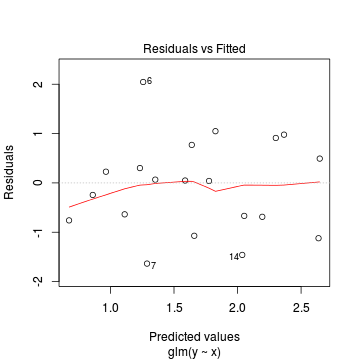

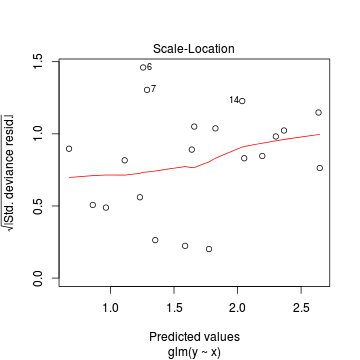
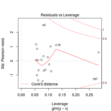
Goodness of fit of the model
We can also explore the goodness of the fit of the model via:
- Pearson's $\chi^2$ residuals
- explores whether there are any significant patterns remaining in the residuals
> dat.resid <- sum(resid(dat.glm, type = "pearson")^2)
> 1 - pchisq(dat.resid, dat.glm$df.resid)
[1] 0.4897
- Deviance ($G^2$) - similar to the $\chi^2$ test above, yet uses deviance
Conclusions: neither Pearson residuals or Deviance indicate a lack of fit (p values greater than 0.05)> 1 - pchisq(dat.glm$deviance, dat.glm$df.resid)
[1] 0.5076
In this demonstration we fitted the Poisson model. We could also compare (using AIC or deviance) its fit to that of a Gaussian model.
Conclusions: from the perspective of both AIC and deviance, the Poisson model would be considered a better fit to the data.> dat.glmG <- glm(y ~ x, data = dat, family = "gaussian") > AIC(dat.glm, dat.glmG)
         df   AIC
dat.glm   2 90.32
dat.glmG  3 98.28
> # Poisson deviance
> dat.glm$deviance
[1] 17.23
> # Gaussian deviance
> dat.glmG$deviance
[1] 118.1
Dispersion
Recall that the Poisson regression model assumes that variance=mean ($var=\mu\phi$ where $\phi=1$) and thus dispersion ($\phi=\frac{var}{\mu}=1$). However, we can also calculate approximately what the dispersion factor would be by using the model deviance as a measure of variance and the model residual degrees of freedom as a measure of the mean (since the expected value of a Poisson distribution is the same as its degrees of freedom). $$\phi=\frac{Deviance}{df}$$
Conclusion: the estimated dispersion parameter is very close to 1 thereby confirming that overdispersion is unlikely to be an issue.> dat.glm$deviance/dat.glm$df.resid
[1] 0.957
> # Or alternatively, via Pearson's residuals
> Resid <- resid(dat.glm, type = "pearson")
> sum(Resid^2)/(nrow(dat) - length(coef(dat.glm)))
[1] 0.9717
Exploring the model parameters, test hypotheses
If there was any evidence that the assumptions had been violated or the model was not an appropriate fit, then we would need to reconsider the model and start the process again. In this case, there is no evidence that the test will be unreliable so we can proceed to explore the test statistics. The main statistic of interest is the Wald statistic ($z$) for the slope parameter.
> summary(dat.glm)
Call:
glm(formula = y ~ x, family = "poisson", data = dat)

Deviance Residuals:
   Min      1Q  Median      3Q     Max
-1.635  -0.705   0.044   0.562   2.046

Coefficients:
            Estimate Std. Error z value Pr(>|z|)
(Intercept)   0.5600     0.2539    2.21    0.027 *
x             0.1115     0.0186    6.00    2e-09 ***
---
Signif. codes:  0 '***' 0.001 '**' 0.01 '*' 0.05 '.' 0.1 ' ' 1

(Dispersion parameter for poisson family taken to be 1)

    Null deviance: 55.614  on 19  degrees of freedom
Residual deviance: 17.226  on 18  degrees of freedom
AIC: 90.32

Number of Fisher Scoring iterations: 4
Conclusions: We would reject the null hypothesis (p<0.05). An increase in x is associated with a significant linear increase (positive slope) in log $y$ abundance. Every 1 unit increase in $x$ is associated with a 0.1115 unit increase in $\log y$ abundance We usually express this in terms of $y$ than $\log y$, so every 1 unit increase in $x$ is associated with a ($e^{0.1115}=1.12$) 1.12 unit increase in $y$ abundance.
P-values are widely acknowledged as a rather flawed means of inference testing (as in hypothesis testing in general). An alternate way of exploring the characteristics of parameter estimates is to calculate their confidence intervals. Confidence intervals that do not overlap with the null hypothesis parameter value (e.g. effect of 0), are an indication of a significant effect. Recall however, that in frequentist statistics the confidence intervals are interpreted as the range of values that are likely to contain the true mean on 95 out of 100 (95%) repeated samples.
Conclusions: A 1 unit increase in $x$ is associated with a ($e^{0.1115}=1.12$) 1.12 (1.08,1.16) unit increase in $y$ abundance.> library(gmodels) > ci(dat.glm)
            Estimate CI lower CI upper Std. Error   p-value
(Intercept)   0.5600  0.02649   1.0935    0.25395 2.744e-02
x             0.1115  0.07247   0.1506    0.01858 1.971e-09
Further explorations of the trends
A measure of the strength of the relationship can be obtained according to: $$quasi R^2 = 1-\left(\frac{deviance}{null~deviance}\right)$$
Conclusions: approximately> 1 - (dat.glm$deviance/dat.glm$null)
[1] 0.6903
69% of the variability in abundance can be explained by its relationship to $x$. Technically, it is69% of the variability in $\log y$ (the link function) is explained by its relationship to $x$.Finally, we will create a summary plot.
> par(mar = c(4, 5, 0, 0))
> plot(y ~ x, data = dat, type = "n", ann = F, axes = F)
> points(y ~ x, data = dat, pch = 16)
> xs <- seq(0, 20, l = 1000)
> ys <- predict(dat.glm, newdata = data.frame(x = xs), type = "response", se = T)
> points(ys$fit ~ xs, col = "black", type = "l")
> lines(ys$fit - 1 * ys$se.fit ~ xs, col = "black", type = "l", lty = 2)
> lines(ys$fit + 1 * ys$se.fit ~ xs, col = "black", type = "l", lty = 2)
> axis(1)
> mtext("X", 1, cex = 1.5, line = 3)
> axis(2, las = 2)
> mtext("Abundance of Y", 2, cex = 1.5, line = 3)
> box(bty = "l")

Quasi-Poisson regression
Lets say we wanted to model the abundance of an item ($y$) against a continuous predictor ($x$). As this section is mainly about the generation of artificial data (and not specifically about what to do with the data), understanding the actual details are optional and can be safely skipped. Consequently, I have folded (toggled) this section away.
Random data incorporating the following trends (effect parameters)- define a function that will generate random samples from a quasi-poisson distribution $$QuasiPoisson\left(\frac{\mu}{\phi-1}, \frac{1}{\phi}\right)$$ where $\mu$ is the expected value (mean) and $\phi$ is the dispersion factor such that $var(y)=\phi\mu$.
- the sample size = 20
- the continuous $x$ variable is a random uniform spread of measurements between 1 and 20
- the rate of change in log $y$ per unit of $x$ (slope) = 0.1.
- the value of $x$ when log$y$ equals 0 (when $y$=1)
- to generate the values of $y$ expected at each $x$ value, we evaluate the linear predictor (created by calculating the outer product of the model matrix and the regression parameters). These expected values are then transformed into a scale mapped by (0,$\infty$) by using the log function $e^{linear~predictor}$
- finally, we generate $y$ values by using the expected $y$ values ($\lambda$) as probabilities when drawing random numbers from a quasi-poisson distribution. This step adds random noise to the expected $y$ values and returns only 0's and positive integers.
> # Quasi-poisson distrition
> rqpois <- function(n, lambda, phi) {
+     mu = lambda
+     r = rnbinom(n, size = mu/phi/(1 - 1/phi), prob = 1/phi)
+     return(r)
+ }
>
> set.seed(8)
> # The number of samples
> n.x <- 20
> # Create x values that at uniformly distributed throughout the rate of 1 to 20
> x <- sort(runif(n = n.x, min = 1, max = 20))
> mm <- model.matrix(~x)
> intercept <- 0.6
> slope = 0.1
> # The linear predictor
> linpred <- mm %*% c(intercept, slope)
> # Predicted y values
> lambda <- exp(linpred)
> # Add some noise and make binomial
> y <- rqpois(n = n.x, lambda = lambda, phi = 4)
> dat.qp <- data.frame(y, x)
> data.qp <- dat.qp
> write.table(data.qp, file = "../downloads/data/data.qp.csv", quote = F, row.names = F, sep = ",")
Exploratory data analysis and initial assumption checking
The assumptions are:- All of the observations are independent - this must be addressed at the design and collection stages
- The response variable (and thus the residuals) should be matched by an appropriate distribution (in the case of positive integers response - a Poisson is appropriate).
- All observations are equally influential in determining the trends - or at least no observations are overly influential. This is most effectively diagnosed via residuals and other influence indices and is very difficult to diagnose prior to analysis
- the relationship between the linear predictor (right hand side of the regression formula) and the link function should be linear. A scatterplot with smoother can be useful for identifying possible non-linearity.
- Dispersion is either 1 or overdispersion is accounted for in the model and is not due to excessive clumping or zero-inflation
Recall from Poisson regression, there are five main potential models that we could consider fitting to these data.
There are five main potential models we could consider fitting to these data:
- Ordinary least squares regression (general linear model) - assumes normality of residuals
- Poisson regression - assumes mean=variance (dispersion=1)
- Quasi-poisson regression - a general solution to overdispersion. Assumes variance is a function of mean, dispersion estimated, however likelihood based statistics unavailable
- Negative binomial regression - a specific solution to overdispersion caused by clumping (due to an unmeasured latent variable). Scaling factor ($\omega$) is estimated along with the regression parameters.
- Zero-inflation model - a specific solution to overdispersion caused by excessive zeros (due to an unmeasured latent variable). Mixture of binomial and Poisson models.
Confirm non-normality and explore clumping
Check the distribution of the $y$ abundances
There is definitely signs of non-normality that would warrant some form of Poisson model. There is also some evidence of clumping that might result in overdispersion. Some zero values are present, yet there are not so many that we would be concerned about zero-inflation.> hist(dat.qp$y)

> boxplot(dat.qp$y, horizontal = TRUE)
> rug(jitter(dat.qp$y), side = 1)

Confirm linearity
Lets now explore linearity by creating a histogram of the predictor variable ($x$) and a scatterplot of the relationship between the response ($y$) and the predictor ($x$)
> hist(dat.qp$x)

> # now for the scatterplot
> plot(y ~ x, dat.qp, log = "y")
> with(dat.qp, lines(lowess(y ~ x)))

Conclusions: the predictor ($x$) does not display any skewness or other issues that might lead to non-linearity. The lowess smoother on the scatterplot does not display major deviations from a straight line and thus linearity is satisfied. Violations of linearity could be addressed by either:
- define a non-linear linear predictor (such as a polynomial, spline or other non-linear function)
- transform the scale of the predictor variables
Explore zero inflation
Although we have already established that there are few zeros in the data (and thus overdispersion is unlikely to be an issue), we can also explore this by comparing the number of zeros in the data to the number of zeros that would be expected from a Poisson distribution with a mean equal to the mean count of the data.
In the above, the value under FALSE is the proportion of non-zero values in the data and the value under TRUE is the proportion of zeros in the data. In this example, there appears to be a higher proportion of zeros than would be expected. However, if we consider the small sample size of the observed data ($n=20$), there are still only a small number of zeros (> # proportion of 0's in the data > dat.qp.tab <- table(dat.qp$y == 0) > dat.qp.tab/sum(dat.qp.tab)
FALSE  TRUE
 0.85  0.15
> # proportion of 0's expected from a Poisson distribution
> mu <- mean(dat.qp$y)
> cnts <- rpois(1000, mu)
> dat.qp.tabE <- table(cnts == 0)
> dat.qp.tabE/sum(dat.qp.tabE)
FALSE  TRUE
0.997 0.003
3). Nevertheless, a slight excess of zeros might also contribute to overdispersion.Model fitting or statistical analysis
A number of properties of the data during exploratory data analysis have suggested that overdispersion could be an issue. There is a hint of clumping of the response variable and there are also more zeros than we might have expected. At this point, we could consider which of these issues were likely to most severely impact on the fit of the models (clumping or excessive zeros) and fit a model that specifically addresses the issue (negative binomial, zero-inflated Poisson or even zero-inflated binomial). Alternatively, we could perform the Quasi-Poisson regression (which is a more general approach) using the glm() function. The most important (=commonly used) parameters/arguments for logistic regression are:
- formula: the linear model relating the response variable to the linear predictor
- family: specification of the error distribution (and link function).
Can be specified as either a string or as one of the family functions (which allows for the explicit declaration of the link function).
For examples:
- family="quasipoisson" or equivalently family=quasipoisson(link="log")
- data: the data frame containing the data
I will now fit the Quasi-Poisson regression: $$log(\mu)=\beta_0+\beta_1x_1+\epsilon_i, \hspace{1cm}var(y)=\omega\mu$$
> dat.qp.glm <- glm(y ~ x, data = dat.qp, family = "quasipoisson")
Model evaluation
Prior to exploring the model parameters, it is prudent to confirm that the model did indeed fit the assumptions and was an appropriate fit to the data. There are a number of extractor functions (functions that extract or derive specific information from a model) available including:
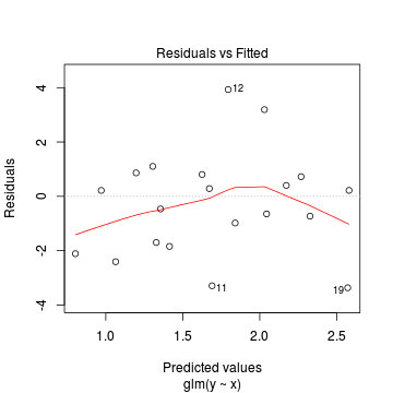
Extractor Description residuals() Extracts the residuals from the model fitted() Extracts the predicted (expected) response values (on the link scale) at the observed levels of the linear predictor predict() Extracts the predicted (expected) response values (on either the link, response or terms (linear predictor) scale) coef() Extracts the model coefficients deviance() Extracts the deviance from the model summary() Summarizes the important output and characteristics of the model anova() Computes an analysis of deviance or log-likelihood ratio test (LRT) from the model plot() Generates a series of diagnostic plots from the model Lets explore the diagnostics - particularly the residuals
Conclusions: there is no obvious patterns in the residuals, or at least there are no obvious trends remaining that would be indicative of non-linearity. None of the observations are considered overly influential (Cooks' D values not approaching 1).> plot(dat.qp.glm)

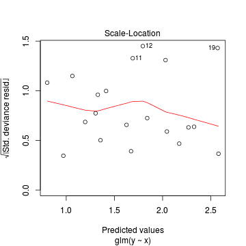
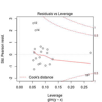
Since the regression coefficients are estimated directly from maximum likelihood without taking into account an error distribution, genuine log-likelihoods are not calculated. Consequently, derived model comparison metrics such as AIC are not formally available. Furthermore, as both Poisson and Quasi-Poisson models yield identical deviance, we cannot compare the fit of the quasi-poisson to a Poisson model via deviance either
> dat.p.glm <- glm(y ~ x, data = dat.qp, family = "poisson")
> # Poisson deviance
> dat.p.glm$deviance
[1] 69.99
> # Quasi-poisson deviance
> dat.qp.glm$deviance
[1] 69.99
Exploring the model parameters, test hypotheses
If there was any evidence that the assumptions had been violated or the model was not an appropriate fit, then we would need to reconsider the model and start the process again. In this case, there is no evidence that the test will be unreliable so we can proceed to explore the test statistics. The main statistic of interest is the t-statistic ($t$) for the slope parameter.
> summary(dat.qp.glm)
Call:
glm(formula = y ~ x, family = "quasipoisson", data = dat.qp)

Deviance Residuals:
   Min      1Q  Median      3Q     Max
-3.366  -1.736  -0.124   0.744   3.933

Coefficients:
            Estimate Std. Error t value Pr(>|t|)
(Intercept)   0.6997     0.4746    1.47    0.158
x             0.1005     0.0353    2.85    0.011 *
---
Signif. codes:  0 '***' 0.001 '**' 0.01 '*' 0.05 '.' 0.1 ' ' 1

(Dispersion parameter for quasipoisson family taken to be 3.699)

    Null deviance: 101.521  on 19  degrees of freedom
Residual deviance:  69.987  on 18  degrees of freedom
AIC: NA

Number of Fisher Scoring iterations: 5
Conclusions: Note the dispersion (scale) factor is estimated as 3.699. Whilst this is greater than zero (thus confirming overdispersion), it would not be considered a large degree of overdispersion. So although negative binomial and zero-inflation models are typically preferred over Quasi-Poisson models (as they address the causes of overdispersion more directly), in this case, it is unlikely to make much difference.
We would reject the null hypothesis (p<0.05). An increase in x is associated with a significant linear increase (positive slope) in log $y$ abundance. Every 1 unit increase in $x$ is associated with a 0.1005 unit increase in $\log y$ abundance We usually express this in terms of $y$ than $\log y$, so every 1 unit increase in $x$ is associated with a ($e^{0.1}=1.11$) 1.11 unit increase in $y$ abundance.
P-values are widely acknowledged as a rather flawed means of inference testing (as in hypothesis testing in general). An alternate way of exploring the characteristics of parameter estimates is to calculate their confidence intervals. Confidence intervals that do not overlap with the null hypothesis parameter value (e.g. effect of 0), are an indication of a significant effect. Recall however, that in frequentist statistics the confidence intervals are interpreted as the range of values that are likely to contain the true mean on 95 out of 100 (95%) repeated samples.
Conclusions: A 1 unit increase in $x$ is associated with a ($e^{0.1005}=1.11$) 1.11 (1.03,1.19) unit increase in $y$ abundance.> library(gmodels) > ci(dat.qp.glm)
            Estimate CI lower CI upper Std. Error p-value
(Intercept)   0.6997 -0.29744   1.6967     0.4746 0.15770
x             0.1005  0.02632   0.1746     0.0353 0.01071
Note that if we compare the Quasi-poisson parameter estimates to those of a Poisson, they have identical point estimates yet the Quasi-poisson model yields wider standard errors and confident intervals reflecting the greater variability modeled. In fact, the standard error of the Quasi-poisson model regression coefficients will be $\sqrt{\phi}$ times greater than those of the Poisson model. ($0.035 = \sqrt{3.699}\times 0.0184$).
> summary(dat.p.glm <- glm(y ~ x, data = dat.qp, family = "poisson"))
Call:
glm(formula = y ~ x, family = "poisson", data = dat.qp)

Deviance Residuals:
   Min      1Q  Median      3Q     Max
-3.366  -1.736  -0.124   0.744   3.933

Coefficients:
            Estimate Std. Error z value Pr(>|z|)
(Intercept)   0.6997     0.2468    2.84   0.0046 **
x             0.1005     0.0184    5.47  4.4e-08 ***
---
Signif. codes:  0 '***' 0.001 '**' 0.01 '*' 0.05 '.' 0.1 ' ' 1

(Dispersion parameter for poisson family taken to be 1)

    Null deviance: 101.521  on 19  degrees of freedom
Residual deviance:  69.987  on 18  degrees of freedom
AIC: 134.9

Number of Fisher Scoring iterations: 5
> ci(dat.p.glm)
            Estimate CI lower CI upper Std. Error   p-value
(Intercept)   0.6997  0.18121    1.218    0.24677 4.579e-03
x             0.1005  0.06192    0.139    0.01835 4.389e-08
Further explorations of the trends
A measure of the strength of the relationship can be obtained according to: $$quasi R^2 = 1-\left(\frac{deviance}{null~deviance}\right)$$
Conclusions: approximately> 1 - (dat.qp.glm$deviance/dat.qp.glm$null)
[1] 0.3106
31.1% of the variability in abundance can be explained by its relationship to $x$. Technically, it is31.1% of the variability in $\log y$ (the link function) is explained by its relationship to $x$.Finally, we will create a summary plot.
> par(mar = c(4, 5, 0, 0))
> plot(y ~ x, data = dat.qp, type = "n", ann = F, axes = F)
> points(y ~ x, data = dat.qp, pch = 16)
> xs <- seq(0, 20, l = 1000)
> ys <- predict(dat.qp.glm, newdata = data.frame(x = xs), type = "response", se = T)
> points(ys$fit ~ xs, col = "black", type = "l")
> lines(ys$fit - 1 * ys$se.fit ~ xs, col = "black", type = "l", lty = 2)
> lines(ys$fit + 1 * ys$se.fit ~ xs, col = "black", type = "l", lty = 2)
> axis(1)
> mtext("X", 1, cex = 1.5, line = 3)
> axis(2, las = 2)
> mtext("Abundance of Y", 2, cex = 1.5, line = 3)
> box(bty = "l")

Observation-level random effect
One of the 'causes' of an overdispersed model is that important unmeasured (latent) effect(s) have not been incorporated. That is, there are one or more unobserved influences that result in a greater amount of variability in the response than would be expected from the Poisson distribution. We could attempt to 'mop up' this addition variation by adding a latent effect as a observation-level random effect in the model.
This random effect is just a numeric vector containing a sequence of integers from 1 to the number of observations. It acts as a proxy for the latent effects.
We will use the same data as the previous section on Quasipoisson to demonstrate observation-level random effects. Consequently, the exploratory data analysis section is the same as above (and therefore not repeated here).
Model fitting or statistical analysis
In order to incorporate observation-level random effects, we must use generalized linear mixed effects modelling. For this example, we will use the lme() function of the nlme package. The most important (=commonly used) parameters/arguments for logistic regression are:
- fixed: the linear model relating the response variable to the fixed component of the linear predictor
- random: the linear model relating the response variable to the random component of the linear predictor
- family: specification of the error distribution (and link function).
Can be specified as either a string or as one of the family functions (which allows for the explicit declaration of the link function).
For examples:
- family="poisson" or equivalently family=poisson(link="log")
- data: the data frame containing the data
I will now fit the observation-level random effects Poisson regression: $$log(\mu)=\beta_0+\beta_1x_1+Z\beta_2+\epsilon_i, \hspace{1cm}var(y)=\omega\mu$$
> dat.qp$units <- 1:nrow(dat.qp)
> library(MASS)
> dat.qp.glmm <- glmmPQL(y ~ x, random = ~1 | units, data = dat.qp, family = "poisson")
Model evaluation
Prior to exploring the model parameters, it is prudent to confirm that the model did indeed fit the assumptions and was an appropriate fit to the data. There are a number of extractor functions (functions that extract or derive specific information from a model) available including:
Extractor Description residuals() Extracts the residuals from the model fitted() Extracts the predicted (expected) response values (on the link scale) at the observed levels of the linear predictor predict() Extracts the predicted (expected) response values (on either the link, response or terms (linear predictor) scale) coef() Extracts the model coefficients fixef() Extracts the model coefficients of the fixed components ranef() Extracts the model coefficients of the fixed components deviance() Extracts the deviance from the model summary() Summarizes the important output and characteristics of the model anova() Computes an analysis of deviance or log-likelihood ratio test (LRT) from the model plot() Generates a series of diagnostic plots from the model Lets explore the diagnostics - particularly the residuals
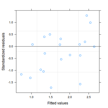
Conclusions: there is no obvious patterns in the residuals.> plot(dat.qp.glmm)
> dat.qp.resid <- sum(resid(dat.qp.glmm, type = "pearson")^2)
> 1 - pchisq(dat.qp.resid, dat.qp.glmm$fixDF$X[2])
[1] 0.7033
Exploring the model parameters, test hypotheses
If there was any evidence that the assumptions had been violated or the model was not an appropriate fit, then we would need to reconsider the model and start the process again. In this case, there is no evidence that the test will be unreliable so we can proceed to explore the test statistics. The main statistic of interest is the t-statistic ($t$) for the slope parameter.
> summary(dat.qp.glmm)
Linear mixed-effects model fit by maximum likelihood
 Data: dat.qp
  AIC BIC logLik
   NA  NA     NA

Random effects:
 Formula: ~1 | units
        (Intercept) Residual
StdDev:      0.3998    1.503

Variance function:
 Structure: fixed weights
 Formula: ~invwt
Fixed effects: y ~ x
             Value Std.Error DF t-value p-value
(Intercept) 0.7367    0.5000 18   1.473  0.1579
x           0.1021    0.0392 18   2.601  0.0181
 Correlation:
  (Intr)
x -0.935

Standardized Within-Group Residuals:
    Min      Q1     Med      Q3     Max
-1.7187 -0.9891 -0.1497  0.2235  1.2896

Number of Observations: 20
Number of Groups: 20
Conclusions: We would reject the null hypothesis (p<0.05). An increase in x is associated with a significant linear increase (positive slope) in log $y$ abundance. Every 1 unit increase in $x$ is associated with a 0.1021 unit increase in $\log y$ abundance We usually express this in terms of $y$ than $\log y$, so every 1 unit increase in $x$ is associated with a ($e^{0.1}=1.11$) 1.11 unit increase in $y$ abundance.
As indicated, P-values are widely acknowledged as a rather flawed means of inference testing (as in hypothesis testing in general). This is further exacerbated with mixed effects models. An alternate way of exploring the characteristics of parameter estimates is to calculate their confidence intervals. Confidence intervals that do not overlap with the null hypothesis parameter value (e.g. effect of 0), are an indication of a significant effect. Recall however, that in frequentist statistics the confidence intervals are interpreted as the range of values that are likely to contain the true mean on 95 out of 100 (95%) repeated samples.
Conclusions: A 1 unit increase in $x$ is associated with a ($e^{0.1021}=1.107$) 1.11 (1.02,1.20) unit increase in $y$ abundance.> library(gmodels) > ci(dat.qp.glmm)
            Estimate CI lower CI upper Std. Error DF p-value
(Intercept)   0.7367 -0.31372   1.7870    0.49996 18 0.15791
x             0.1021  0.01962   0.1845    0.03924 18 0.01806
Compared to either the Quasi-Poisson or the simple Poisson models fitted above, the observation-level random effects model, has substantially larger standard errors and confidence intervals (in this case) reflecting the greater variability built in to the model.
> summary(dat.p.glm <- glm(y ~ x, data = dat.qp, family = "poisson"))
Call:
glm(formula = y ~ x, family = "poisson", data = dat.qp)

Deviance Residuals:
   Min      1Q  Median      3Q     Max
-3.366  -1.736  -0.124   0.744   3.933

Coefficients:
            Estimate Std. Error z value Pr(>|z|)
(Intercept)   0.6997     0.2468    2.84   0.0046 **
x             0.1005     0.0184    5.47  4.4e-08 ***
---
Signif. codes:  0 '***' 0.001 '**' 0.01 '*' 0.05 '.' 0.1 ' ' 1

(Dispersion parameter for poisson family taken to be 1)

    Null deviance: 101.521  on 19  degrees of freedom
Residual deviance:  69.987  on 18  degrees of freedom
AIC: 134.9

Number of Fisher Scoring iterations: 5
> ci(dat.p.glm)
            Estimate CI lower CI upper Std. Error   p-value
(Intercept)   0.6997  0.18121    1.218    0.24677 4.579e-03
x             0.1005  0.06192    0.139    0.01835 4.389e-08
Finally, we will create a summary plot.
> par(mar = c(4, 5, 0, 0))
> plot(y ~ x, data = dat.qp, type = "n", ann = F, axes = F)
> points(y ~ x, data = dat.qp, pch = 16)
> xs <- seq(0, 20, l = 1000)
> coefs <- fixef(dat.qp.glmm)
> mm <- model.matrix(~x, data = data.frame(x = xs))
> ys <- as.vector(coefs %*% t(mm))
> se <- sqrt(diag(mm %*% vcov(dat.qp.glmm) %*% t(mm)))
> lwr <- exp(ys - qt(0.975, dat.qp.glmm$fixDF$X[2]) * se)
> upr <- exp(ys + qt(0.975, dat.qp.glmm$fixDF$X[2]) * se)
> lwr50 <- exp(ys - se)
> upr50 <- exp(ys + se)
>
> points(exp(ys) ~ xs, col = "black", type = "l")
> # lines(lwr ~ xs, col = 'black', type = 'l', lty = 2) lines(upr ~ xs, col = 'black', type = 'l', lty
> # = 2)
> lines(lwr50 ~ xs, col = "black", type = "l", lty = 2)
> lines(upr50 ~ xs, col = "black", type = "l", lty = 2)
> axis(1)
> mtext("X", 1, cex = 1.5, line = 3)
> axis(2, las = 2)
> mtext("Abundance of Y", 2, cex = 1.5, line = 3)
> box(bty = "l")

Negative binomial regression
Scenario and Data
Lets say we wanted to model the abundance of an item ($y$) against a continuous predictor ($x$). As this section is mainly about the generation of artificial data (and not specifically about what to do with the data), understanding the actual details are optional and can be safely skipped. Consequently, I have folded (toggled) this section away.
Random data incorporating the following trends (effect parameters)- the sample size = 20
- the continuous $x$ variable is a random uniform spread of measurements between 1 and 20
- the rate of change in log $y$ per unit of $x$ (slope) = 0.1.
- the value of $x$ when log$y$ equals 0 (when $y$=1)
- to generate the values of $y$ expected at each $x$ value, we evaluate the linear predictor (created by calculating the outer product of the model matrix and the regression parameters). These expected values are then transformed into a scale mapped by (0,$\infty$) by using the log function $e^{linear~predictor}$
- finally, we generate $y$ values by using the expected $y$ values ($\lambda$) as probabilities when drawing random numbers from a Poisson distribution. This step adds random noise to the expected $y$ values and returns only 0's and positive integers.
> set.seed(37)  #16 #35
> # The number of samples
> n.x <- 20
> # Create x values that at uniformly distributed throughout the rate of 1 to 20
> x <- sort(runif(n = n.x, min = 1, max = 20))
> mm <- model.matrix(~x)
> intercept <- 0.6
> slope = 0.1
> # The linear predictor
> linpred <- mm %*% c(intercept, slope)
> # Predicted y values
> lambda <- exp(linpred)
> # Add some noise and make binomial
> y <- rnbinom(n = n.x, mu = lambda, size = 1)
> dat.nb <- data.frame(y, x)
> data.nb <- dat.nb
> write.table(data.nb, file = "../downloads/data/data.nb.csv", quote = F, row.names = F, sep = ",")
Exploratory data analysis and initial assumption checking
The assumptions are:- All of the observations are independent - this must be addressed at the design and collection stages
- The response variable (and thus the residuals) should be matched by an appropriate distribution (in the case of positive integers response - a Poisson is appropriate).
- All observations are equally influential in determining the trends - or at least no observations are overly influential. This is most effectively diagnosed via residuals and other influence indices and is very difficult to diagnose prior to analysis
- the relationship between the linear predictor (right hand side of the regression formula) and the link function should be linear. A scatterplot with smoother can be useful for identifying possible non-linearity.
- Dispersion is either 1 or overdispersion is otherwise accounted for in the model
- The number of zeros is either not excessive or else they are specifically addressed by the model
When counts are all very large (not close to 0) and their ranges do not span orders of magnitude, they take on very Gaussian properties (symmetrical distribution and variance independent of the mean). Given that models based on the Gaussian distribution are more optimized and recognized than Generalized Linear Models, it can be prudent to adopt Gaussian models for such data. Hence it is a good idea to first explore whether a Poisson model is likely to be more appropriate than a standard Gaussian model.
Recall from Poisson regression, there are five main potential models that we could consider fitting to these data.
There are five main potential models we could consider fitting to these data:
- Ordinary least squares regression (general linear model) - assumes normality of residuals
- Poisson regression - assumes mean=variance (dispersion=1)
- Quasi-poisson regression - a general solution to overdispersion. Assumes variance is a function of mean, dispersion estimated, however likelihood based statistics unavailable
- Negative binomial regression - a specific solution to overdispersion caused by clumping (due to an unmeasured latent variable). Scaling factor ($\omega$) is estimated along with the regression parameters.
- Zero-inflation model - a specific solution to overdispersion caused by excessive zeros (due to an unmeasured latent variable). Mixture of binomial and Poisson models.
Confirm non-normality and explore clumping
Check the distribution of the $y$ abundances
There is definitely signs of non-normality that would warrant Poisson models. Further to that, the rug on the boxplot is suggestive of clumping (observations are not evenly distributed and well spaced out). Together the, skewness and clumping could point to an overdispersed Poisson. Negative binomial models are the most effective at modeling such data.> hist(dat.nb$y)

> boxplot(dat.nb$y, horizontal = TRUE)
> rug(jitter(dat.nb$y))

Confirm linearity
Lets now explore linearity by creating a histogram of the predictor variable ($x$) and a scatterplot of the relationship between the response ($y$) and the predictor ($x$)
> hist(dat.nb$x)

> # now for the scatterplot
> plot(y ~ x, dat.nb, log = "y")
> with(dat.nb, lines(lowess(y ~ x)))

Conclusions: the predictor ($x$) does not display any skewness or other issues that might lead to non-linearity. The lowess smoother on the scatterplot does not display major deviations from a straight line and thus linearity is satisfied. Violations of linearity could be addressed by either:
- define a non-linear linear predictor (such as a polynomial, spline or other non-linear function)
- transform the scale of the predictor variables
Explore zero inflation
Although we have already established that there are few zeros in the data (and thus overdispersion is unlikely to be an issue), we can also explore this by comparing the number of zeros in the data to the number of zeros that would be expected from a Poisson distribution with a mean equal to the mean count of the data.
In the above, the value under FALSE is the proportion of non-zero values in the data and the value under TRUE is the proportion of zeros in the data. In this example, the proportion of zeros observed is similar to the proportion expected. Indeed, there was only a single zero observed. Hence it is likely that if there is overdispersion it is unlikely to be due to excessive zeros.> # proportion of 0's in the data > dat.nb.tab <- table(dat.nb$y == 0) > dat.nb.tab/sum(dat.nb.tab)
FALSE  TRUE
 0.95  0.05
> # proportion of 0's expected from a Poisson distribution
> mu <- mean(dat.nb$y)
> cnts <- rpois(1000, mu)
> dat.nb.tabE <- table(cnts == 0)
> dat.nb.tabE/sum(dat.nb.tabE)
FALSE 1Model fitting or statistical analysis
The boxplot of $y$ with the axis rug suggested that there might be some clumping (possibly due to some other unmeasured influence). We will therefore perform negative binomial regression using the glm.nb() function. The most important (=commonly used) parameters/arguments for negative binomial regression are:
- formula: the linear model relating the response variable to the linear predictor
- data: the data frame containing the data
I will now fit the negative binomial regression: $$log(\mu)=\beta_0+\beta_1x_1+\epsilon_i, \hspace{1cm}\epsilon\sim NB(\lambda, \phi)$$
> library(MASS)
> dat.nb.glm <- glm.nb(y ~ x, data = dat.nb)
Model evaluation
Prior to exploring the model parameters, it is prudent to confirm that the model did indeed fit the assumptions and was an appropriate fit to the data. There are a number of extractor functions (functions that extract or derive specific information from a model) available including:
Extractor Description residuals() Extracts the residuals from the model fitted() Extracts the predicted (expected) response values (on the link scale) at the observed levels of the linear predictor predict() Extracts the predicted (expected) response values (on either the link, response or terms (linear predictor) scale) coef() Extracts the model coefficients deviance() Extracts the deviance from the model AIC() Extracts the Akaike's Information Criterion from the model extractAIC() Extracts the generalized Akaike's Information Criterion from the model summary() Summarizes the important output and characteristics of the model anova() Computes an analysis of deviance or log-likelihood ratio test (LRT) from the model plot() Generates a series of diagnostic plots from the model Lets explore the diagnostics - particularly the residuals
Conclusions: there is no obvious patterns in the residuals, or at least there are no obvious trends remaining that would be indicative of non-linearity. None of the observations are considered overly influential (Cooks' D values not approaching 1).> plot(dat.nb.glm)
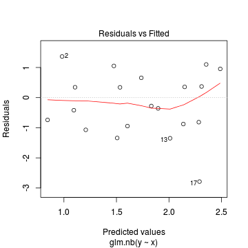
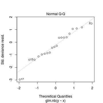
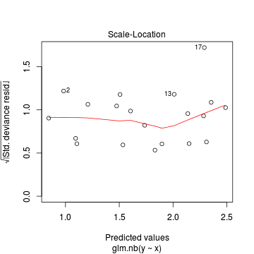
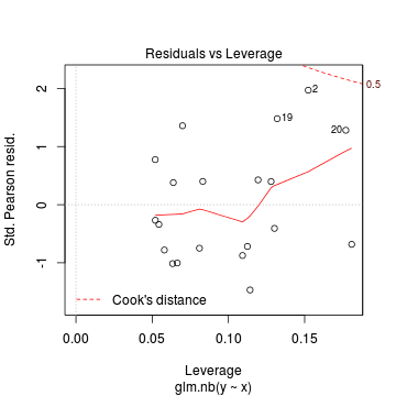
In this demonstration we fitted the Negative binomial model. As well as estimating the regression coefficients, the negative binomial also estimates the dispersion parameter ($\phi$), thus requiring an additional degree of freedom. We could compare the fit of the negative binomial to that of a regular Poisson model (that assumes a dispersion of 1), using AIC.
Conclusions: The AIC is smaller for the Negative binomial model, suggesting that it is a better fit than the Poisson model.> dat.glm <- glm(y ~ x, data = dat.nb, family = "poisson") > AIC(dat.nb.glm, dat.glm)
           df   AIC
dat.nb.glm  3 115.8
dat.glm     2 137.2
Exploring the model parameters, test hypotheses
If there was any evidence that the assumptions had been violated or the model was not an appropriate fit, then we would need to reconsider the model and start the process again. In this case, there is no evidence that the test will be unreliable so we can proceed to explore the test statistics. The main statistic of interest is the Wald statistic ($z$) for the slope parameter.
> summary(dat.nb.glm)
Call:
glm.nb(formula = y ~ x, data = dat.nb, init.theta = 2.359878187,
    link = log)

Deviance Residuals:
   Min      1Q  Median      3Q     Max
-2.787  -0.894  -0.317   0.442   1.366

Coefficients:
            Estimate Std. Error z value Pr(>|z|)
(Intercept)   0.7454     0.4253    1.75   0.0797 .
x             0.0949     0.0344    2.76   0.0058 **
---
Signif. codes:  0 '***' 0.001 '**' 0.01 '*' 0.05 '.' 0.1 ' ' 1

(Dispersion parameter for Negative Binomial(2.36) family taken to be 1)

    Null deviance: 30.443  on 19  degrees of freedom
Residual deviance: 21.806  on 18  degrees of freedom
AIC: 115.8

Number of Fisher Scoring iterations: 1


              Theta:  2.36
          Std. Err.:  1.10

 2 x log-likelihood:  -109.85
Conclusions: We would reject the null hypothesis (p<0.05). An increase in x is associated with a significant linear increase (positive slope) in log $y$ abundance. Every 1 unit increase in $x$ is associated with a 0.1115 unit increase in $\log y$ abundance We usually express this in terms of $y$ than $\log y$, so every 1 unit increase in $x$ is associated with a ($e^{0.1115}=1.12$) 1.12 unit increase in $y$ abundance.
P-values are widely acknowledged as a rather flawed means of inference testing (as in hypothesis testing in general). An alternate way of exploring the characteristics of parameter estimates is to calculate their confidence intervals. Confidence intervals that do not overlap with the null hypothesis parameter value (e.g. effect of 0), are an indication of a significant effect. Recall however, that in frequentist statistics the confidence intervals are interpreted as the range of values that are likely to contain the true mean on 95 out of 100 (95%) repeated samples.
Conclusions: A 1 unit increase in $x$ is associated with a ($e^{0.62}=1.89$) 1.89 (1.14,3.02) unit increase in $y$ abundance.> library(gmodels) > ci(dat.nb.glm)
            Estimate CI lower CI upper Std. Error  p-value
(Intercept)  0.74543 -0.14818   1.6390    0.42534 0.079682
x            0.09494  0.02265   0.1672    0.03441 0.005792
Further explorations of the trends
A measure of the strength of the relationship can be obtained according to: $$quasi R^2 = 1-\left(\frac{deviance}{null~deviance}\right)$$
Conclusions: approximately> 1 - (dat.nb.glm$deviance/dat.nb.glm$null)
[1] 0.2837
28.4% of the variability in abundance can be explained by its relationship to $x$. Technically, it is28.4% of the variability in $\log y$ (the link function) is explained by its relationship to $x$.Finally, we will create a summary plot.
> par(mar = c(4, 5, 0, 0))
> plot(y ~ x, data = dat.nb, type = "n", ann = F, axes = F)
> points(y ~ x, data = dat.nb, pch = 16)
> xs <- seq(0, 20, l = 1000)
> ys <- predict(dat.nb.glm, newdata = data.frame(x = xs), type = "response", se = T)
> points(ys$fit ~ xs, col = "black", type = "l")
> lines(ys$fit - 1 * ys$se.fit ~ xs, col = "black", type = "l", lty = 2)
> lines(ys$fit + 1 * ys$se.fit ~ xs, col = "black", type = "l", lty = 2)
> axis(1)
> mtext("X", 1, cex = 1.5, line = 3)
> axis(2, las = 2)
> mtext("Abundance of Y", 2, cex = 1.5, line = 3)
> box(bty = "l")

Zero-inflation Poisson (ZIP) regression
Scenario and Data
Lets say we wanted to model the abundance of an item ($y$) against a continuous predictor ($x$). As this section is mainly about the generation of artificial data (and not specifically about what to do with the data), understanding the actual details are optional and can be safely skipped. Consequently, I have folded (toggled) this section away.
Random data incorporating the following trends (effect parameters)- the sample size = 20
- the continuous $x$ variable is a random uniform spread of measurements between 1 and 20
- the rate of change in log $y$ per unit of $x$ (slope) = 0.1.
- the value of $x$ when log$y$ equals 0 (when $y$=1)
- to generate the values of $y$ expected at each $x$ value, we evaluate the linear predictor (created by calculating the outer product of the model matrix and the regression parameters). These expected values are then transformed into a scale mapped by (0,$\infty$) by using the log function $e^{linear~predictor}$
- finally, we generate $y$ values by using the expected $y$ values ($\lambda$) as probabilities when drawing random numbers from a Poisson distribution. This step adds random noise to the expected $y$ values and returns only 0's and positive integers.
> set.seed(37)  #34.5  #4 #10 #16 #17 #26
> # The number of samples
> n.x <- 20
> # Create x values that at uniformly distributed throughout the rate of 1 to 20
> x <- sort(runif(n = n.x, min = 1, max = 20))
> mm <- model.matrix(~x)
> intercept <- 0.6
> slope = 0.1
> # The linear predictor
> linpred <- mm %*% c(intercept, slope)
> # Predicted y values
> lambda <- exp(linpred)
> # Add some noise and make binomial
> library(gamlss.dist)
> # fixed latent binomial
> y <- rZIP(n.x, lambda, 0.4)
> # latent binomial influenced by the linear predictor y<- rZIP(n.x,lambda,
> # 1-exp(linpred)/(1+exp(linpred)))
> dat.zip <- data.frame(y, x)
>
> data.zip <- dat.zip
> write.table(data.zip, file = "../downloads/data/data.zip.csv", quote = F, row.names = F, sep = ",")
>
> summary(glm(y ~ x, dat.zip, family = "poisson"))
Call:
glm(formula = y ~ x, family = "poisson", data = dat.zip)

Deviance Residuals:
   Min      1Q  Median      3Q     Max
-2.541  -2.377  -0.975   1.174   3.638

Coefficients:
            Estimate Std. Error z value Pr(>|z|)
(Intercept)   0.6705     0.3302    2.03    0.042 *
x             0.0296     0.0266    1.11    0.266
---
Signif. codes:  0 '***' 0.001 '**' 0.01 '*' 0.05 '.' 0.1 ' ' 1

(Dispersion parameter for poisson family taken to be 1)

    Null deviance: 85.469  on 19  degrees of freedom
Residual deviance: 84.209  on 18  degrees of freedom
AIC: 124

Number of Fisher Scoring iterations: 6
> plot(glm(y ~ x, dat.zip, family = "poisson"))
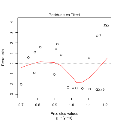

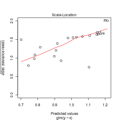
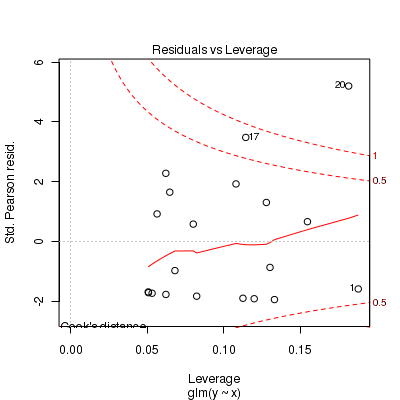
>
> library(pscl)
> summary(zeroinfl(y ~ x | 1, dist = "poisson", data = dat.zip))
Call:
zeroinfl(formula = y ~ x | 1, data = dat.zip, dist = "poisson")

Pearson residuals:
   Min     1Q Median     3Q    Max
-1.001 -0.956 -0.393  0.966  1.619

Count model coefficients (poisson with log link):
            Estimate Std. Error z value Pr(>|z|)
(Intercept)   0.7047     0.3196    2.21  0.02745 *
x             0.0873     0.0253    3.45  0.00056 ***

Zero-inflation model coefficients (binomial with logit link):
            Estimate Std. Error z value Pr(>|z|)
(Intercept)   -0.229      0.456    -0.5     0.62
---
Signif. codes:  0 '***' 0.001 '**' 0.01 '*' 0.05 '.' 0.1 ' ' 1

Number of iterations in BFGS optimization: 13
Log-likelihood: -36.2 on 3 Df
> plot(resid(zeroinfl(y ~ x | 1, dist = "poisson", data = dat.zip)) ~ fitted(zeroinfl(y ~ x | 1, dist = "poisson", + data = dat.zip)))

>
> library(gamlss)
> summary(gamlss(y ~ x, data = dat.zip, family = ZIP))
GAMLSS-RS iteration 1: Global Deviance = 72.44
GAMLSS-RS iteration 2: Global Deviance = 72.34
GAMLSS-RS iteration 3: Global Deviance = 72.34
*******************************************************************
Family:  c("ZIP", "Poisson Zero Inflated")

Call:  gamlss(formula = y ~ x, family = ZIP, data = dat.zip)

Fitting method: RS()

-------------------------------------------------------------------
Mu link function:  log
Mu Coefficients:
             Estimate  Std. Error  t value  Pr(>|t|)
(Intercept)    0.7058      0.3196     2.21   0.04123
x              0.0872      0.0253     3.44   0.00311

-------------------------------------------------------------------
Sigma link function:  logit
Sigma Coefficients:
  Estimate  Std. Error     t value    Pr(>|t|)
    -0.229       0.456      -0.502       0.622

-------------------------------------------------------------------
No. of observations in the fit:  20
Degrees of Freedom for the fit:  3
      Residual Deg. of Freedom:  17
                      at cycle:  3

Global Deviance:     72.34
            AIC:     78.34
            SBC:     81.33
*******************************************************************
> > predict(gamlss(y ~ x, data = dat.zip, family = ZIP), se.fit = TRUE, what = "mu")
GAMLSS-RS iteration 1: Global Deviance = 72.44
GAMLSS-RS iteration 2: Global Deviance = 72.34
GAMLSS-RS iteration 3: Global Deviance = 72.34
$fit
     1      2      3      4      5      6      7      8      9     10     11     12     13     14
0.7967 0.9236 1.0264 1.0370 1.1305 1.3763 1.4054 1.4300 1.4951 1.6161 1.7036 1.7630 1.8679 1.9838
    15     16     17     18     19     20
1.9952 2.1187 2.1250 2.1432 2.1837 2.3065

$se.fit
     1      2      3      4      5      6      7      8      9     10     11     12     13     14
0.3518 0.3089 0.2759 0.2726 0.2446 0.1856 0.1807 0.1771 0.1697 0.1656 0.1710 0.1783 0.1973 0.2252
    15     16     17     18     19     20
0.2282 0.2638 0.2657 0.2713 0.2840 0.3242
Exploratory data analysis and initial assumption checking
The assumptions are:- All of the observations are independent - this must be addressed at the design and collection stages
- The response variable (and thus the residuals) should be matched by an appropriate distribution (in the case of positive integers response - a Poisson is appropriate).
- All observations are equally influential in determining the trends - or at least no observations are overly influential. This is most effectively diagnosed via residuals and other influence indices and is very difficult to diagnose prior to analysis
- the relationship between the linear predictor (right hand side of the regression formula) and the link function should be linear. A scatterplot with smoother can be useful for identifying possible non-linearity.
- Dispersion is either 1 or overdispersion is otherwise accounted for in the model
- The number of zeros is either not excessive or else they are specifically addressed by the model
Confirm non-normality and explore clumping
Check the distribution of the $y$ abundances
There is definitely signs of non-normality that would warrant Poisson models. Further to that, there appears to be a large number of zeros that are likely to be the cause of overdispersion A zero-inflated Poisson model is likely to be one of the most effective for modeling these data.> hist(dat.zip$y)

> boxplot(dat.zip$y, horizontal = TRUE)
> rug(jitter(dat.zip$y))

Confirm linearity
Lets now explore linearity by creating a histogram of the predictor variable ($x$). Note, it is difficult to directly assess issues of linearity. Indeed, a scatterplot with lowess smoother will be largely influenced by the presence of zeros. One possible way of doing so is to explore the trend in the non-zero data.
> hist(dat.zip$x)

> # now for the scatterplot
> plot(y ~ x, dat.zip, log = "y")
> with(subset(dat.zip, y > 0), lines(lowess(y ~ x)))

Conclusions: the predictor ($x$) does not display any skewness or other issues that might lead to non-linearity. The lowess smoother on the non-zero data cloud does not display major deviations from a straight line and thus linearity is likely to be satisfied. Violations of linearity (whilst difficult to be certain about due to the unknown influence of the zeros) could be addressed by either:
- define a non-linear linear predictor (such as a polynomial, spline or other non-linear function)
- transform the scale of the predictor variables
Explore zero inflation
Although we have already established that there are few zeros in the data (and thus overdispersion is unlikely to be an issue), we can also explore this by comparing the number of zeros in the data to the number of zeros that would be expected from a Poisson distribution with a mean equal to the mean count of the data.
In the above, the value under FALSE is the proportion of non-zero values in the data and the value under TRUE is the proportion of zeros in the data. In this example, the proportion of zeros observed (45%) far exceeds that that would have been expected (8%). Hence it is highly likely that any models will be zero-inflated.> # proportion of 0's in the data > dat.zip.tab <- table(dat.zip$y == 0) > dat.zip.tab/sum(dat.zip.tab)
FALSE  TRUE
 0.55  0.45
> # proportion of 0's expected from a Poisson distribution
> mu <- mean(dat.zip$y)
> cnts <- rpois(1000, mu)
> dat.zip.tabE <- table(cnts == 0)
> dat.zip.tabE/sum(dat.zip.tabE)
FALSE  TRUE
0.921 0.079
Model fitting or statistical analysis
The exploratory data analyses have suggested that a zero-inflated Poisson model might be the most appropriate for these data. Zero-inflated models can be fit via functions from one of two packages within R:
- zeroinf() from the pscl package.
The most important (=commonly used) parameters/arguments for this function are:
- formula: the linear model relating the response variable to the linear predictor
- data: the data frame containing the data
- dist: a character specification of the distribution used to model the count data ("poisson", "negbin" or "geometric").
- gamlss() from the gamlss package.
This function (and more generally, the package) fits generalized additive models
(GAM) in a manner similar to the gam function in the gam package yet also accommodates a far
wider range of distributions (including non-exponentials). All distribution parameters can be modeled against the linear predictor
The most important (=commonly used) parameters/arguments for this function are:
- formula: the linear model relating the response variable to the linear predictor
- data: the data frame containing the data
- family: an object defining the distribution(s) (and link functions) for the various parameters.
I will now fit the Zero-Inflation Poisson (ZIP) regression via both functions: $$ y = \begin{cases} 0 ~ \text{with} ~Pr(y_i) = 1-\mu, & logit(\omega)=\alpha_0+\delta(\mu)+\epsilon_i, \hspace{1cm}&\epsilon\sim Binom(\pi)\\ >0 & log(\mu)=\beta_0+\beta_1x_1+\epsilon_i, &\epsilon\sim Poisson(\mu)\\ \end{cases} $$
- zeroinfl
The formula in the above indicates that the Poisson component is modeled against the linear predictor that includes the predictor variable ($x$) whereas the binomial component is modeled against a constant.
> library(pscl)
> dat.zeroinfl <- zeroinfl(y ~ x | 1, data = dat.zip, dist = "poisson")
- gamlss
> library(gamlss)
> dat.gamlss <- gamlss(y ~ x, data = dat.zip, family = ZIP)
GAMLSS-RS iteration 1: Global Deviance = 72.44
GAMLSS-RS iteration 2: Global Deviance = 72.34
GAMLSS-RS iteration 3: Global Deviance = 72.34
Model evaluation
Prior to exploring the model parameters, it is prudent to confirm that the model did indeed fit the assumptions and was an appropriate fit to the data.
Lets explore the diagnostics - particularly the residuals
- zeroinfl
There are a number of extractor functions (functions that extract or derive specific information from a model) available including:
Extractor Description residuals() Extracts the residuals from the model fitted() Extracts the predicted (expected) response values (on the link scale) at the observed levels of the linear predictor predict() Extracts the predicted (expected) response values (on either the model="response", model="prob", model="count" or model="zero" link scale) coef() Extracts the model coefficients for either the Poisson (model="count") or binomial (model="zero") components vcov() Extracts the variance-covariance matrix for either the Poisson (model="count") or binomial (model="zero") components summary() Summarizes the important output and characteristics of the model terms() Extracts the terms for either the Poisson (model="count") or binomial (model="zero") components model.matrix() Extracts the model matrix for either the Poisson (model="count") or binomial (model="zero") components > plot(resid(dat.zeroinfl) ~ fitted(dat.zeroinfl))

- gamlss
There are a number of extractor functions (functions that extract or derive specific information from a model) available including:
Extractor Description residuals() Extracts the residuals from the model. Residuals can either be standardized (what="z-scores") or be for specific parameters (model="mu", model="sigma", model="nu" or model="tau"). fitted() Extracts the predicted (expected) response values (on the link scale) at the observed levels of the linear predictor. Fitted values are for one of the specific parameters (what="mu", what="sigma", what="nu" or what="tau"). predict() Extracts the predicted (expected) response values (on either the type="link", type="response" or type="terms" (linear predictor ) scale). Predicted values are for one of the specific parameters (what="mu", what="sigma", what="nu" or what="tau"). coef() Extracts the model coefficients for one of the specific parameters (what="mu", what="sigma", what="nu" or what="tau"). vcov() Extracts the matrix of either variance-covariances (type="vcov"), correlations (type="cor"), standard errors (type="se"), coefficients (type="coef") or all (type="all") AIC() Extracts the Akaike's Information Criterion from the model extractAIC() Extracts the generalized Akaike's Information Criterion from the model summary() Summarizes the important output and characteristics of the model terms() Extracts the terms for one of the specific parameters (what="mu", what="sigma", what="nu" or what="tau"). model.matrix() Extracts the model matrix for one of the specific parameters (what="mu", what="sigma", what="nu" or what="tau"). > plot(dat.gamlss)
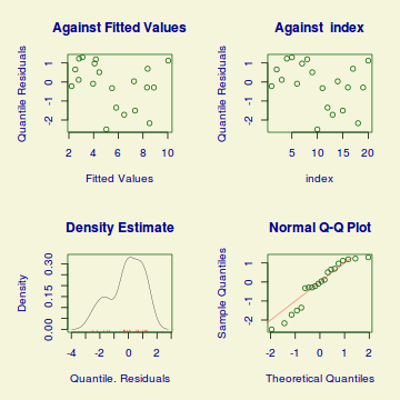
*******************************************************************
	 Summary of the Randomised Quantile Residuals
                           mean   =  -0.1289
                       variance   =  1.37
               coef. of skewness  =  -0.5522
               coef. of kurtosis  =  2.037
Filliben correlation coefficient  =  0.9624
*******************************************************************
In this demonstration we fitted two ZIP models. We could compare the fit of each of these zero-inflated poisson models to that of a regular Poisson model (that assumes a dispersion of 1 and no excessive zeros), using AIC.
Conclusions: The AIC is substantially smaller for the zero-inflated poisson models than the standard Poisson regression model. Hence we would conclude that the zero-inflated models are a better fit than the Poisson regression model.> dat.glm <- glm(y ~ x, data = dat.zip, family = "poisson") > AIC(dat.zeroinfl, dat.gamlss, dat.glm)
             df    AIC
dat.zeroinfl  3  78.34
dat.gamlss    3  78.34
dat.glm       2 124.01
Exploring the model parameters, test hypotheses
If there was any evidence that the assumptions had been violated or the model was not an appropriate fit, then we would need to reconsider the model and start the process again. In this case, there is no evidence that the test will be unreliable so we can proceed to explore the test statistics. The main statistic of interest is the Wald statistic ($z$) for the zeroinfl model and the t-statistic ($t$) for the gamlss model. The analyses are partitioned into the binary and Poisson components. For the Poisson component, it is the slope parameter that is of the primary interest. Since the models specified that the binomial component was to be modeled only against an intercept, the binomial output includes only an estimate for the intercept.
- zeroinfl
> summary(dat.zeroinfl)
Call: zeroinfl(formula = y ~ x | 1, data = dat.zip, dist = "poisson") Pearson residuals: Min 1Q Median 3Q Max -1.001 -0.956 -0.393 0.966 1.619 Count model coefficients (poisson with log link): Estimate Std. Error z value Pr(>|z|) (Intercept) 0.7047 0.3196 2.21 0.02745 * x 0.0873 0.0253 3.45 0.00056 *** Zero-inflation model coefficients (binomial with logit link): Estimate Std. Error z value Pr(>|z|) (Intercept) -0.229 0.456 -0.5 0.62 --- Signif. codes: 0 '***' 0.001 '**' 0.01 '*' 0.05 '.' 0.1 ' ' 1 Number of iterations in BFGS optimization: 13 Log-likelihood: -36.2 on 3 Df - gamlss
> summary(dat.gamlss)
*******************************************************************
Family:  c("ZIP", "Poisson Zero Inflated")

Call:  gamlss(formula = y ~ x, family = ZIP, data = dat.zip)

Fitting method: RS()

-------------------------------------------------------------------
Mu link function:  log
Mu Coefficients:
             Estimate  Std. Error  t value  Pr(>|t|)
(Intercept)    0.7058      0.3196     2.21   0.04123
x              0.0872      0.0253     3.44   0.00311

-------------------------------------------------------------------
Sigma link function:  logit
Sigma Coefficients:
  Estimate  Std. Error     t value    Pr(>|t|)
    -0.229       0.456      -0.502       0.622

-------------------------------------------------------------------
No. of observations in the fit:  20
Degrees of Freedom for the fit:  3
      Residual Deg. of Freedom:  17
                      at cycle:  3

Global Deviance:     72.34
            AIC:     78.34
            SBC:     81.33
*******************************************************************
Conclusions: We would reject the null hypothesis (p<0.05) from each model. Note that the two different approaches adopt a differnet reference distribution. Whilst zeroinf uses the Wald statistic ($z$), gamlss uses the t-statistic ($t$). An increase in x is associated with a significant linear increase (positive slope) in log $y$ abundance. Every 1 unit increase in $x$ is associated with a 0.087 unit increase in $\log y$ abundance We usually express this in terms of $y$ than $\log y$, so every 1 unit increase in $x$ is associated with a ($e^{0.087}=1.09$) 1.09 unit increase in $y$ abundance.
Further explorations of the trends
Now for a summary plot.
> par(mar = c(4, 5, 0, 0))
> plot(y ~ x, data = dat.zip, type = "n", ann = F, axes = F)
> points(y ~ x, data = dat.zip, pch = 16)
> xs <- seq(min(dat.zip$x), max(dat.zip$x), l = 100)
> coefs <- coef(dat.zeroinfl, model = "count")
> mm <- model.matrix(~x, data = data.frame(x = xs))
> vcov <- vcov(dat.zeroinfl, model = "count")
> ys <- vector("list")
> ys$fit <- exp(mm %*% coefs)
> points(ys$fit ~ xs, col = "black", type = "l")
>
> ys$se.fit <- exp(sqrt(diag(mm %*% vcov %*% t(mm))))
> lines(ys$fit - 1 * ys$se.fit ~ xs, col = "black", type = "l", lty = 2)
> lines(ys$fit + 1 * ys$se.fit ~ xs, col = "black", type = "l", lty = 2)
> axis(1)
> mtext("X", 1, cex = 1.5, line = 3)
> axis(2, las = 2)
> mtext("Abundance of Y", 2, cex = 1.5, line = 3)
> box(bty = "l")

Log-linear models
Scenario and Data
- Deviance ($G^2$) - similar to the $\chi^2$ test above, yet uses deviance
