Tutorial 12.2a - Non-linear least squares regression

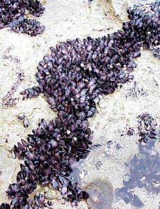
Peake and Quinn (1993) investigated the relationship between the size of mussel clumps (m²) and the number of other invertebrate species supported.

Download Peake data set

Format of peake.csv data file
AREA SPECIES INDIV 516.0 3 18 469.06 7 60 462.25 6 57 ... ... ... AREA Area of the mussel clump (m2)- predictor variable SPECIES Number of other invertebrate species found in the mussel clumps - response variable INDIV Number of other invertebrate individuals found in the mussel clumps - ignore this response variable

peake <- read.table('../downloads/data/peake.csv', header=T, sep=',', strip.white=T)
head(peake)

    AREA SPECIES INDIV
1  516.0       3    18
2  469.1       7    60
3  462.2       6    57
4  938.6       8   100
5 1357.2      10    48
6 1773.7       9   118

1. For this question we will focus on an examination of the relationship between the number of species occupying a mussel clump and the size of the mussel clump. Construct a scatterplot
   to investigate the assumptions of simple linear regression(HINT)
   Show code

   library(car)
   scatterplot(SPECIES~AREA,data=peake)
   

   
   1. Focussing on the assumptions of Normality, Homogeneity of Variance and Linearity, is there evidence of violations of these assumptions (y or n)?
2. Although we could try a logarithmic transformation of the AREA variable, species/area curves are known to be non-linear. We might expect that small clumps would only support a small number of species. However, as area increases, there should be a dramatic increase in the number of species supported. Finally, further increases in area should see the number of species approach an asymptote. Species-area data are often modeled with non-linear functions:
   1. Try fitting a second order polynomial trendline
      through these data. E.g. Species = α*Area + β*Area² + c (note that this is just an extension of y=mx+c)
      Show code

      peake.lm <- lm(SPECIES~AREA+I(AREA^2), data=peake)
      

   2. Try fitting a power trendline
      through these data. E.g. Species = α(Area)^β where the number of Species is proportional to the Area to the power of some coefficient (β).
      Show code

      peake.nls <- nls(SPECIES~alpha*AREA^beta, data=peake, start=list(alpha=0.1,beta=1))
      

   3. Try fitting an asymptotic exponential relationship through these data. E.g. Species = α-βe^γArea.
      Show code

      peake.nls1 <- nls(SPECIES~SSasymp(AREA,a,b,c),data=peake)
      

3. Compare the fit (via AIC, MSresidual and ANOVA) of each of the alternatives (also include the regular linear regression model).
   Show code

   peake.lmLin <- lm(SPECIES~AREA, data=peake)
   #calculate AIC for the linear model
   AIC(peake.lmLin)
   

   [1] 141.1
   

   # calculate mean-square residual of the linear model
   deviance(peake.lmLin)/df.residual(peake.lmLin)
   

   [1] 14.13
   

   AIC(peake.lm)
   

   [1] 129.5
   

   # calculate mean-square residual of the power model
   deviance(peake.lm)/df.residual(peake.lm)
   

   [1] 8.602
   

   # assess the goodness of fit between linear and polynomial models
   anova(peake.lmLin, peake.lm)
   

   Analysis of Variance Table
   
   Model 1: SPECIES ~ AREA
   Model 2: SPECIES ~ AREA + I(AREA^2)
     Res.Df RSS Df Sum of Sq    F  Pr(>F)    
   1     23 325                              
   2     22 189  1       136 15.8 0.00064 ***
   ---
   Signif. codes:  
   0 '***' 0.001 '**' 0.01 '*' 0.05 '.' 0.1 ' ' 1
   

   #calculate AIC for the exponential asymptotic model
   AIC(peake.nls)
   

   [1] 125.1
   

   # calculate mean-square residual of the exponential asymptotic model
   deviance(peake.nls)/df.residual(peake.nls)
   

   [1] 7.469
   

   #calculate AIC for the exponential asymptotic model
   AIC(peake.nls1)
   

   [1] 125.8
   

   # calculate mean-square residual of the exponential asymptotic model
   deviance(peake.nls1)/df.residual(peake.nls1)
   

   [1] 7.393
   

   # assess the goodness of fit between polynomial and power models
   anova(peake.nls, peake.nls1)
   

   Analysis of Variance Table
   
   Model 1: SPECIES ~ alpha * AREA^beta
   Model 2: SPECIES ~ SSasymp(AREA, a, b, c)
     Res.Df Res.Sum Sq Df Sum Sq F value Pr(>F)
   1     23        172                         
   2     22        163  1   9.14    1.24   0.28
   

   Model	AIC	MSresid	P-value
   Species = β*Area + c			Compare linear and polynomial in the box below
   Species = α*Area + β*Area2 + c
   Species = α(Area)β			Compare power and asymptotic exponential in the box below
   Species = α-βeγArea

Selecting the most appropriate model to relate the number of species to mussel clump area now becomes a combination of both inferential signals and theoretical biology/ecology. Our knowledge of biology tells us that it is nonsense to suggest that continual mussel clump size increases will result in further linear increases in the number of species encountered. Whilst it is possible that species numbers could reach an maximum at an optimum clump area, the polynomial fit (whilst empirically better than a linear fit - lower AIC and MSresid), is only marginally more suitable. The power and asymptotic exponential models both fit the data substantially (significantly?? - some argue that AIC values 2 units lower are significantly lower) better than either of the linear models. The two non-linear models were not found to differ significantly from one another (in terms of ANOVA or AIC), yet arguably the exponential model that indicates the species numbers rise faster before eventually plateauing off might be considered a more realistic model.

4. Create a plot of species number against mussel clump area. Actually, this might be a good point to plot each of the competing models on separate sub-figures. Hence we will go through the process of building up the four sub-figures in a grid in the one larger figure.
   1. Start by setting up some whole figure (graphics device) parameters. In particular, indicate that the overall figure is going to comprise 2 rows and 2 columns.
      Show code

      opar<-par(mfrow=c(2,2))
      

   2. Setup the margins (5 units on the bottom and left and 0 units on the top and right) and dimensions of the blank plotting space. Also add the raw observations as solid grey dots
      Show code

      #first plot linear trend
      opar1 <- par(mar=c(5,5,0,0))
      plot(SPECIES~AREA, data=peake, ann=F, axes=F, type="n")
      points(SPECIES~AREA, data=peake,col="grey", pch=16)
      

      
   3. Use the predict function to generate predicted (fitted) values and 95% confidence intervals for 1000 new AREA values between the minimum and maximum original AREA range. Plot the trend and confidence intervals in solid and dotted lines respectively.
      Show code

      xs<-with(peake,seq(min(AREA),max(AREA),l=1000))
      ys <- predict(peake.lmLin, data.frame(AREA=xs), interval="confidence")
      points(ys[,'fit']~xs,col="black", type="l")
      

      
   4. Add axes, axes titles and a "L" shape axes box to the plot to complete the first sub-figure
      Show code

      ys <- predict(peake.lmLin, data.frame(AREA=xs), interval="confidence")
      points(ys[,'fit']~xs,col="black", type="l")
      points(ys[,'lwr']~xs,col="black", type="l",lty=2)
      points(ys[,'upr']~xs,col="black", type="l",lty=2)
      axis(1,cex.axis=0.75)
      mtext(expression(paste("Clump area",(dm^2))),1,line=3, cex=1.2)
      axis(2,las=1,cex.axis=0.75)
      mtext(expression(paste("Number of species (",phantom()%+-%95,"%CI)")),2,line=3, cex=1.2)
      box(bty="l")
      par(opar1)
      

      
   5. Complete the second sub-figure (polynomial trend) in much the same manner as the first (linear trend)
      Show code

      opar <- par(mfrow=c(2,2))
      #first plot linear trend
      opar1 <- par(mar=c(5,5,0,0))
      plot(SPECIES~AREA, data=peake, ann=F, axes=F, type="n")
      points(SPECIES~AREA, data=peake,col="grey", pch=16)
      xs<-with(peake,seq(min(AREA),max(AREA),l=1000))
      ys <- predict(peake.lmLin, data.frame(AREA=xs), interval="confidence")
      points(ys[,'fit']~xs,col="black", type="l")
      points(ys[,'lwr']~xs,col="black", type="l",lty=2)
      points(ys[,'upr']~xs,col="black", type="l",lty=2)
      axis(1,cex.axis=0.75)
      mtext(expression(paste("Clump area",(dm^2))),1,line=3, cex=1.2)
      axis(2,las=1,cex.axis=0.75)
      mtext(expression(paste("Number of species (",phantom()%+-%95,"%CI)")),2,line=3, cex=1.2)
      box(bty="l")
      par(opar1)
      #second plot polynomial trend
      opar1 <- par(mar=c(5,5,0,0))
      plot(SPECIES~AREA, data=peake, ann=F, axes=F, type="n")
      points(SPECIES~AREA, data=peake,col="grey", pch=16)
      xs<-with(peake,seq(min(AREA),max(AREA),l=1000))
      ys <- predict(peake.lm, data.frame(AREA=xs), interval="confidence")
      points(ys[,'fit']~xs,col="black", type="l")
      points(ys[,'lwr']~xs,col="black", type="l",lty=2)
      points(ys[,'upr']~xs,col="black", type="l",lty=2)
      axis(1,cex.axis=0.75)
      mtext(expression(paste("Clump area",(dm^2))),1,line=3, cex=1.2)
      axis(2,las=1,cex.axis=0.75)
      mtext(expression(paste("Number of species (",phantom()%+-%95,"%CI)")),2,line=3, cex=1.2)
      box(bty="l")
      par(opar1)
      

      
   6. Start the third (power) model similarly
      Show code

      opar <- par(mfrow=c(2,2))
      #first plot linear trend
      opar1 <- par(mar=c(5,5,0,0))
      plot(SPECIES~AREA, data=peake, ann=F, axes=F, type="n")
      points(SPECIES~AREA, data=peake,col="grey", pch=16)
      xs<-with(peake,seq(min(AREA),max(AREA),l=1000))
      ys <- predict(peake.lmLin, data.frame(AREA=xs), interval="confidence")
      points(ys[,'fit']~xs,col="black", type="l")
      points(ys[,'lwr']~xs,col="black", type="l",lty=2)
      points(ys[,'upr']~xs,col="black", type="l",lty=2)
      axis(1,cex.axis=0.75)
      mtext(expression(paste("Clump area",(dm^2))),1,line=3, cex=1.2)
      axis(2,las=1,cex.axis=0.75)
      mtext(expression(paste("Number of species (",phantom()%+-%95,"%CI)")),2,line=3, cex=1.2)
      box(bty="l")
      par(opar1)
      #second plot polynomial trend
      opar1 <- par(mar=c(5,5,0,0))
      plot(SPECIES~AREA, data=peake, ann=F, axes=F, type="n")
      points(SPECIES~AREA, data=peake,col="grey", pch=16)
      xs<-with(peake,seq(min(AREA),max(AREA),l=1000))
      ys <- predict(peake.lm, data.frame(AREA=xs), interval="confidence")
      points(ys[,'fit']~xs,col="black", type="l")
      points(ys[,'lwr']~xs,col="black", type="l",lty=2)
      points(ys[,'upr']~xs,col="black", type="l",lty=2)
      axis(1,cex.axis=0.75)
      mtext(expression(paste("Clump area",(dm^2))),1,line=3, cex=1.2)
      axis(2,las=1,cex.axis=0.75)
      mtext(expression(paste("Number of species (",phantom()%+-%95,"%CI)")),2,line=3, cex=1.2)
      box(bty="l")
      par(opar1)
      

      
   7. Estimating confidence intervals is a little more complex for non-linear least squares models as the predict() function does not yet support calculating standard errors or intervals. Nevertheless, we can do this manually (go R you good thing!).
      1. Firstly we need to refit the non-linear power model incorporating a function that will be used to specify gradient calculations. This will be necessary to form the basis of SE calculations. So the gradient needs to be specified using the deriv3() function.
      2. Secondly, we then refit the power model using this new gradient function
      Show code

      opar <- par(mfrow=c(2,2))
      #first plot linear trend
      opar1 <- par(mar=c(5,5,0,0))
      plot(SPECIES~AREA, data=peake, ann=F, axes=F, type="n")
      points(SPECIES~AREA, data=peake,col="grey", pch=16)
      xs<-with(peake,seq(min(AREA),max(AREA),l=1000))
      ys <- predict(peake.lmLin, data.frame(AREA=xs), interval="confidence")
      points(ys[,'fit']~xs,col="black", type="l")
      points(ys[,'lwr']~xs,col="black", type="l",lty=2)
      points(ys[,'upr']~xs,col="black", type="l",lty=2)
      axis(1,cex.axis=0.75)
      mtext(expression(paste("Clump area",(dm^2))),1,line=3, cex=1.2)
      axis(2,las=1,cex.axis=0.75)
      mtext(expression(paste("Number of species (",phantom()%+-%95,"%CI)")),2,line=3, cex=1.2)
      box(bty="l")
      par(opar1)
      #second plot polynomial trend
      opar1 <- par(mar=c(5,5,0,0))
      plot(SPECIES~AREA, data=peake, ann=F, axes=F, type="n")
      points(SPECIES~AREA, data=peake,col="grey", pch=16)
      xs<-with(peake,seq(min(AREA),max(AREA),l=1000))
      ys <- predict(peake.lm, data.frame(AREA=xs), interval="confidence")
      points(ys[,'fit']~xs,col="black", type="l")
      points(ys[,'lwr']~xs,col="black", type="l",lty=2)
      points(ys[,'upr']~xs,col="black", type="l",lty=2)
      axis(1,cex.axis=0.75)
      mtext(expression(paste("Clump area",(dm^2))),1,line=3, cex=1.2)
      axis(2,las=1,cex.axis=0.75)
      mtext(expression(paste("Number of species (",phantom()%+-%95,"%CI)")),2,line=3, cex=1.2)
      box(bty="l")
      par(opar1)
      #we need to refit the model in order to get gradient calculations from which se can be calculated
      # this requires that the gradient be specified using the deriv3() function.
      grad <- deriv3(~alpha*AREA^beta, c("alpha","beta"), function(alpha,beta,AREA) NULL)
      peake.nls<-nls(SPECIES~grad(alpha,beta,AREA), data=peake,start=list(alpha=0.1,beta=1))
      

      
   8. The predicted values of the trend as well as standard errors can then be calculated and used to plot approximate 95% confidence intervals. One standard error is equivalent to approximately 68% confidence intervals. The conversion between standard error and 95% confidence interval follows the formula 95%CI=1.96xSE. Actually, 1.96 (or 2) is an approximation from large (>30) sample sizes. A more exact solution can be obtained by multiplying the SE by pt(0.975,df) where df is the degrees of freedom.
      Show code

      opar <- par(mfrow=c(2,2))
      #first plot linear trend
      opar1 <- par(mar=c(5,5,0,0))
      plot(SPECIES~AREA, data=peake, ann=F, axes=F, type="n")
      points(SPECIES~AREA, data=peake,col="grey", pch=16)
      xs<-with(peake,seq(min(AREA),max(AREA),l=1000))
      ys <- predict(peake.lmLin, data.frame(AREA=xs), interval="confidence")
      points(ys[,'fit']~xs,col="black", type="l")
      points(ys[,'lwr']~xs,col="black", type="l",lty=2)
      points(ys[,'upr']~xs,col="black", type="l",lty=2)
      axis(1,cex.axis=0.75)
      mtext(expression(paste("Clump area",(dm^2))),1,line=3, cex=1.2)
      axis(2,las=1,cex.axis=0.75)
      mtext(expression(paste("Number of species (",phantom()%+-%95,"%CI)")),2,line=3, cex=1.2)
      box(bty="l")
      par(opar1)
      #second plot polynomial trend
      opar1 <- par(mar=c(5,5,0,0))
      plot(SPECIES~AREA, data=peake, ann=F, axes=F, type="n")
      points(SPECIES~AREA, data=peake,col="grey", pch=16)
      xs<-with(peake,seq(min(AREA),max(AREA),l=1000))
      ys <- predict(peake.lm, data.frame(AREA=xs), interval="confidence")
      points(ys[,'fit']~xs,col="black", type="l")
      points(ys[,'lwr']~xs,col="black", type="l",lty=2)
      points(ys[,'upr']~xs,col="black", type="l",lty=2)
      axis(1,cex.axis=0.75)
      mtext(expression(paste("Clump area",(dm^2))),1,line=3, cex=1.2)
      axis(2,las=1,cex.axis=0.75)
      mtext(expression(paste("Number of species (",phantom()%+-%95,"%CI)")),2,line=3, cex=1.2)
      box(bty="l")
      par(opar1)
      #we need to refit the model in order to get gradient calculations from which se can be calculated
      # this requires that the gradient be specified using the deriv3() function.
      grad <- deriv3(~alpha*AREA^beta, c("alpha","beta"), function(alpha,beta,AREA) NULL)
      peake.nls<-nls(SPECIES~grad(alpha,beta,AREA), data=peake,start=list(alpha=0.1,beta=1))
      ys <- predict(peake.nls, data.frame(AREA=xs))
      se.fit <- sqrt(apply(attr(predict(peake.nls1,list(AREA = xs)),"gradient"),1,function(x) sum(vcov(peake.nls1)*outer(x,x))))
      opar1 <- par(mar=c(5,5,0,0))
      plot(SPECIES~AREA, data=peake, ann=F, axes=F, type="n")
      points(ys~xs,col="black", type="l")
      #2*SE equates approximately to 95% confidence intervals
      #technically it is qt(0.975,df)*SE
      #therefore this could also be labeled as 90%CI
      points(ys+2*se.fit~xs,col="black", type="l",lty=2)
      points(ys-2*se.fit~xs,col="black", type="l",lty=2)
      

      
   9. Finish sub-figure 3 similar to the other two
      Show code

      opar <- par(mfrow=c(2,2))
      #first plot linear trend
      opar1 <- par(mar=c(5,5,0,0))
      plot(SPECIES~AREA, data=peake, ann=F, axes=F, type="n")
      points(SPECIES~AREA, data=peake,col="grey", pch=16)
      xs<-with(peake,seq(min(AREA),max(AREA),l=1000))
      ys <- predict(peake.lmLin, data.frame(AREA=xs), interval="confidence")
      points(ys[,'fit']~xs,col="black", type="l")
      points(ys[,'lwr']~xs,col="black", type="l",lty=2)
      points(ys[,'upr']~xs,col="black", type="l",lty=2)
      axis(1,cex.axis=0.75)
      mtext(expression(paste("Clump area",(dm^2))),1,line=3, cex=1.2)
      axis(2,las=1,cex.axis=0.75)
      mtext(expression(paste("Number of species (",phantom()%+-%95,"%CI)")),2,line=3, cex=1.2)
      box(bty="l")
      par(opar1)
      #second plot polynomial trend
      opar1 <- par(mar=c(5,5,0,0))
      plot(SPECIES~AREA, data=peake, ann=F, axes=F, type="n")
      points(SPECIES~AREA, data=peake,col="grey", pch=16)
      xs<-with(peake,seq(min(AREA),max(AREA),l=1000))
      ys <- predict(peake.lm, data.frame(AREA=xs), interval="confidence")
      points(ys[,'fit']~xs,col="black", type="l")
      points(ys[,'lwr']~xs,col="black", type="l",lty=2)
      points(ys[,'upr']~xs,col="black", type="l",lty=2)
      axis(1,cex.axis=0.75)
      mtext(expression(paste("Clump area",(dm^2))),1,line=3, cex=1.2)
      axis(2,las=1,cex.axis=0.75)
      mtext(expression(paste("Number of species (",phantom()%+-%95,"%CI)")),2,line=3, cex=1.2)
      box(bty="l")
      par(opar1)
      #we need to refit the model in order to get gradient calculations from which se can be calculated
      # this requires that the gradient be specified using the deriv3() function.
      grad <- deriv3(~alpha*AREA^beta, c("alpha","beta"), function(alpha,beta,AREA) NULL)
      peake.nls<-nls(SPECIES~grad(alpha,beta,AREA), data=peake,start=list(alpha=0.1,beta=1))
      ys <- predict(peake.nls, data.frame(AREA=xs))
      se.fit <- sqrt(apply(attr(predict(peake.nls1,list(AREA = xs)),"gradient"),1,function(x) sum(vcov(peake.nls1)*outer(x,x))))
      opar1 <- par(mar=c(5,5,0,0))
      plot(SPECIES~AREA, data=peake, ann=F, axes=F, type="n")
      points(ys~xs,col="black", type="l")
      #2*SE equates approximately to 95% confidence intervals
      #technically it is qt(0.975,df)*SE
      #therefore this could also be labeled as 90%CI
      points(ys+2*se.fit~xs,col="black", type="l",lty=2)
      points(ys-2*se.fit~xs,col="black", type="l",lty=2)
      points(ys+2*se.fit~xs,col="black", type="l",lty=2)
      points(ys-2*se.fit~xs,col="black", type="l",lty=2)
      axis(1,cex.axis=0.75)
      mtext(expression(paste("Clump area",(dm^2))),1,line=3, cex=1.2)
      axis(2,las=1,cex.axis=0.75)
      mtext(expression(paste("Number of species",(phantom()%+-%2~SE),)),2,line=3, cex=1.2)
      box(bty="l")
      par(opar1)
      

      
   10. Sub-figure four (asymptotic exponential) is similar to the power model except that as it already incorporates a gradient function (SSasymp()), this step is not required.
       Show code

       opar <- par(mfrow=c(2,2))
       #first plot linear trend
       opar1 <- par(mar=c(5,5,0,0))
       plot(SPECIES~AREA, data=peake, ann=F, axes=F, type="n")
       points(SPECIES~AREA, data=peake,col="grey", pch=16)
       xs<-with(peake,seq(min(AREA),max(AREA),l=1000))
       ys <- predict(peake.lmLin, data.frame(AREA=xs), interval="confidence")
       points(ys[,'fit']~xs,col="black", type="l")
       points(ys[,'lwr']~xs,col="black", type="l",lty=2)
       points(ys[,'upr']~xs,col="black", type="l",lty=2)
       axis(1,cex.axis=0.75)
       mtext(expression(paste("Clump area",(dm^2))),1,line=3, cex=1.2)
       axis(2,las=1,cex.axis=0.75)
       mtext(expression(paste("Number of species (",phantom()%+-%95,"%CI)")),2,line=3, cex=1.2)
       box(bty="l")
       par(opar1)
       #second plot polynomial trend
       opar1 <- par(mar=c(5,5,0,0))
       plot(SPECIES~AREA, data=peake, ann=F, axes=F, type="n")
       points(SPECIES~AREA, data=peake,col="grey", pch=16)
       xs<-with(peake,seq(min(AREA),max(AREA),l=1000))
       ys <- predict(peake.lm, data.frame(AREA=xs), interval="confidence")
       points(ys[,'fit']~xs,col="black", type="l")
       points(ys[,'lwr']~xs,col="black", type="l",lty=2)
       points(ys[,'upr']~xs,col="black", type="l",lty=2)
       axis(1,cex.axis=0.75)
       mtext(expression(paste("Clump area",(dm^2))),1,line=3, cex=1.2)
       axis(2,las=1,cex.axis=0.75)
       mtext(expression(paste("Number of species (",phantom()%+-%95,"%CI)")),2,line=3, cex=1.2)
       box(bty="l")
       par(opar1)
       #we need to refit the model in order to get gradient calculations from which se can be calculated
       # this requires that the gradient be specified using the deriv3() function.
       grad <- deriv3(~alpha*AREA^beta, c("alpha","beta"), function(alpha,beta,AREA) NULL)
       peake.nls<-nls(SPECIES~grad(alpha,beta,AREA), data=peake,start=list(alpha=0.1,beta=1))
       ys <- predict(peake.nls, data.frame(AREA=xs))
       se.fit <- sqrt(apply(attr(predict(peake.nls1,list(AREA = xs)),"gradient"),1,function(x) sum(vcov(peake.nls1)*outer(x,x))))
       opar1 <- par(mar=c(5,5,0,0))
       plot(SPECIES~AREA, data=peake, ann=F, axes=F, type="n")
       points(ys~xs,col="black", type="l")
       #2*SE equates approximately to 95% confidence intervals
       #technically it is qt(0.975,df)*SE
       #therefore this could also be labeled as 90%CI
       points(ys+2*se.fit~xs,col="black", type="l",lty=2)
       points(ys-2*se.fit~xs,col="black", type="l",lty=2)
       points(ys+2*se.fit~xs,col="black", type="l",lty=2)
       points(ys-2*se.fit~xs,col="black", type="l",lty=2)
       axis(1,cex.axis=0.75)
       mtext(expression(paste("Clump area",(dm^2))),1,line=3, cex=1.2)
       axis(2,las=1,cex.axis=0.75)
       mtext(expression(paste("Number of species",(phantom()%+-%2~SE),)),2,line=3, cex=1.2)
       box(bty="l")
       par(opar1)
       #forth plot trend with standard error
       opar1 <- par(mar=c(5,5,0,0))
       plot(SPECIES~AREA, data=peake, ann=F, axes=F, type="n")
       points(SPECIES~AREA, data=peake,col="grey", pch=16)
       xs<-with(peake,seq(min(AREA),max(AREA),l=1000))
       ys <- predict(peake.nls1, data.frame(AREA=xs))
       se.fit <- sqrt(apply(attr(ys,"gradient"),1,function(x) sum(vcov(peake.nls1)*outer(x,x))))
       points(ys~xs,col="black", type="l")
       points(ys+2*se.fit~xs,col="black", type="l",lty=2)
       points(ys-2*se.fit~xs,col="black", type="l",lty=2)
       axis(1,cex.axis=0.75)
       mtext(expression(paste("Clump area",(dm^2))),1,line=3, cex=1.2)
       axis(2,las=1,cex.axis=0.75)
       mtext(expression(paste("Number of species",(phantom()%+-%2~SE),)),2,line=3, cex=1.2)
       box(bty="l")
       

       

       par(opar1)
       

   11. Finally, finalize the figure by restoring the plotting (graphics device) parameters
       Show code

       opar <- par(mfrow=c(2,2))
       #first plot linear trend
       opar1 <- par(mar=c(5,5,0,0))
       plot(SPECIES~AREA, data=peake, ann=F, axes=F, type="n")
       points(SPECIES~AREA, data=peake,col="grey", pch=16)
       xs<-with(peake,seq(min(AREA),max(AREA),l=1000))
       ys <- predict(peake.lmLin, data.frame(AREA=xs), interval="confidence")
       points(ys[,'fit']~xs,col="black", type="l")
       points(ys[,'lwr']~xs,col="black", type="l",lty=2)
       points(ys[,'upr']~xs,col="black", type="l",lty=2)
       axis(1,cex.axis=0.75)
       mtext(expression(paste("Clump area",(dm^2))),1,line=3, cex=1.2)
       axis(2,las=1,cex.axis=0.75)
       mtext(expression(paste("Number of species (",phantom()%+-%95,"%CI)")),2,line=3, cex=1.2)
       box(bty="l")
       par(opar1)
       #second plot polynomial trend
       opar1 <- par(mar=c(5,5,0,0))
       plot(SPECIES~AREA, data=peake, ann=F, axes=F, type="n")
       points(SPECIES~AREA, data=peake,col="grey", pch=16)
       xs<-with(peake,seq(min(AREA),max(AREA),l=1000))
       ys <- predict(peake.lm, data.frame(AREA=xs), interval="confidence")
       points(ys[,'fit']~xs,col="black", type="l")
       points(ys[,'lwr']~xs,col="black", type="l",lty=2)
       points(ys[,'upr']~xs,col="black", type="l",lty=2)
       axis(1,cex.axis=0.75)
       mtext(expression(paste("Clump area",(dm^2))),1,line=3, cex=1.2)
       axis(2,las=1,cex.axis=0.75)
       mtext(expression(paste("Number of species (",phantom()%+-%95,"%CI)")),2,line=3, cex=1.2)
       box(bty="l")
       par(opar1)
       #we need to refit the model in order to get gradient calculations from which se can be calculated
       # this requires that the gradient be specified using the deriv3() function.
       grad <- deriv3(~alpha*AREA^beta, c("alpha","beta"), function(alpha,beta,AREA) NULL)
       peake.nls<-nls(SPECIES~grad(alpha,beta,AREA), data=peake,start=list(alpha=0.1,beta=1))
       ys <- predict(peake.nls, data.frame(AREA=xs))
       se.fit <- sqrt(apply(attr(predict(peake.nls1,list(AREA = xs)),"gradient"),1,function(x) sum(vcov(peake.nls1)*outer(x,x))))
       opar1 <- par(mar=c(5,5,0,0))
       plot(SPECIES~AREA, data=peake, ann=F, axes=F, type="n")
       points(ys~xs,col="black", type="l")
       #2*SE equates approximately to 95% confidence intervals
       #technically it is qt(0.975,df)*SE
       #therefore this could also be labeled as 90%CI
       points(ys+2*se.fit~xs,col="black", type="l",lty=2)
       points(ys-2*se.fit~xs,col="black", type="l",lty=2)
       points(ys+2*se.fit~xs,col="black", type="l",lty=2)
       points(ys-2*se.fit~xs,col="black", type="l",lty=2)
       axis(1,cex.axis=0.75)
       mtext(expression(paste("Clump area",(dm^2))),1,line=3, cex=1.2)
       axis(2,las=1,cex.axis=0.75)
       mtext(expression(paste("Number of species",(phantom()%+-%2~SE),)),2,line=3, cex=1.2)
       box(bty="l")
       par(opar1)
       #forth plot trend with standard error
       opar1 <- par(mar=c(5,5,0,0))
       plot(SPECIES~AREA, data=peake, ann=F, axes=F, type="n")
       points(SPECIES~AREA, data=peake,col="grey", pch=16)
       xs<-with(peake,seq(min(AREA),max(AREA),l=1000))
       ys <- predict(peake.nls1, data.frame(AREA=xs))
       se.fit <- sqrt(apply(attr(ys,"gradient"),1,function(x) sum(vcov(peake.nls1)*outer(x,x))))
       points(ys~xs,col="black", type="l")
       points(ys+2*se.fit~xs,col="black", type="l",lty=2)
       points(ys-2*se.fit~xs,col="black", type="l",lty=2)
       axis(1,cex.axis=0.75)
       mtext(expression(paste("Clump area",(dm^2))),1,line=3, cex=1.2)
       axis(2,las=1,cex.axis=0.75)
       mtext(expression(paste("Number of species",(phantom()%+-%2~SE),)),2,line=3, cex=1.2)
       box(bty="l")
       

       

       par(opar1)
       par(opar)