Tutorial 13.2 - Species richness and diversity
11 Mar 2015
> library(vegan)
> library(ggplot2)
> library(grid)
> #define my common ggplot options
> murray_opts <- opts(panel.grid.major=theme_blank(),
+                            panel.grid.minor=theme_blank(),
+                            panel.border = theme_blank(),
+                            panel.background = theme_blank(),
+                            axis.title.y=theme_text(size=15, vjust=0,angle=90),
+                            axis.text.y=theme_text(size=12),
+                            axis.title.x=theme_text(size=15, vjust=-1),
+                            axis.text.x=theme_text(size=12),
+                            axis.line = theme_segment(),
+                            plot.margin=unit(c(0.5,0.5,1,2),"lines")
+ )
Error: Use 'theme' instead. (Defunct;
last used in version 0.9.1)
> coenocline <- function(x,A0,m,r,a,g, int=T, noise=T) {
+ #x is the environmental range
+ #A0 is the maximum abundance of the species at the optimum environmental conditions
+ #m is the value of the environmental gradient that represents the optimum conditions for the species
+ #r the species range over the environmental gradient (niche width)
+ #a and g are shape parameters representing the skewness and kurtosis
+ # when a=g, the distribution is symmetrical
+ # when a>g - negative skew (large left tail)
+ # when a<g - positive skew (large right tail)
+ #int - indicates whether the responses should be rounded to integers (=T)
+ #noise - indicates whether or not random noise should be added (reflecting random sampling)
+ #NOTE.  negative numbers converted to 0
+          b <- a/(a+g)
+          d <- (b^a)*(1-b)^g
+          cc <- (A0/d)*((((x-m)/r)+b)^a)*((1-(((x-m)/r)+b))^g)
+          if (noise) {n <- A0/10; n[n<0]<-0; cc<-cc+rnorm(length(cc),0,n)}
+          cc[cc<0] <- 0
+          cc[is.na(cc)]<-0
+          if (int) cc<-round(cc,0)
+          cc
+ }
> #plot(coenocline(0:100,40,40,20,1,1, int=T, noise=T), ylim=c(0,100))
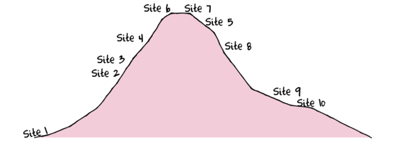
As with the other tutorials, we will use a simulated data set for this tutorial. This simulated data set comprises the abundances of 10 species within 10 sites located along a transect that extends in a northerly direction over a mountain range
> set.seed(1)
> x <- seq(0,50,l=10)
> n <- 10
> sp1<-coenocline(x=x,A0=5,m=0,r=2,a=1,g=1,int=T, noise=T)
> sp2<-coenocline(x=x,A0=70,m=7,r=30,a=1,g=1,int=T, noise=T)
> sp3<-coenocline(x=x,A0=50,m=15,r=30,a=1,g=1,int=T, noise=T)
> sp4<-coenocline(x=x,A0=7,m=25,r=20,a=0.4,g=0.1,int=T, noise=T)
> sp5<-coenocline(x=x,A0=40,m=30,r=30,a=0.6,g=0.5,int=T, noise=T)
> sp6<-coenocline(x=x,A0=15,m=35,r=15,a=0.2,g=0.3,int=T, noise=T)
> sp7<-coenocline(x=x,A0=20,m=45,r=25,a=0.5,g=0.9,int=T, noise=T)
> sp8<-coenocline(x=x,A0=5,m=45,r=5,a=1,g=1,int=T, noise=T)
> sp9<-coenocline(x=x,A0=20,m=45,r=15,a=1,g=1,int=T, noise=T)
> sp10<-coenocline(x=x,A0=30,m=50,r=5,a=1,g=1,int=T, noise=T)
> X <- cbind(sp1, sp10,sp9,sp2,sp3,sp8,sp4,sp5,sp7,sp6)
> #X<-X[c(1,10,9,2,3,8,4,5,7,6),]
> colnames(X) <- paste("Sp",1:10,sep="")
> rownames(X) <- paste("Site", c(1,10,9,2,3,8,4,5,7,6), sep="")
> X <- X[c(1,4,5,7,8,10,9,6,3,2),]
> data <- data.frame(Sites=factor(rownames(X),levels=rownames(X)), X)
| Sites | Sp1 | Sp2 | Sp3 | Sp4 | Sp5 | Sp6 | Sp7 | Sp8 | Sp9 | Sp10 |
|---|---|---|---|---|---|---|---|---|---|---|
| Site1 | 5 | 0 | 0 | 65 | 5 | 0 | 0 | 0 | 0 | 0 |
| Site2 | 0 | 0 | 0 | 25 | 39 | 0 | 6 | 23 | 0 | 0 |
| Site3 | 0 | 0 | 0 | 6 | 42 | 0 | 6 | 31 | 0 | 0 |
| Site4 | 0 | 0 | 0 | 0 | 0 | 0 | 0 | 40 | 0 | 14 |
| Site5 | 0 | 0 | 6 | 0 | 0 | 0 | 0 | 34 | 18 | 12 |
| Site6 | 0 | 29 | 12 | 0 | 0 | 0 | 0 | 0 | 22 | 0 |
| Site7 | 0 | 0 | 21 | 0 | 0 | 5 | 0 | 0 | 20 | 0 |
| Site8 | 0 | 0 | 0 | 0 | 13 | 0 | 6 | 37 | 0 | 0 |
| Site9 | 0 | 0 | 0 | 60 | 47 | 0 | 4 | 0 | 0 | 0 |
| Site10 | 0 | 0 | 0 | 72 | 34 | 0 | 0 | 0 | 0 | 0 |
Species richness
Species richness is a measure of the number of species (or other taxonomic level) present at a site. Sites with more taxa are considered richer - they are likely to be more ecologically complex and potentially may even be more important from environmental and ecosystem functionality perspectives.
The simplest measure of species richness is just the number of species recorded per site. That is, the number of species that have more than one individual recorded.
> # sum up the number of non-zero entries per row (1)
> # the first column is ignored [,-1] as it is a site name, not a species count.
> apply(data[,-1]>0,1,sum)
 Site1  Site2  Site3  Site4  Site5
     3      4      4      2      4
 Site6  Site7  Site8  Site9 Site10
     3      3      3      3      2
> #OR
> library(plyr)
> ddply(data,~Sites,function(x) {
+   data.frame(RICHNESS=sum(x[-1]>0))
+ })
    Sites RICHNESS
1   Site1        3
2   Site2        4
3   Site3        4
4   Site4        2
5   Site5        4
6   Site6        3
7   Site7        3
8   Site8        3
9   Site9        3
10 Site10        2
When measuring richness (the number of species), we really should consider sampling effort. Clearly, the longer we search, the more species we are likely to encounter. This concept is encapsulated within a typical species richness curve (a form of species discovery or species accumulation) which plots the total number of detected species against the total number of individuals sampled (as the measure of effort).

Intially new species are encountered at a rapid rate, yet this eventually slows down to the point where each additional new species requires increasingly more effort. It is apparent in the above figure that there is relatively little benefit in sampling beyond 400 individuals.
There are numerous techniques that can be used to estimate the point at which the species richness curve would level off (asymptote) and therefore estimate species richness. Alternatively, species richness can be taken as the number of species detected before the rate of new detection falls below a threshold (such as 1%). Note that from the simulated data set, it is not possible to generate a species richness curve as we do not have the progressive build up of species and individual counts - only the final counts.
Nevertheless, there are a couple of indices that do take into account sample size:
- Menhinick's index is simply the number of species ($n$) divided by the square-root of the total number of individuals ($N$).
$$D=\frac{n}{\sqrt{N}}$$
> n<-apply(data[,-1]>0,1,sum)
> N <- apply(data[,-1],1,sum)
> n/sqrt(N)
 Site1  Site2  Site3  Site4  Site5
0.3464 0.4148 0.4339 0.2722 0.4781
 Site6  Site7  Site8  Site9 Site10
0.3780 0.4423 0.4009 0.2847 0.1943
> #OR
> library(plyr)
> menhinick <- function(x) {
+                          sum(x>0)/sqrt(sum(x))
+ }
> ddply(data,~Sites,function(x) {
+   data.frame(RICHNESS=menhinick(x[-1]))
+ })
    Sites RICHNESS
1   Site1   0.3464
2   Site2   0.4148
3   Site3   0.4339
4   Site4   0.2722
5   Site5   0.4781
6   Site6   0.3780
7   Site7   0.4423
8   Site8   0.4009
9   Site9   0.2847
10 Site10   0.1943
- Margalef's index is the number of species ($n$) minus 1 divided by the natural logarithm of the total number of individuals ($N$).
$$D=\frac{n-1}{ln N}$$
> n<-apply(data[,-1]>0,1,sum)
> N <- apply(data[,-1],1,sum)
> (n-1)/log(N)
 Site1  Site2  Site3  Site4  Site5
0.4632 0.6619 0.6753 0.2507 0.7061
 Site6  Site7  Site8  Site9 Site10
0.4827 0.5224 0.4969 0.4247 0.2144
> #OR
> library(plyr)
> menhinick <- function(x) {
+                          (sum(x>0)-1)/log(sum(x))
+ }
> ddply(data,~Sites,function(x) {
+   data.frame(RICHNESS=menhinick(x[-1]))
+ })
    Sites RICHNESS
1   Site1   0.4632
2   Site2   0.6619
3   Site3   0.6753
4   Site4   0.2507
5   Site5   0.7061
6   Site6   0.4827
7   Site7   0.5224
8   Site8   0.4969
9   Site9   0.4247
10 Site10   0.2144
Note however, species richness measures do not account for relative abundances within the different taxa. For example, the following two communities would be considered equivalent via each of the species richness indicies.
| Sp1 | Sp2 | Sp3 | Sp4 | Sp5 | |
|---|---|---|---|---|---|
| Site1 | 20 | 20 | 20 | 20 | 20 |
| Site2 | 96 | 1 | 1 | 1 | 1 |
- $n=5$
- $N=100$
- Menhinick's $D=0.5$
- Margalef's $D=0.866$
Species abundance and density
Another measure of a community is the total abundance of individuals present (per area).
> # sum up the number of non-zero entries per row (1)
> # the first column is ignored [,-1] as it is a site name, not a species count.
> apply(data[,-1],1,sum)
 Site1  Site2  Site3  Site4  Site5
    75     93     85     54     70
 Site6  Site7  Site8  Site9 Site10
    63     46     56    111    106
> #OR
> library(plyr)
> ddply(data,~Sites,function(x) {
+   data.frame(ABUNDANCE=sum(x[-1]))
+ })
    Sites ABUNDANCE
1   Site1        75
2   Site2        93
3   Site3        85
4   Site4        54
5   Site5        70
6   Site6        63
7   Site7        46
8   Site8        56
9   Site9       111
10 Site10       106
Simple species abundances are adequate if all species are collected using the same sampling technique or techniques that sample the same temporal and spatial scale. For example, some of the species might have individuals that are very large and thus detectable using a technique that covers a very wide area (such as aerial photography). Yet other species might be very small and require more intense searching and therefore require a more fine scale sampling unit (such as a quadrat). As it is not feasible to cover the same area with quadrats as with aerial photographs, it is necessary to standardize the counts for each species by expressing them per unit area.
With our fabricated data, let us assume that Species 1,2,5,7 and 9 were all small and were sampled from a total of 20 1x1m quadrats per site, whereas Species 2,4,6,8 and 10 were all very large and were sampled from a single 50x5m line transect per site. The densities per site expressed as the number per 1km2 would therefore be:
> data1 <- data
> data1[,c(2,4,6,8,10)] <- data1[,c(2,4,6,8,10)]*(1/20)
> data1[,c(3,5,7,9,11)] <- data1[,c(3,5,7,9,11)]*(1/250)
> apply(data1[,-1],1,sum)
 Site1  Site2  Site3  Site4  Site5
 0.760  2.442  2.548  0.216  1.384
 Site6  Site7  Site8  Site9 Site10
 1.816  2.070  1.098  2.790  1.988
> #OR
> library(plyr)
> ddply(data1,~Sites,function(x) {
+   data.frame(ABUNDANCE=sum(x[-1]))
+ })
    Sites ABUNDANCE
1   Site1     0.760
2   Site2     2.442
3   Site3     2.548
4   Site4     0.216
5   Site5     1.384
6   Site6     1.816
7   Site7     2.070
8   Site8     1.098
9   Site9     2.790
10 Site10     1.988
Note that now we have a measure that reflects the abundances of individuals within each taxa, yet neglects the number of taxa. For example, the following two communities would be considered equivalent via each of the abundance/equivalence measures.
| Sp1 | Sp2 | Sp3 | Sp4 | Sp5 | |
|---|---|---|---|---|---|
| Site1 | 20 | 20 | 20 | 20 | 20 |
| Site2 | 96 | 4 | 0 | 0 | 0 |
- $N=100$
Rarefaction
The species accumulation curve above highlights the influence of sampling effort on estimates of the number of species. The more effort (more quadrats) the greater the chances of encountering less common and even rare taxa. Rarefaction is a technique used to generate equivalent abundances based on differing sample sizes. Note, in so doing, it assumes that total abundance imbalances between taxa are due to sampling differences and NOT due to differences in actual abundances (rarity).
Essentially, rarefaction generates a random sub-sample ($n$) of a nominated size ($N$) for a given taxa and then uses this to estimate the expected number of taxa in this sub-sample. The number of species expected ($E(s)$) in a rarefied sample is calculated as: $$E(s) = \sum{1-\left[\frac{\binom{N-N_i}{n}}{\binom{N}{n}}\right]}$$ where $N$ is the total number of individuals in the new rarefied taxa, $N_i$ is the total number of individuals in each of the original taxa and $n$ is the sub-sample.
If discrepancies in total species abundances from our simulated data set were due to disparate sampling techniques and effort, we could use rarefaction to correct these imbalances. So if we wanted to standardize them all to a total abundance of 10:
> library(vegan)
> rarefy(data[-1], sample=10, MARGIN=1)
 Site1  Site2  Site3  Site4  Site5
 2.043  3.417  3.071  1.965  3.446
 Site6  Site7  Site8  Site9 Site10
 2.890  2.723  2.658  2.315  1.983
attr(,"Subsample")
[1] 10
> #OR
> library(plyr)
> ddply(data,~Sites,function(x) {
+         data.frame(RAREFY=rarefy(x[-1], sample=10, MARGIN=1))
+ })
    Sites RAREFY
1   Site1  2.043
2   Site2  3.417
3   Site3  3.071
4   Site4  1.965
5   Site5  3.446
6   Site6  2.890
7   Site7  2.723
8   Site8  2.658
9   Site9  2.315
10 Site10  1.983
Species diversity
Species diversity is a more complex measure of how many different types of taxa are present in communities. It takes into account both species richness as well as the dominance/evenness of the species. If we have two sites with equal species richness, yet one site is dominated by a single species whereas a second site has a more even abundance of the species, then clearly we would consider the second as more diverse. And so the concept of diversity has been viewed as a proxy for ecosystem health, resilience and function.
There are numerous diversity Indicies used in ecology
- Shannon-Wiener Index (H') - is an information index and is the most commonly used diversity index in ecology.
Technically, the Shannon-Wiener Index (when applied to ecology) quantifies the uncertainty associated
with predicting the identity of a new taxa given number of taxa and evenness in abundances of individuals
within each taxa.
$$H' = -\sum{\left(\frac{n_i}{N}\times ln\frac{n_i}{N}\right)}$$
where $n_i$ is the number of individuals of amount (biomass) of each of the $i$ species and $N$ is the
total number of individuals (or biomass) for the site.
Values of $H'$ can range from 0 to 5, although they typically range from 1.5 to 3.5
The Shannon-Wiener Index assumes that the sample for site was collected randomly.
> library(vegan)
> diversity(data[-1], index="shannon")
 Site1  Site2  Site3  Site4  Site5
0.4851 1.2399 1.0905 0.5723 1.2129
 Site6  Site7  Site8  Site9 Site10
1.0404 0.9613 0.8522 0.8162 0.6274
> #OR
> library(plyr)
> ddply(data,~Sites,function(x) {
+         data.frame(SHANNON=diversity(x[-1], index="shannon"))
+ })
    Sites SHANNON
1   Site1  0.4851
2   Site2  1.2399
3   Site3  1.0905
4   Site4  0.5723
5   Site5  1.2129
6   Site6  1.0404
7   Site7  0.9613
8   Site8  0.8522
9   Site9  0.8162
10 Site10  0.6274
- Brillouin Index ($H_B$) is a modification of the Shannon-Wiener Index that is preferred when sample randomness
cannot be guaranteed.
$$H_B = \frac{ln N! - \sum{ln~n_i!}}{N}$$
> brillouin <- function(x) {
+   N <- sum(x)
+   (log(factorial(N)) - sum(log(factorial(x))))/N
+ }
> apply(data[,-1],1,brillouin)
 Site1  Site2  Site3  Site4  Site5
0.4396 1.1709 1.0205 0.5335 1.1271
 Site6  Site7  Site8  Site9 Site10
0.9729 0.8793 0.7838 0.7786 0.6039
> #OR
> library(plyr)
> ddply(data,~Sites,function(x) {
+         data.frame(BRILLOUIN=brillouin(x[-1]))
+ })
    Sites BRILLOUIN
1   Site1    0.4396
2   Site2    1.1709
3   Site3    1.0205
4   Site4    0.5335
5   Site5    1.1271
6   Site6    0.9729
7   Site7    0.8793
8   Site8    0.7838
9   Site9    0.7786
10 Site10    0.6039
- Simpson's Index ($\lambda$) is actually a measure of dominance and as such weights towards the abundance of the most common taxa. It is the probability that two individuals drawn at random from an infinitely large community will be different species. Simpson's Index is usually expressed as the reciprocal ($D^S=1-\lambda$) so that as a measure of diversity, higher values represent higher diversity. It is less sensitive to rare species than the Shannon-Wiener Index which is sometimes a positive and sometimes a negative.
As it is a probability, the Simpson's index ranges from 0 to 1.
\begin{align*} \lambda &= \sum{\frac{n_i(n_i-1}{N(N-1)}}\\ D^S &= 1-\sum{\frac{n_i(n_i-1}{N(N-1)}} \end{align*}> library(vegan) > diversity(data[-1], index="simpson")
 Site1  Site2  Site3  Site4  Site5
0.2400 0.6866 0.6129 0.3841 0.6612
 Site6  Site7  Site8  Site9 Site10
0.6299 0.5907 0.4981 0.5272 0.4357
> #OR
> library(plyr)
> ddply(data,~Sites,function(x) {
+         data.frame(SIMPSON=diversity(x[-1], index="simpson"))
+ })
    Sites SIMPSON
1   Site1  0.2400
2   Site2  0.6866
3   Site3  0.6129
4   Site4  0.3841
5   Site5  0.6612
6   Site6  0.6299
7   Site7  0.5907
8   Site8  0.4981
9   Site9  0.5272
10 Site10  0.4357
Evenness
Evenness is a measure of how homogeneous or even a community or ecosystem is in terms of the abundances of its species. A community in which all species are equally common is considered even and has a high degree of evenness.
- Pilou evenness ($J$)
compares the actual diversity value (such as the Shannon-Wiener Index, $H'$) to
the maximum possible diversity value (when all species are equally common, $H_{max} = ln~s$ where $S$ is the total number of species).
For the Shannon-Wiener Index, the Pielou evenness ($J$):
\begin{align*}
J&=\frac{H'}{H_{max}}\\
&=\frac{H'}{ln~S}
\end{align*}
Pielou evenness ($J$) is constrained between 0 and 1.0 and the more variation in abundances between different taxa within the community, the lower $J$.
Unfortunately, Pilou's $J$ is highly dependent on sample size (since $S$ - the estimated number of species is dependent on sampling effort)
and is also highly sensitive to rare taxa.
> library(vegan)
> S <- apply(data[,-1]>0,1,sum)
> diversity(data[-1], index="simpson")/log(S)
 Site1  Site2  Site3  Site4  Site5
0.2185 0.4952 0.4421 0.5541 0.4770
 Site6  Site7  Site8  Site9 Site10
0.5733 0.5377 0.4534 0.4799 0.6286
> #OR
> library(plyr)
> ddply(data,~Sites,function(x) {
+         data.frame(SIMPSON=diversity(x[-1], index="simpson")/log(sum(x[-1]>0)))
+ })
    Sites SIMPSON
1   Site1  0.2185
2   Site2  0.4952
3   Site3  0.4421
4   Site4  0.5541
5   Site5  0.4770
6   Site6  0.5733
7   Site7  0.5377
8   Site8  0.4534
9   Site9  0.4799
10 Site10  0.6286
- Hill's ratios ($E_{a:b}$) - is essentially the ratio of the diversity numbers of two different orders ($a$ and $b$):
$$E_{a:b} = \frac{N_a}{N_b}$$
For Shannon-Wiener Index ($H'$), the Hill's evenness ratio is:
$$E_{a:b} = \frac{e^{H'}}{S}$$
For Simpson's Index ($D^S$), the Hill's evenness ratio is:
$$E_{a:b} = \frac{1/\lambda}{S}$$
> library(vegan)
> S <- apply(data[,-1]>0,1,sum)
> exp(diversity(data[-1], index="simpson"))/S
 Site1  Site2  Site3  Site4  Site5
0.4237 0.4967 0.4614 0.7341 0.4843
 Site6  Site7  Site8  Site9 Site10
0.6258 0.6018 0.5485 0.5647 0.7731
> #OR
> library(plyr)
> ddply(data,~Sites,function(x) {
+         data.frame(SIMPSON=exp(diversity(x[-1], index="simpson"))/sum(x[-1]>0))
+ })
    Sites SIMPSON
1   Site1  0.4237
2   Site2  0.4967
3   Site3  0.4614
4   Site4  0.7341
5   Site5  0.4843
6   Site6  0.6258
7   Site7  0.6018
8   Site8  0.5485
9   Site9  0.5647
10 Site10  0.7731
Effective (true) diversity - diversity number
Whilst the above measures of diversity have become extremely useful indexes of species diversity, they are really measures of uncertainty rather than diversity per se. They can however, be viewed as measures of equivalency. They provide a measure of diversity that is effective when all taxa have and equal abundance of individuals. If another ecosystem has the same diversity measure as this reference ecosystem, then they must have the same true diversity. In this way, the diversity measures can be seen as equivalence classes (categories) in which there is a reference ecosystem whose taxa are all equally common.
For each of the observed ecosystems (sites), if we can identify a equivalent (hypothetical) ecosystem that has the same diversity index as the observed ecosystem (yet comprises equally common taxa), then we can estimate the true diversity of the ecosystem. The corresponding true diversity measures (also known as diversity numbers) for the common diversity indicies are in the following table:
Diversity index True diversity Species richness ($s$) $s$ Shannon-Wiener Index ($H'$) $e^{H'}$ Simpson's Index ($D^S$) $1/D^S$ have the same Shannon-Wiener Index (for example), then these two communities can be considered to have equivalent diversities.> library(vegan) > exp(diversity(data[-1], index="shannon"))
 Site1  Site2  Site3  Site4  Site5
 1.624  3.455  2.976  1.772  3.363
 Site6  Site7  Site8  Site9 Site10
 2.830  2.615  2.345  2.262  1.873
> #OR
> library(plyr)
> ddply(data,~Sites,function(x) {
+         data.frame(TRUE_SHANNON=exp(diversity(x[-1], index="shannon")))
+ })
    Sites TRUE_SHANNON
1   Site1        1.624
2   Site2        3.455
3   Site3        2.976
4   Site4        1.772
5   Site5        3.363
6   Site6        2.830
7   Site7        2.615
8   Site8        2.345
9   Site9        2.262
10 Site10        1.873
On the other hand, a true measure of the effective diversity
alpha, beta and gamma diversity
The diversity metrics defined above represent measures of the diversity (or true diversity) of taxa within a given habitat or ecosystem. This is also known as alpha diversity ($\alpha$-diversity). Beta diversity ($\beta$-diversity) is a measure of change in diversity between habitats or ecosystems and is thus a measure of spatial turnover of species. Whilst there are numerous indices of beta diversity, it is essentially expressed as the number of unique species (species only present in one of the ecosystems) between the ecosystems and thus measures the change in species diversity between ecosystems.
Gamma diversity ($\gamma$-diversity) represents the overall diversity of the ecosystems across a region and is the total number of species present across the regions' ecosystems. Gamma diversity itself is determined by the mean species diversity in the region's ecosystems (alpha diversity) and the differentiation among those ecosystems (beta diversity). Hence for information indices (such as Shannon-Wiener's Index): \begin{align*} H_{\alpha}+H_{\beta} &= H_{\gamma} &\hspace{1cm}\text{for diversity}\\ exp(H_{\alpha}+H_{\beta}) & = exp(H_{\gamma}) & \text{for true diversity} \end{align*}
$\beta$-diversity
For multivariate data sets that comprise of multiple sites (or quadrats etc), $\beta$-diversity is measured between each pair of sites. Doing so yields a matrix of $\beta$-diversity indices (since each site is compared to each other site). This matrix will be a triangular (distance) matrix as the diagonals (a site compared to itself) will be 0 and the upper right half of the matrix will be a mirror (have the same values - since Site 1 vs Site 2 = Site 2 vs Site 1) of the lower left half.
To help us appreciate the different $\beta$-diversity indices, a Venn diagram that conceptualizes a pair of sites along with three simple numerical descriptors ($a$ - the number of species both sites have in common; $c$ - the number of species at site 1 that are not present at site 2; $b$ - the number of species at site 2 that are not present at site 1); can be useful. If Site 1 is considered the focal site, then $c$ is considered the species gain by Site 1 and $b$ is the species loss.

The following table indicates 24 indices of beta diversity for presence-absence data. For more details, refer to Koleff, P., Gaston, K.J. and Lennon, J.J. (2003) Measuring beta diversity for presence-absence data. Journal of Animal Ecology. 72: 367-382.
Note that for pairwise cases, $\beta_{t}=\beta_{me}$, $\beta_{c}=\beta_{l}$, $\beta_{cc}=\beta_{g}$.Number Name Pairwise expression Notes 1 $\beta_w$ $\frac{b+c}{(2a+b+c)}$ 2 $\beta_{-1}$ $\left(\frac{b+c}{(2a+b+c)}\right)-1$ 3 $\beta_c$ $\frac{b+c}{2}$ 4 $\beta_{wb}$ $b+c$ 5 $\beta_{r}$ $\frac{2\times b\times c}{\left((a+b+c)^2-2\times b\times c\right)}$ 6 $\beta_{I}$ $\frac{log(2\times a+b+c)-2\times a\times log(2)}{2a+b+c}-\frac{(a+b)\times log(a+b)+(a+c)\times log(a+c)}{2\times a+b+c}$ 7 $\beta_{e}$ $e^{\beta_{I}}-1$ 8 $\beta_{t}$ $\frac{b+c}{(2a+b+c)}$ 9 $\beta_{me}$ $\frac{b+c}{(2a+b+c)}$ 10 $\beta_{j}$ $\frac{a}{(a+b+c)}$ 11 $\beta_{sor}$ $\frac{2a}{2a+b+c}$ 12 $\beta_{m}$ $\frac{(2a+b+c)\times (b+c)}{a+b+c}$ 13 $\beta_{-2}$ $\frac{min(b,c)}{(max(b,c)+a)}$ 14 $\beta_{co}$ $\frac{(a\times c + a\times b + 2\times b\times c)}{(2\times (a+b)\times (a+c))}$ 15 $\beta_{cc}$ $\frac{b+c}{a+b+c}$ 16 $\beta_{g}$ $\frac{b+c}{a+b+c}$ 17 $\beta_{-3}$ $\frac{min(b,c)}{a+b+c}$ 18 $\beta_{l}$ $\frac{b+c}{2}$ 19 $\beta_{19}$ $\frac{2\times (b\times c+1)}{(a+b+c)^2+(a+b+c)}$ 20 $\beta_{hk}$ $\frac{b+c}{(2a+b+c)}$ 21 $\beta_{rlb}$ $\frac{a}{a+c}$ Continuity and loss
Scales 0-1, sensitive to small $c$22 $\beta_{sim}$ $\frac{min(b,c)}{(min(b,c)+a)}$ 23 $\beta_{gl}$ $\frac{2\times |b-c|}{2a+b+c}$ 24 $\beta_{z}$ $\frac{log(2)-log(2a+b+c)+log(a+b+c)}{log(2)}$ Often these measures of richness of diversity are used as response variables in further analyses. For example, we could investigate the impact of a range of factors or covariates on the species richness or biodiversity.
Note however, indices of $\beta$-diversity do not form independent responses nor are they of the same length as the number of objects) and thus cannot be used in traditional models. The pairwise $\beta$-diversity indices for a triangular matrix (called a distance matrix - as the values reflect the degree of difference between each pair of objects).
Instead, permutation/randomization tests are used. Examples of these tests are introduced in relation to using distance matrices as response in Tutorial 15.2.
Overall considerations
In general, measures of diversity assume that:
- all species are equally important with respect to their ecological role - no keystone species.
- all species are equally detectable
- measures of species abundances are equivalent between species (both counts or both biomass, but not a mixture).
Choice of diversity index and parameters depends on:
- sensitivity of index to sample size
- emphasis towards rare or abundant taxa
- emphasis on species richness or species evenness
- Simpson's Index ($\lambda$) is actually a measure of dominance and as such weights towards the abundance of the most common taxa. It is the probability that two individuals drawn at random from an infinitely large community will be different species. Simpson's Index is usually expressed as the reciprocal ($D^S=1-\lambda$) so that as a measure of diversity, higher values represent higher diversity. It is less sensitive to rare species than the Shannon-Wiener Index which is sometimes a positive and sometimes a negative.