Tutorial 17.1a - PGF/Tikz
17 Nov 2018
Preamble
Tikz is a syntax that operates over the basic command set of Portable Graphics Format (PGF) that collectively provide routines for producing graphics within LaTeX. Most LaTeX distributions come bundled with PGF/Tikz. As Tikz is a LaTeX library, it is obviously important that you have some familiarity with LaTeX. Please ensure that you have explored Tutorial 17.1.The Tikz environment can be placed in any LaTeX document. For the purpose of focusing purely on Tikz, all demonstrations in this tutorial will create stand-alone figures (that is, graphics that are not embedded in other documents). Nevertheless, the same code could be used within a larger document code set.
Furthermore, whilst the first couple of code snippets (those in Section 2: Minimum syntax) will include the full LaTeX code including the documentclass specification, preamble and document environment initialization, all remaining code will be truncated to just the tikzpicture environment.
Minimum syntax
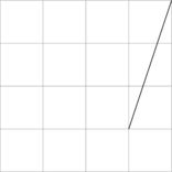
The following minimum syntax just produces a diagonal line. The syntax's are intended as templates around which to construct more substantive code.
| LaTeX code | PDF result |
|---|---|
  \documentclass{standalone}
  \usepackage{tikz}
  \begin{document}
  \begin{tikzpicture}
  \draw (0,0) -- (1,1);
  \end{tikzpicture}
  \end{document}
|
 |
In the above, the tikzpicture environment defined in the tikz package prepares the canvas for graphical instructions. The line starting with the \draw kwyword is an example of a tikz instruction.
I will go into more detail about the \draw keyword later in the tutorial, yet as this routine is used to help outline the concepts of coordinates, I should description is necessary. \draw draws a line between two points (coordinates). The syntax is \draw keyword first (coordinate) two dashes (--) second (coordinate) and the statement is completed by a semi-colon (;).
A more complete minimum example that loads up more tikz extension libraries (those that build on tikz), would be:
| LaTeX code | PDF result |
|---|---|
  \documentclass{standalone}
  \usepackage{tikz}
  \usetikzlibrary{arrows,shadows,positioning,mindmap}
  \usetikzlibrary{decorations, decorations.pathreplacing,decorations.pathmorphing}
  \usetikzlibrary{shapes,shadings,shapes.geometric, shapes.multipart,patterns}
  \usetikzlibrary{backgrounds,calc,fit}
  \begin{document}
  \begin{tikzpicture}
  \draw (0,0) -- (1,1);
  \end{tikzpicture}
  \end{document}
|
 |
The tikzpicture environment
The basic structure of the tikzpicture environment is as follows:
+\n begin{tikzpicture}[]
  (tikz commands);
  \end{tikzpicture}
The options apply to any and all of the elements within the graphic (unless they are specifically overridden by the element). There are approximately 750 options that can be applied to graphical elements (and thus the tikzpicture environment). Some of the most common options that are applied at the environment level so that they affect all elements therein include:
| Option | Description |
|---|---|
| scale=(factor) | Rescaling the graphic by X (e.g. scale=2.5) |
| xscale=(factor), yscale=(factor) | Rescaling x and y separately |
Coordinates
To help demonstrate coordinate concepts, I will make use of an inbuilt grid that can be placed on a graphic. This grid makes it easier to visualize the coordinate system and is therefore a helpful device.
| LaTeX code | PDF result |
|---|---|
Generate a grid from (-2,-2) to (2,2) - (0,0) in the middle
  \begin{tikzpicture}
  \draw [help lines] (-2,-2) grid (2,2);
  \end{tikzpicture}
|
 |
Specifying
Coordinates are specified in brackets
Cartesian: comma separated (x,y)Polar: colon separated (length:angle)
By default, the units are in centimeters for Cartesian (centimeters and degrees for Polar), however, all other valid LaTeX length units can be used.
  (2,4)
  (1pt,5cm)
  (2em,6mm)
| LaTeX code | PDF result |
|---|---|
|
Draw a line starting in the top right corner (2,2) down to the the coordinate (1,-1)
  \begin{tikzpicture}
  \draw [help lines] (-2,-2) grid (2,2);
  \draw (2,2) -- (1,-1cm);
  \end{tikzpicture}
|
 |
A positive x value is to the right, a positive y value is up.
Relative coordinates
Coordinates relative to the previous position can be specified by appending either ++ (incremental) or + (non=incremental) before the brackets.
| Relative coordinates | Description | Examples | |
|---|---|---|---|
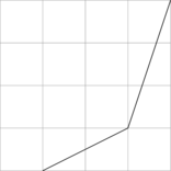
| Incremental (++) | Move from previous point and set the new reference location as the current point |
+\n begin{tikzpicture}
+\n draw [help lines] (-2,-2) grid (2,2);
+\n draw (2,2) -- ++(-1,-3cm) -- ++(-2,-1);
+\n end{tikzpicture}
|
|
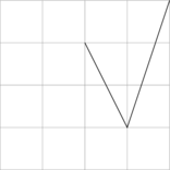
| Non-incremental (+) | Move from previous point but do not set the new reference location as the current point |
+\n begin{tikzpicture}
+\n draw [help lines] (-2,-2) grid (2,2);
+\n draw (2,2) -- +(-1,-3cm) -- +(-2,-1);
+\n end{tikzpicture}
|
|
Storing coordinates
Coordinates can be stored and referenced in other elements.
| LaTeX code | PDF result |
|---|---|
\begin{tikzpicture}
\draw [help lines] (-2,-2) grid (2,2);
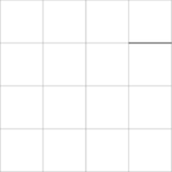
\coordinate (A) at (1,1);
\draw (A) -- ++(1,0);
\end{tikzpicture}
|
 |
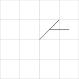
The coordinate specifier can also be used straight after a coordinate is indicated so as to store that coordinate.
| LaTeX code | PDF result |
|---|---|
\begin{tikzpicture}
\draw [help lines] (-2,-2) grid (2,2);
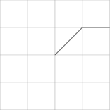
\draw (0,0) -- (1,1) coordinate (A);
\draw (A) -- ++(1,0);
\end{tikzpicture}
|
 |
Modifying coordinates - coordinate calculations
Coordinates can themselves be more complex operations on coordinates.
This is supported by the calc tikz extension package.
The general syntax for coordinate calculations is:
($<factor*><coordinate calculations>$)
The coordinate calculations can then have a series of at least one of the following
separated by + or -:
<factor*><coordinate><modifiers>
The following table outlines the above syntax with each of the major coordinate modification types.
| Coordinate modifier | Description | Examples | |
|---|---|---|---|
| Factors | Optional multipliers |
+\n begin{tikzpicture}
+\n draw [help lines] (-2,-2) grid (2,2);
+\n draw (0,0) -- ($2*(1,1)$);
+\n draw (-1,1) -- (${3*(1-0.9)}*(1,1)$);
+\n end{tikzpicture}
|
 |
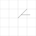
| Addition/subtraction | Set a coordinate to be relative to specified coordinate |
+\n begin{tikzpicture}
+\n draw [help lines] (-2,-2) grid (2,2);
+\n draw (0,0) -- (1,1) coordinate (A);
+\n draw ($(A) +(0,-1)$) -- ++(1,0);
+\n end{tikzpicture}
|
 |
| Fractional Partway | Set a coordinate to be a fraction of the distance partway between two coordinates |
+\n begin{tikzpicture}
+\n draw [help lines] (-2,-2) grid (2,2);
+\n draw (0,0) coordinate (A) -- (1,1)
coordinate (B);
+\n draw ($(A) !0.5! (B)$) -- ++(1,0);
+\n end{tikzpicture}
|
 |
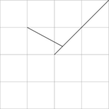
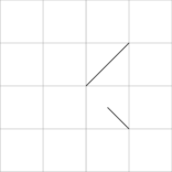
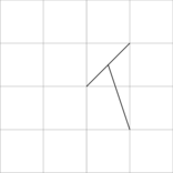
| Use fractional partway to get a length and then specify a relative angle from the first coordinate |
+\n begin{tikzpicture}
+\n draw [help lines] (-2,-2) grid (2,2);
+\n draw (0,0) coordinate (A) -- (1,1)
coordinate (B);
+\n draw ($(A) !0.5!-90: (B)$) -- (1,-1);
+\n end{tikzpicture}
|
 |
|
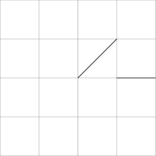
| Distance Partway | Set a coordinate to be a specified distance from the first coordinate along a partway between two coordinates |
+\n begin{tikzpicture}
+\n draw [help lines] (-2,-2) grid (2,2);
+\n draw (0,0) coordinate (A) -- (1,1)
coordinate (B);
+\n draw ($(A) !0.5cm! (B)$) -- ++(1,0);
+\n end{tikzpicture}
|
 |
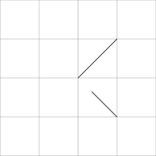
| Use distance partway to get a length and then specify a relative angle from the first coordinate |
+\n begin{tikzpicture}
+\n draw [help lines] (-2,-2) grid (2,2);
+\n draw (0,0) coordinate (A) -- (1,1)
coordinate (B);
+\n draw ($(A) !0.5cm!-90: (B)$) -- (1,-1);
+\n end{tikzpicture}
|
 |
|
| Go to a coordinate along the path between the start and end coordinate that is orthogonal to the projection coordinate |
+\n begin{tikzpicture}
+\n draw [help lines] (-2,-2) grid (2,2);
+\n draw (0,0) coordinate (A) -- (1,1)
coordinate (B);
+\n coordinate (C) at (1,0);
+\n draw ($(A) !(C)! (B)$) -- (1,-1);
+\n end{tikzpicture}
|
 |
Lines and Paths
A path is a series of line segments (straight or curved) between coordinates and is specified by the \path command. By default, a path is invisible.
| Options | Description | Examples | |
|---|---|---|---|
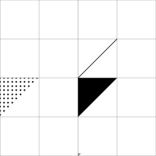
| Path Actions |
draw fill pattern shade \draw is the same as \path [draw] etc |
+\n begin{tikzpicture}
+\n draw [help lines] (-2,-2) grid (2,2);
+\n path [draw] (0,0) -- (1,1);
+\n path [fill] (0,0) -- (1,0) -- (0,-1);
+\n path [pattern] (-2,0) -- (-1,0) -- (-2,-1);
+\n path [shade] (0,-1) -- (1,-1) -- (0,-2);
+\n end{tikzpicture}
|
 |
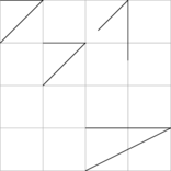
| Geometric Actions |
rotate=<angle> xshift=<length> yshift=<length> scaling=<factor> xscale=<factor> yscale=<factor> |
+\n begin{tikzpicture}
+\n draw [help lines] (-2,-2) grid (2,2);
+\n draw (-2,2) -- (-1,2) -- (-2,1);
+\n draw [rotate around={45:(1,2)}] (0,2) -- (1,2) --
                    (0,1);
+\n draw [xshift=-1cm] (0,1) -- (1,1) -- (0,0);
+\n draw [xscale=2] (0,-1) -- (1,-1) -- (0,-2);
+\n end{tikzpicture}
|
 |
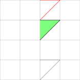
| Color |
color=<color name> draw=<line color> fill=<fill color> opacity=<factor> |
+\n begin{tikzpicture}
+\n draw [help lines] (-2,-2) grid (2,2);
+\n draw [color=red] (0,2) -- (1,2) -- (0,1);
+\n draw [fill=green!50] (0,1) -- (1,1) -- (0,0);
+\n draw [opacity=0.5] (0,-1) -- (1,-1) -- (0,-2);
+\n end{tikzpicture}
Named colors

|
 |
| Line width |
line width=<dimension> ultra thin very thin thin semithick thick very thick ultra thick |
+\n begin{tikzpicture}
+\n draw [help lines] (-2,-2) grid (2,2);
+\n draw [very thick] (0,2) -- (1,2) -- (0,1);
+\n draw [line width=4pt] (0,1) -- (1,1) -- (0,0);
+\n draw [thin] (0,-1) -- (1,-1) -- (0,-2);
+\n end{tikzpicture}
Named colors

|
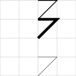 |
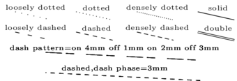
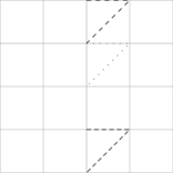
| Line type |
solid dashed dotted dashdotted densely dotted loosely dotted double dash pattern=<pattern> dash phase=<phase> |
+\n begin{tikzpicture}
+\n draw [help lines] (-2,-2) grid (2,2);
+\n draw [dashed] (0,2) -- (1,2) -- (0,1);
+\n draw [loosely dotted] (0,1) -- (1,1) -- (0,0);
+\n draw[densely dashed] (0,-1) -- (1,-1) -- (0,-2);
+\n end{tikzpicture}
Named colors
|
 |
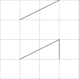
Straight paths/lines
Lines can be drawn by either using the draw path option or the \draw keyword.
| LaTeX code | PDF result |
|---|---|
+\n begin{tikzpicture}
+\n draw [help lines] (-2,-2) grid (2,2);
+\n path [draw] (-1,1) -- (1,2);
+\n draw (-1,-1) -- (1,0) -- (1,-1);
+\n end{tikzpicture}
|
 |
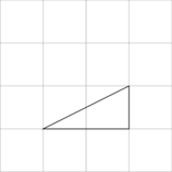
A path can be closed with the --cycle operation
| LaTeX code | PDF result |
|---|---|
+\n begin{tikzpicture}
+\n draw [help lines] (-2,-2) grid (2,2);
+\n draw (-1,-1) -- (1,0) -- (1,-1) --cycle;
+\n end{tikzpicture}
|
 |
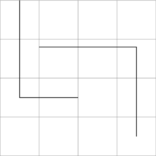
Points can be connected by an 'elbow' including only a horizontal and vertical line rather than a single straight line.
| LaTeX code | PDF result |
|---|---|
+\n begin{tikzpicture}
+\n draw [help lines] (-2,-2) grid (2,2);
+\n draw (-1.5,2) |- (0.0,-0.5);
+\n draw (-1,0.8) -| (1.5,-1.5);
+\n end{tikzpicture}
|
 |
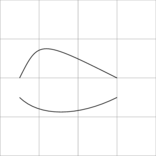
Bezier curved paths/lines
Bazier curves are specified by including .. controls () .. command between points. The coordinates of the controls define the Bezier curve handles.
| LaTeX code | PDF result |
|---|---|
  \begin{tikzpicture}
  \draw [help lines] (-2,-2) grid (2,2);
  \draw (-1.5,0) .. controls (-1,1) .. (1,-0);
  \draw (-1.5,-0.5) .. controls (-1,-1) and (0,-1) .. (1,-0.5);
  \end{tikzpicture}
|
 |
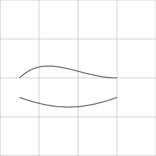
Other curves
It is also possible to create parabola curved paths/lines by a to operation. Exit and entry angles can be respectively defined by the out= and in= options. Alternatively, the bend option can be used to indicate the direction (left or right) and angle of a bend in the path/line. Also consider the following options
- (in,out) looseness
- (in,out) (min,max) distance
- (in,out) control
| LaTeX code | PDF result |
|---|---|
  \begin{tikzpicture}
  \draw [help lines] (-2,-2) grid (2,2);
  \draw (-1.5,0) to [out=45,in=180] (1,-0);
  \draw (-1.5,-0.5) to[bend right=20] (1,-0.5);
  \end{tikzpicture}
|
 |
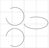
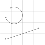
Arc paths/lines
Arcs(of circles or elipses) are achieved via the arc command. An arc is defined by three
parameters separated by colons:
(out angle;in angle;radius length). If only a single radius length
is given, an arc is drawn, if two radius lengths are given, an ellipse is drawn. The sign of the
radius determines the orientation of the arc.
| LaTeX code | PDF result |
|---|---|
+\n begin{tikzpicture}
+\n draw [help lines] (-2,-2) grid (2,2);
+\n draw (-1.5,0.5) arc (10:300:-0.75cm);
+\n draw (-1.5,-1) arc (10:300:-0.75cm and 0.75cm);
+\n draw (0,0) arc (10:300:-1cm and -0.5cm);
+\n end{tikzpicture}
|
 |
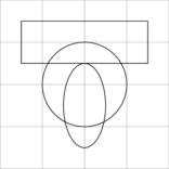
Simple shape paths/lines
There are some pre-defined shapes.geometric
| LaTeX code | PDF result |
|---|---|
+\n begin{tikzpicture}
+\n draw [help lines] (-2,-2) grid (2,2);
+\n draw (-1.5,1.5) rectangle (1.5,0.5);
+\n draw(0,0) circle (1);
+\n draw (0,-0.5) ellipse (0.5 and 1);
+\n end{tikzpicture}
|
 |
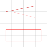
Simple path/line options
| Options | Description | Examples | |
|---|---|---|---|
| color | color of the lines. Can be a mixture of colors. Missing color value treated as 100, missing color treated as white. |
  \begin{tikzpicture}
  \draw [help lines] (-2,-2) grid (2,2);
  \draw [color=red!80!black] (-1.5,1) -- (1,1.5);
  \draw [color=red!40] (-1,1) -- (1,0.5);
  \draw [color=red] (-1.5,-1.5) rectangle (1.5,-0.5);
  \end{tikzpicture}
Named colors
|
 |
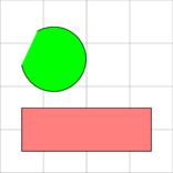
| fill | color of the fill. Can be a mixture of colors. Missing color value treated as 100, missing color treated as white. Named colors same as color |
  \begin{tikzpicture}
  \draw [help lines] (-2,-2) grid (2,2);
  \draw[fill=green] (-1.5,0.5) arc (10:300:-0.75cm);
  \draw[fill=red!50] (-1.5,-1.5) rectangle (1.5,-0.5);
  \end{tikzpicture}
|
 |
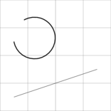
| -> etc | Arrow heads and tails |
+\n begin{tikzpicture}
+\n draw [help lines] (-2,-2) grid (2,2);
+\n draw [<->] (-1.5,0.5) arc (10:300:-0.75cm);
  \draw [|->] (-1.5,-1.5) -- (1.5,-0.5);
  \end{tikzpicture}
Named colors

|
 |
| thin, thick etc | Line thickness |
  \begin{tikzpicture}
  \draw [help lines] (-2,-2) grid (2,2);
  \draw [thin] (-1.5,0.5) arc (10:300:-0.75cm);
  \draw [very thick] (-1.5,-1.5) -- (1.5,-0.5);
  \end{tikzpicture}
Named colors
|
 |
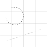
| dashed, dotted etc | Line type |
  \begin{tikzpicture}
  \draw [help lines] (-2,-2) grid (2,2);
  \draw [dashed] (-1.5,0.5) arc (10:300:-0.75cm);
  \draw [dotted] (-1.5,-1.5) -- (1.5,-0.5);
  \end{tikzpicture}
Named colors
|
 |
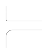
| rounded corners | Rounded corners |
  \begin{tikzpicture}
  \draw [help lines] (-2,-2) grid (2,2);
  \draw[rounded corners] (-1.5,0.5) |- (1.5,-0.25);
  \draw[rounded corners=15pt] (-1.5,-2) |- (1.5,-0.5);
  \end{tikzpicture}
|
 |
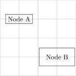
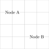
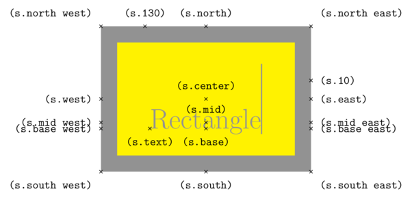
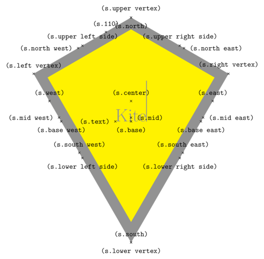
Nodes
A node is a text element placed at a coordinate and optionally may have a simple shape (such as a rectangle or elipse) drawn around it. By default, the shape around a node is stretched such that it just slightly bigger than the contents. A node has a number of anchors as well as a label that can be used to refer to the node (or any of its anchors).
A node has the following syntax:
\node [<options>] (<name>) {<text>};
where the optional name is the node's label and the optional text
is the text element to appear at the node.
| LaTeX code | PDF result |
|---|---|
+\n begin{tikzpicture}
+\n draw [help lines] (-2,-2) grid (2,2);
+\n node at (-1,1) (NodeA) {Node A};
+\n node at (1,-1) (NodeB) {Node B};
+\n end{tikzpicture}
|
 |
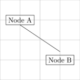
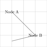
Nodes can also be defined along a path/line by using the node operator in a similar way to the coordinates operator.
| LaTeX code | PDF result |
|---|---|
+\n begin{tikzpicture}
+\n draw [help lines] (-2,-2) grid (2,2);
+\n path [draw] (-1,1) node (NodeA) {Node A} --
(1,-1) node (NodeB) {Node B} -- (-1,-1.5);
+\n end{tikzpicture}
|
 |
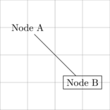
Nodes can be joined via their anchors
| LaTeX code | PDF result |
|---|---|
+\n begin{tikzpicture}
+\n draw [help lines] (-2,-2) grid (2,2);
+\n node at (-1,1) (NodeA) {Node A};
+\n node [draw] at (1,-1) (NodeB) {Node B};
+\n draw (NodeA) -- (NodeB);
+\n end{tikzpicture}
|
 |
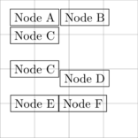
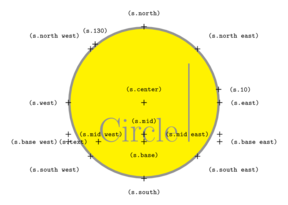
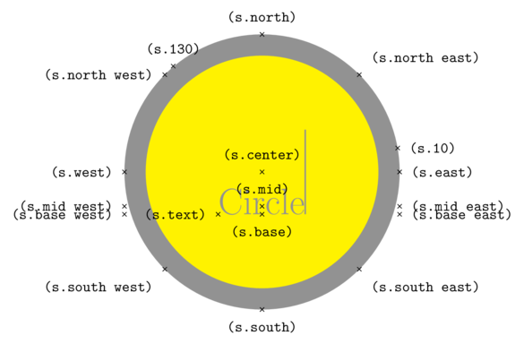
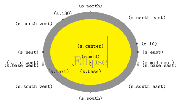
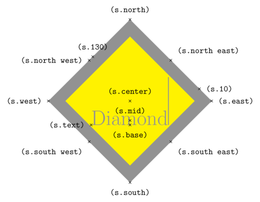
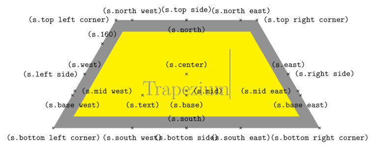
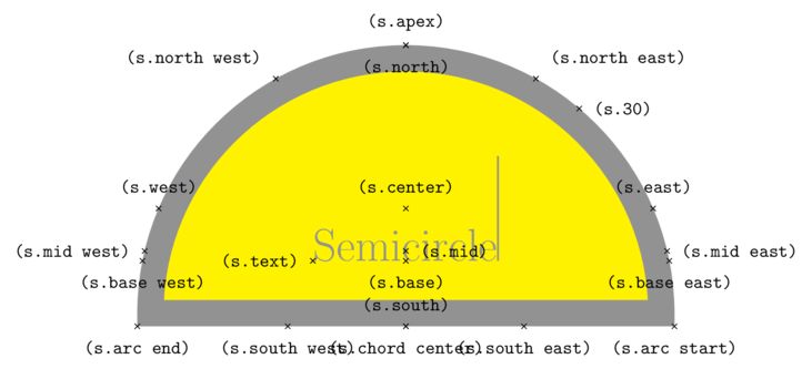
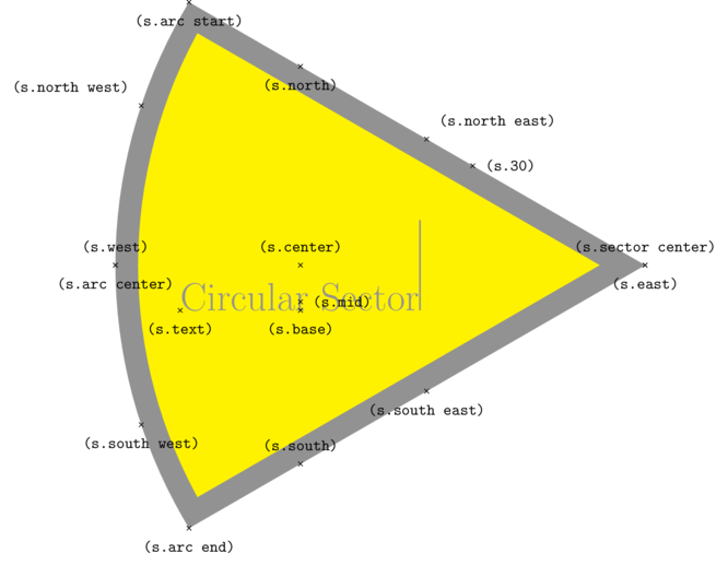
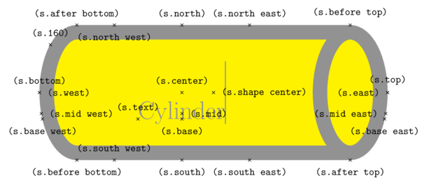
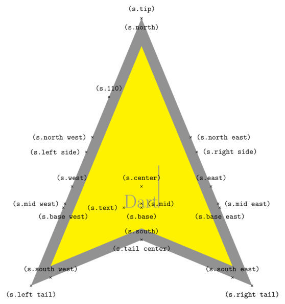
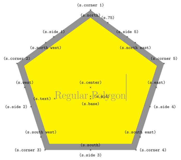
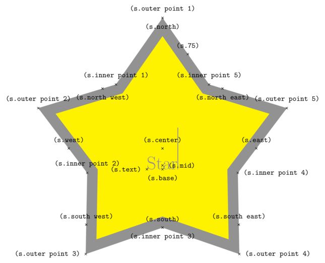
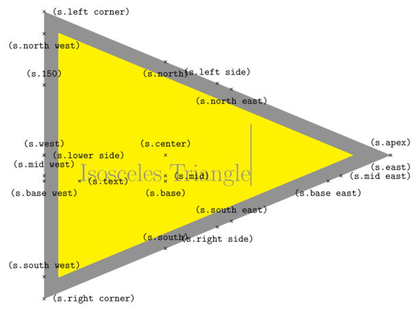
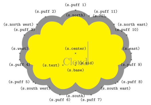
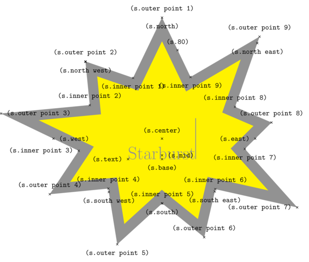
The following shapes are available:
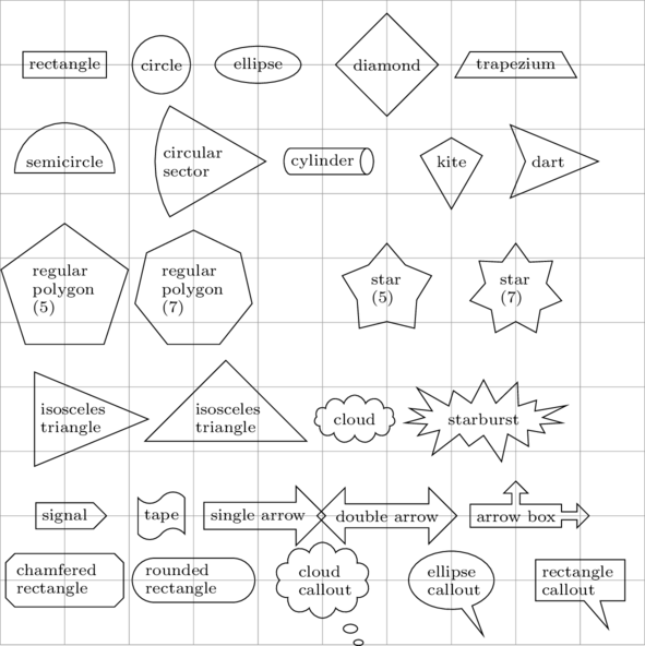
For each of the shapes, there are a number of anchors are available. The following cascading list
features figures modified from the excellent pgf manual that illustrate the anchors associated with each shape.
|
|
|
|
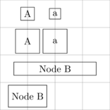
Node options
| Options | Description | ||
|---|---|---|---|
| Inner separation |
Space between text element and node shape boundary inner sep=<dimension>
|
||
| Outer separation |
Space between node shape boundary and anchors outer sep=<dimension>
|
||
| Anchor location |
Anchor location anchor=<direction> or where direction is one of 'north','south','east','west' or a combination <direction>=of <node> where direction is one of 'above','below','left','right' or a combination
|
||
| Minimum size |
Minimum height and/or width minimum size=<dimension>, minimum width=<dimension>, minimum height=<dimension> This provides a way of ensuring that the size of the node is not solely dependent on the size of the node contents.
|
||
| Shape aspect ratio |
The aspect ratio of shapes. This allows a square minimum size=<dimension>, minimum width=<dimension>, minimum height=<dimension> This provides a way of ensuring that the size of the node is not solely dependent on the size of the node contents.
|