Tutorial 2.2 - Importing (reading) and exporting (writing) data
07 Mar 2017
Statistical systems are typically not very well suited to tasks of data entry and management. This is the roll of spreadsheets and databases, of which there are many available. Although the functionality of R continues to expand, it is unlikely that R itself will ever duplicate the extensive spreadsheet and database capabilities of other software. However, there are numerous projects in early stages of development that are being designed to offer an interface to R from within major spreadsheet packages.
R development has roots in the Unix/Linux programming philosophy that dictates that tools should be dedicated to performing specific tasks that they perform very well and rely on other tools to perform other tasks. Consequently, the emphasis of R is, and will continue to be, purely an environment for statistical and graphical procedures. It is expected that other software will be used to generate and maintain data sets.
Unfortunately, data importation into R can be a painful exercise that overshadows the benefits of using R for new users. In part, this is because there are a large number of competing methods that can be used to import data and from a wide variety of sources. Moreover, many of the popular spreadsheets use their own proprietary file formats that are particularly complex to accommodate fully.
This section does not intend to cover all the methods. Rather, it will highlight the simplest and most robust methods of importing data from the most popular sources. Unless file path names are specified, all data reading functions will search for files in the current working directory.
Importing from text file
The easiest form of importation is from a pure text file. Since most software that accepts file input can read plain text files, text files can be created in all spreadsheet, database and statistical software packages and are also the default outputs of most data collection devices.
In a text file, data are separated (or delimited) by a specific character, which in turn defines what sort of text file it is. The text file should broadly represent the format of the data frame.
- variables should be in columns and sampling units in rows.
- the first row should contain the variable names and if there are row names, these should be in the first column
The following examples illustrate the format of the abbreviated Mac Nally (1996) data set created as both comma delimited (left) and tab delimited (right) files as well as the corresponding read.table() commands used to import the files.
Obtain the necessary files (macnally.csv, macnally.txt) by either:
- clicking on this link and this link OR
- from inside R, run execute the following (will download the files to your home directory):
download.file('http://www.flutterbys.com.au/stats/downloads/data/macnally.csv', '~/macnally.csv')
Note, the following examples assume that the current working directory contains the data sets (macnally.csv and macnally.txt). If the current working directory (can be checked with the getwd() function) does not contain these files, then either:
- include the full path name (or path relative to the current working directory) as the filename argument
- change the current working directory of your session prior to continuing (use the setwd() function
- copy and paste the files into the current working directory
| Comma delimited text file *.csv | Tab delimited text file *.txt | |||||||||||||||||||||
|---|---|---|---|---|---|---|---|---|---|---|---|---|---|---|---|---|---|---|---|---|---|---|
,HABITAT,GST,EYR Reedy Lake,Mixed,3.4,0.0 Pearcedale,Gipps.Manna,3.4,9.2 Warneet,Gipps.Manna,8.4,3.8 Cranbourne,Gipps.Manna,3.0,5.0 .... |
|
|||||||||||||||||||||
MACNALLY <- read.table('macnally.csv', header=T, row.names=1, sep=',', strip.white=TRUE) |
MACNALLY <- read.table('macnally.txt', header=T, row.names=1, sep='\t', strip.white=TRUE) |
The read.table() function accommodates the importation of a broad range of text file that basically represent a table or data. There are also more specific versions (read.csv() and read.delim()) that use different defaults as appropriate for reading in comma and tab delimited files respectively. Fixed with delimited text files can be read in with the read.fwf() function.
The strip.white=TRUE argument indicates that leading and trailing spaces should be removed from all the data. This is important as often spreadsheets (I'm looking at you Excel), add spaces before or after words (in particular). These are invisible, yet can cause huge headaches when running analyses or graphing..
Full path
In the above code snippets, the files were assumed to be in the current working directory. Lets instead read in the macnally.csv file from a different location by including the full path.
MACNALLY <- read.table('/home/murray/Work/stats/downloads/data/macnally.csv', header=T, row.names=1,
  sep=',', strip.white=TRUE)
Relative path
# go into a sub-directory of the current directory
MACNALLY <- read.table('data/macnally.csv', header=T, row.names=1, sep=',', strip.white=TRUE)
# go out of the current directory and into a sibling directory
MACNALLY <- read.table('../data/macnally.csv', header=T, row.names=1, sep=',', strip.white=TRUE)
URL
MACNALLY <- read.table(
  url('http://www.flutterbys.com.au/stats/downloads/data/macnally.csv'),
  header=T, row.names=1, sep=',', strip.white=TRUE)
For csv (comma separated files), there is also a more specific function - read.csv().
MACNALLY <- read.csv('macnally.csv',row.names=1, strip.white=TRUE)
Importing from the clipboard
The read.table() function can also be used to import data (into a data frame) that has been placed on the clipboardb by other software, thereby providing a very quick and convenient way of obtaining data from spreadsheets. Simply replace the filename argument with the word 'clipboard' and indicate a tab field separator (\t). For example, to import data placed on the clipboard from Microsoft Excel, select the relevant cells, click copy and then in R, use the following syntax;
MACNALLY2 <- read.table('clipboard', header=TRUE, row.names=1, sep="\t")
Importing from other software
As previously stated, virtually all software packages are able to export data in text file format and usually with a choice of delimiters. However, the foreign package offers more direct import of native file formats from a range of other popular statistical packages. To illustrate the use of the various relevant functions within the foreign package, importation of a subset of the Mac Nally (1996) data set from the various formats will be illustrated.
Systat
library(foreign)
MACNALLY2 <- read.systat('macnally.syd', to.data.frame=TRUE)
Although note that this cannot be used to import files produced with the MacOSX version of SYSTAT due to inpompatibile file formats.
Spss
library(foreign)
MACNALLY2 <- read.spss('macnally.sav', to.data.frame=TRUE)
Minitab
library(foreign)
MACNALLY2 <- as.data.frame(read.mtp('macnally.mtp'))
SAS
library(foreign)
MACNALLY2 <- read.xport('macnally')
Note, the file nust be in the SAS XPORT format. If there is only a single dataset in the XPORT format library, then the read.xport() function will return a data frame, otherwise it will return a list of data frames.
Excel
Excel is more than just a spreadsheet – it contains macros, formulae, multiple worksheets and formatting. There are numerous ways to import xlsx files into R, yet depending on the complexity of the original files, the translations can be incomplete and inconsistent.
The easiest and safest ways to import data from Excel is either to save the worksheet as a text file (comma or tab delimited) and import the data as a text file (see above), or to copy the data to the clipboard in Excel and import the clipboard data into R.
Exporting to a text file
Although plain text files are not the most compact storage formats, they do offer two very important characteristics. Firstly, they can be read by a wide variety of other applications, ensuring that the ability to retrieve the data will continue indefinitely. Secondly, as they are neither compressed nor encoded, a corruption to one section of the file does not necessarily reduce the ability to correctly read other parts of the file. Hence, this is also an important consideration for the storage of datasets.
The write.table() function is used to save data frames. Although there are a large number of optional arguments available for controlling the exact format of the output file, typically only a few are required. The following example illustrates the exportation of the Mac Nally (1996) data set as a comma delimited text file.
write.table(MACNALLY, 'macnally.csv', quote=F, row.names=T, sep=',')
The first and second arguments specify respectively the name of the data frame and filename (and path if necessary) to be exported. The quote=F argument indicates that words and factor entries should not be exported with surrounding double quotation marks. Note, if you have a column (field) in your data that is a string with commas (such as site descriptions etc), then you should use quote=TRUE.
The row.names=T argument indicates that the row names in the data frame are also to be exported (they will be the first column in the file). If there are no defined row names in the data frame, alter the argument to row.names=F. Finally, specify the field separator for the file (comma specified in above example).
As with reading text files, for csv files, there is a more specific version - write.csv()
.write.csv(MACNALLY, 'macnally.csv', quote=F, row.names=T)
Saving and loading R objects
Any object in R (including data frames) can also be saved into a native R workspace image file (*.RData) either individually, or as a collection of objects using the save() function.
Whilst this native R storage format is not recommended for long-term data storage and archival (as it is a binary format and thus less likely to be universally and indefinitely readable), saving and loading of R objects does provide very useful temporary storage of large R objects between sessions.
In particular, if one or more objects require processing or manipulations that take some time to regenerate, saving and loading of R objects can permit the analyst to skip straight to a specific section of a script and continue development or analysis. Moreover, this is very useful for tweaking and regenerating summary figures - rather than have to go through an entire sequence of data reading, processing and analysis, strategic use of saving/loading of R objects can allow the researcher to commence directly at the point at which modification is required.
For example:
#save just the MACNALLY data frame
save(MACNALLY, file='macnally.RData')
#calculate the mean GST
meanGST <- mean(MACNALLY$GST)
#display the mean GST
meanGST
#save the MACNALLY data frame as well as the mean GST object
save(MACNALLY, meanGST, file='macnallystats.RData')
The saved object(s) can be loaded during subsequent sessions by providing the name of the saved workspace image file as an argument to the load() function. For example;
load('macnallystats.RData')
Similarly, a straight un-encoded text version of an object (including a dataframe) can be saved or added to a text file using the dump() function.
dump('MACNALLY',file='macnally')
If the file character string is left empty, the text representation of the object will be written to the console. This output can then be viewed or copied and pasted into a script file, thereby providing a convenient way to bundle together data sets along with graphical and analysis commands that act on the data sets.
dump('MACNALLY',file='')
Thereafter, the dataset is automatically included when the script is sourced and cannot accidentally become separated from the script.
Worked examples
Basic statistics references
- Logan (2010) - Chpt 1, 2 & 6
- Quinn & Keough (2002) - Chpt 1, 2, 3 & 4
Data sets - Data frames(R)
Rarely is only a single biological variable collected. Data are usually collected in sets of variables reflecting tests of relationships, differences between groups, multiple characterizations etc. Consequently, data sets are best organized into collections of variables (vectors). Such collections are called data frames in R.
Data frames are generated by combining multiple vectors together whereby each vector becomes a separate column in the data frame. In for a data frame to represent the data properly, the sequence in which observations appear in the vectors (variables) must be the same for each vector and each vector should have the same number of observations. For example, the first observations from each of the vectors to be included in the data frame must represent observations collected from the same sampling unit.
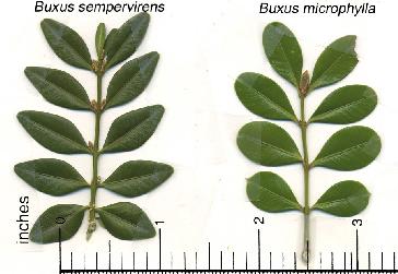
To demonstrate the use of dataframes in R, we will use fictitious data representing the areas of leaves of two species of Japanese Boxwood
| Format of the fictitious data set | ||||||||||||||||||||||||||||
|---|---|---|---|---|---|---|---|---|---|---|---|---|---|---|---|---|---|---|---|---|---|---|---|---|---|---|---|---|
|
 |
|||||||||||||||||||||||||||
- Lets create the data set in a series of steps. Use the textbox provided in part g below to record the R syntax used in each step
- First create the categorical (factor) variable containing the listing of B.semp three times and B.micro three times
- Now create the dependent variable (numeric vector) containing the leaf areas
- Combine the two variables (vectors) into a single data set (data frame) called LEAVES
- Print (to the screen) the contents of this new data set called LEAVES
- You will have noticed that the names of the rows are listed as 1 to 6 (this is the default). In the table above, we can see that there is a variable called PLANT that listed unique plant identification labels. These labels are of no use for any statistics, however, they are useful for identifying particular observations. Consequently it would be good to incorporate these labels as row names in the data set. Create a variable called PLANT that contains a listing of the plant identifications
- Use this plant identification label variable to define the row names in the data frame called LEAVES
- In the textbox provided below, list each of the lines of R syntax required to generate the data set
Show codeSPECIES <- gl(2,3,6,lab=c('B.semp', 'B.micro')) AREA <- c(25,22,29,15,17,20) LEAVES <- data.frame(SPECIES,AREA) LEAVES
  SPECIES AREA
1  B.semp   25
2  B.semp   22
3  B.semp   29
4 B.micro   15
5 B.micro   17
6 B.micro   20
PLANT <- c('P1','P2','P3','P4','P5','P6')
#OR
PLANT <- paste('P',1:6,sep="")
row.names(LEAVES) <- PLANT
PLANT
[1] "P1" "P2" "P3" "P4" "P5" "P6"
The above syntax forms a list of instructions that R can perform. Such lists are called scripts. Scripts offer the following;
- Enable a sequence of tasks such as data entry, analysis and graphical preparation to be repeated quickly and precisely
- Ensure that the sequence of tasks used to complete an analysis are permanently documented
- Simplify performing many similar analyses
- Simplify sharing of data, analyses and techniques
- To see how to use a script,
- close down R
- restart R
- Change the working directory (path) to the location where you saved the script file in Q4.2 above
- Source the script file
- There are now at least four objects in the
R workspace.
These should be LEAVES (the data frame - data set), PLANTS (the list of plant ID's), SPECIES (the character vector of plant species) and AREA (the numeric vector of leaf areas).
- Print (list on screen) the contents of the AREA vector. Note, that this is listing the contents of the AREA vector, this is not the same as asking it to list the contents of the AREA vector within the LEAVES data frame. For example, multiply all of the numbers in the AREA vector by 2. Now print the contents of the AREA vector then the LEAVES data frame. Notice that only the values in the AREA vector have changed - the values within the AREA vector of the LEAVES data frame were not effected.
- To avoid confusion and clutter, it is therefore always best to remove single vectors once a data frame has been created. Remove the PLANTS, SPECIES and AREA vectors.
- Notice what happens when you now try to access the AREA vector.
- To access a variable from within a data frame, we use the $ sign. Print the contents of the LEAVES AREA vector
- Since data are stored in vectors, it is possible to access single entries or specific groups of entries. A specific entry is accessed via its
index.
To investigate the range of options, complete the following table.
Access Syntax print the LEAVES data set hint print first leaf area in the LEAVES data set hint print the first 3 leaf areas in the LEAVES data set hint print a list of leaf areas that are greater than 20 hint print a list of leaf areas for the B.microphylum species hint print the section of the data set that contains the B.microphylum species hint alter the second leaf area from 22 to 23 hint Show codeLEAVESSPECIES AREA P1 B.semp 25 P2 B.semp 22 P3 B.semp 29 P4 B.micro 15 P5 B.micro 17 P6 B.micro 20
LEAVES$AREA[1]
[1] 25
LEAVES$AREA[1:3]
[1] 25 22 29
LEAVES$AREA[LEAVES$AREA>20]
[1] 25 22 29
LEAVES$AREA[LEAVES$SPECIES=='B.micro']
[1] 15 17 20
LEAVES[LEAVES$SPECIES=='B.micro',]
   SPECIES AREA
P4 B.micro   15
P5 B.micro   17
P6 B.micro   20
LEAVES$AREA[2] <- 23
- Although it is possible to some data editing this way, for more major editing procedures it is better to either return to Excel or use the
'fix()' function.
Use the 'fix()' function to make a number of changes to the data frame (data set) including adding another column of data (that might represent another variable).
- Sometimes it is necessary to
transform
a variable from one scale to another. While it is possible to modify an existing variable (vector), it is safer to create a new variable that contains the altered values.
Examine the use of R for common transformations.
Transform the leaf areas to log (base 10).
Show codeLEAVES$logAREA <- log10(LEAVES$AREA)
Importing data and data files
Although it is possible to generate a data set from scratch using the procedures demonstrated in the above demonstration module, often data sets are better managed with spreadsheet software. R is not designed to be a spreadsheet, and thus, it is necessary to import data into R. We will use the following small data set (in which the feeding metabolic rate of stick insects fed two different diets was recorded)to demonstrate how a data set is imported into R.
| Format of the fictitious data set | ||||||||||||||||||||||||||||
|---|---|---|---|---|---|---|---|---|---|---|---|---|---|---|---|---|---|---|---|---|---|---|---|---|---|---|---|---|
|
 |
|||||||||||||||||||||||||||
- Importing data into R from Excel is a multistage stage process.
- Enter the above data set into Excel and save the sheet as a comma delimited text file (CSV)
. Ensure that
e column titles (variable names) are in the first row and that you take note where the file is saved. To see the format of this file, open it in Notepad (the windows accessory program). Notice that it is just a straight text file, there is no encryption or encoding. - Ensure that the current working directory is set to the location of this file
- Read (import) the data set into a data table . Since data exploration and analysis cannot begin until the data is imported into R, the syntax of this step would usually be on the first line in a new script file that is stored with the comma delimited text file version of the data set.
- To ensure that the data have been successfully imported, print the data frame
Show codesetwd("../downloads/data")
Error in setwd("../downloads/data"): cannot change working directoryphasmid <- read.table('phasmid.csv', header=T, sep=',', row.names=1)
Error in file(file, "rt"): cannot open the connection
- Enter the above data set into Excel and save the sheet as a comma delimited text file (CSV)
. Ensure that
- As well as importing files, it is often necessary to save a data set (data frame) - particularly if it has been modified and you wish to retain the changes. To demonstrate how to export a data set, we need a data frame (data set) to export. If the LEAVES data frame (from above) is no longer present, regenerate the LEAVES data set from above
using the script file
that was generated in Q1-2. To export an R data frame to a text file, you need to
write the data frame to a file
- Examine the contents of this comma delimited text file using Notepad
- Alternatively, it is also possible to copy and paste data from Excel into R (via the clipboard).
Although this method is quicker, there is no record in a R script file as to which Excel file the data originally came from.
Furthermore, changes to the Excel data sheet will not be accounted for.
Read the data in from the clipboard.
Show code
phasmid <- read.table('clipboard', header=T, sep='\t', row.names=1)
- Since there is no link between the data and the script when data are imported via the clipboard, it is recommended
that the data be stored as a structure within your R script above any commands that use these data.
Place a copy of the data within the R script file that you generated earlier..
Show code
dump('phasmid',"")
phasmid <-
structure(list(DIET = structure(c(2L, 2L, 2L, 1L, 1L, 1L), .Label = c("soft",
"tough"), class = "factor"), MET.RATE = c(1.25, 1.22, 1.29, 1.51,
1.55, 1.48)), .Names = c("DIET", "MET.RATE"), class = "data.frame", row.names = c("P1",
"P2", "P3", "P4", "P5", "P6"))
Show codewrite.table(LEAVES, 'leaves.csv', quote=F, sep=',')