Tutorial 2.4 - Data manipulation
27 Mar 2017
I apologize in advance, this tutorial requires quite a bit of explaining and context before it can get into the code.... Good data manipulation is an art form that requires the use of many specific tools (functions) and expert data manipulation comes from the integration of these tools together. Therefore it is necessary to have an overview of the tool set before investigating any single tool.
Manipulating data sets
Rarely are data transcribed and organized into such simple and ready-to-go data sets. More typically, data are spread throughout multiple sources and in a variety of formats (particularly if compiled by multiple workers or instruments). Consequently, prior to any formal statistical analyses , it is necessary to compile very focused, tidy data sets.
Wickham (2014) suggests that there are many ways to organise data, yet tidy data (data that
are structured in such a consistent way as to facilitate analyses) must adhere to a fairly strict set of structural rules. Specifically,
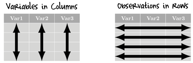
in tidy data:
- variables are in columns
- observations are in rows - that is, for univariate data, there should be a separate row for each response observation.
To achieve tidy data, common data preparations include:
- Reshaping and rearranging data
- Merging multiple data sources
- Aggregating data to appropriate spatial/temporal scales
- Transforming data and deriving new variables
- Sorting and reordering data
- Relabelling data
Practical data manipulation will be demonstrated via a series of very small artificial datasets. These datasets are presented in tables with black font and lines and the R code required to generate those data will be presented in static code boxes either underneath or adjacent the table. A very basic description of the table and the name of the data frame are displayed above the table. The entire collection of datasets used in this workshop can be obtained by issuing the following command:
- (if online)
source(url( "http://www.flutterbys.com.au/stats/downloads/data/manipulationDatasets.R"))
#OR
load("http://www.flutterbys.com.au/stats/downloads/data/manipulationDatasets.RData")
- (if offline and are running this from a local version having first downloaded either file)
source(file="manipulationDatasets.R")
#OR
load("manipulationDatasets.RData")
The great folks over at Rstudio have produced an excellent set of cheatsheets on a range of topics. For this tutorial, the Data Import Cheat Sheet (mainly page 2) and Data Transformation Cheat Sheet are useful summaries.
tidyverse a data manipulation ecosystem within R
There are numerous packages and base R routines devoted to data manipulation. Notable packages include data.tables, plyr and doBy. Indeed, earlier versions of this tutorial featured examples of each of these packages. However, an entire family of packages from Hadley Wickem's group now stands out as a comprehensive, intuitive suite of tools for data manipulation and visualisation.
Importantly, all of these packages are designed to integrate together and complement one another with a consistent interface. Individually, the important relevant packages for this tutorial include:
- dplyr, for data manipulation
- tidyr, for data tidying
- forcats, for factors
To simplify installing an entire data ecosystem, the tidyverse package is available. Installing this package (via install.packages('tidyverse')) will install the following packages:
|
|
Loading the tidyverse() package will automatically load the following packages:
- dplyr, for data manipulation
- tidyr, for data tidying
- ggplot2, for visualising data
- tibble, for a new data.frame-like structure
- readr, for importing data
- purr, for functional programming
library(tidyverse)
library(forcats)
Finally, for much of the rest of the tutorial, I will demonstrate multiple ways to perform the tasks. Whilst the tidyverse ecosystem of packages all integrate well with one another, they do conflict with other packages. Consequently, for the alternate routines I demonstrate, namespaces will be used rather than loading of the associated packages.
The grammar of data manipulation
Hadley and his collaborators argue that there is a grammar of data manipulation and that manipulations comprises the following core verbs:
|
|
Piping
Typically, data manipulation/preparations comprise multiple steps and stages in which a series of alterations, additions etc are performed sequentially such that the data are progressively molded into a form appropriate for analysis etc. Traditionally, this would have involved a separate expression for each step often resulting in the generation of numerous intermediate data sets.
Furthermore, in an attempt to reduce the number of intermediate steps, functions are often nested within other functions such that alterations are made inline within another function. Collectively, these practices can yield code that is very difficult to read and interpret.
A a motivating (if not a bit extreme) example, lets say we wanted to calculate the logSumExp function: $$ log(\sum^{n}_{i=1} e^{x_i}) $$
## Generate some data
set.seed(123)
x = rgamma(10,5,1)
## Calculate the logSumExp
log(sum(exp(x)))
[1] 9.316408
## OR
x1=exp(x)
x2=sum(x1)
log(x2)
[1] 9.316408
A long honoured unix coding principle is that each application should focus on performing one action and performing that function well. In order to perform a sequence of of actions therefore involves piping (via the unix pipe character '|') the output of one application to the input of another application and so on in a chain. The grammar of data wrangling also adopts this principle (each tool specializing on one action and tools should be piped together to achieve a sequence of actions).
The piping (glue) operator in tidyverse is %>%. An object on the left hand side of the %>% operator is passed as the first argument of the function on the right hand side.
x %>% exp %>% sum %>% log
[1] 9.316408
To reiterate, the following two are equivalent:
exp(x)
 [1]   29.653639 1601.918872    5.101634  118.918637 7140.686681  252.361318    9.175114    4.863565 1756.825350
[10]  199.466617
x %>% exp
 [1]   29.653639 1601.918872    5.101634  118.918637 7140.686681  252.361318    9.175114    4.863565 1756.825350
[10]  199.466617
log(x, base=10)
[1] 0.5301465 0.8679950 0.2120706 0.6792861 0.9480981 0.7427928 0.3456667 0.1991438 0.8733941 0.7239190
x %>% log(base=10)
[1] 0.5301465 0.8679950 0.2120706 0.6792861 0.9480981 0.7427928 0.3456667 0.1991438 0.8733941 0.7239190
Most of the following examples will demonstrate isolated data manipulation actions (such as filtering, summarizing or joining) as this focuses on the specific uses of these functions without the distractions and complications of other actions. For isolated uses, piping has little (if any) advantages. Nevertheless, in recognition that data manipulations rarely comprise a single action (rather they are a series of linked actions), for all remaining examples demonstrated in the tidyverse (dplyr/tidyr) context, piping will be used.
Reshaping dataframes
Wide to long (gather)
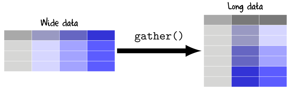
Whilst wide data formats are often more compact and typically easier to manage for data entry (particularly in the field), the data are not in the appropriate format for most analyses (traditional repeated measures and multivariate analyses are two exceptions). Most analyses require that each replicate is in its own row and thus it is necessary to be rearrange or reshape (melt or gather) the data from this wide format to the long (molten) format.
Whilst there are numerous routines in R for reshaping data, we will only explore those that are formally part of the tidyverse ecosystem.
The gather() function (dplyr package) is very useful for converting wide (repeated measures-like) into long format. The important parameters to specify are;
- key, a name for the new categorical variable that represents the levels that correspond to the variables being gathered (shown in purple in the Wide data above)
- value a name for the numeric variable to contain the observations
data.w
|
View code
set.seed(1) data.w <- expand.grid(Plot=paste("P",1:4,sep="")) data.w$Between <- gl(2,2,4,lab=paste("A",1:2,sep="")) data.w <- with(data.w, data.frame(Between,Plot, matrix(rpois(12,10),ncol=3, dimnames=list(paste("R",1:4,sep=""), paste("Time",0:2,sep=":"))))) |
|
Via gather (package:tidyr)
data.w %>% gather(key=Time,value=Count,Time.0,Time.1,Time.2)
#OR
data.w %>% gather(key=Time,value=Count,-Between,-Plot)
Between Plot Time Count 1 A1 P1 Time.0 8 2 A1 P2 Time.0 10 3 A2 P3 Time.0 7 4 A2 P4 Time.0 11 5 A1 P1 Time.1 14 6 A1 P2 Time.1 12 7 A2 P3 Time.1 11 8 A2 P4 Time.1 9 9 A1 P1 Time.2 14 10 A1 P2 Time.2 11 11 A2 P3 Time.2 8 12 A2 P4 Time.2 2 |
When specifying which columns to gather, there are also a number of "Helper" functions that provide convenient ways to select columns:
- contains(""), columns whose name match the character string (not case sensitive by default)
- starts_with(""), columns whose names begin with the character string (not case sensitive by default)
- ends_with(""), columns whose names end with the character string (not case sensitive by default)
- one_of(c("","")), columns whose names are amongst the character strings
- matches(""), columns whose names are matched by the character string of a regular expression (not case sensitive by default)
- everything(), all columns. This is useful in combination with other specifiers
- num_range("",), select all columns whose names start with the first argument (a character string) followed by a number in the integer sequence provided as the second argument
|
Via gather (package:tidyr)
data.w %>% gather(key=Time,value=Count, contains('Time'))
#OR
data.w %>% gather(key=Time,value=Count, num_range('Time.',0:2))
#OR
data.w %>% gather(key=Time,value=Count, matches('Time.[0-2]'))
Between Plot Time Count 1 A1 P1 Time.0 8 2 A1 P2 Time.0 10 3 A2 P3 Time.0 7 4 A2 P4 Time.0 11 5 A1 P1 Time.1 14 6 A1 P2 Time.1 12 7 A2 P3 Time.1 11 8 A2 P4 Time.1 9 9 A1 P1 Time.2 14 10 A1 P2 Time.2 11 11 A2 P3 Time.2 8 12 A2 P4 Time.2 2 |
Long to wide (cast)
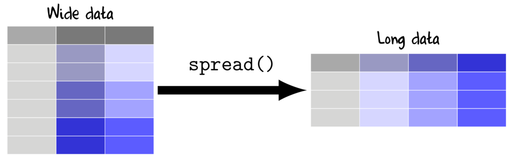
The spread() function (tidyr package) is very useful for converting long datasets into wide (repeated measures-like). The heart of the function definition is specifying a formula LHS ~ RHS where;
- key the existing categorical variable that will define the new variable names
- value the existing numeric variable that will be reshaped into wide format
data
|
View code
data.l = data %>% select(-Resp2) |
| Widen (spread) Resp1 for repeated measures (Within) |
|---|
|
Via spread (package:tidyr)
data.l %>% spread(Within,Resp1) Between Plot Subplot B1 B2 1 A1 P1 S1 8 10 2 A1 P1 S2 7 11 3 A1 P4 S7 8 10 4 A1 P4 S8 7 12 5 A2 P2 S3 14 12 6 A2 P2 S4 11 9 7 A2 P5 S9 11 12 8 A2 P5 S10 12 10 9 A3 P3 S5 14 11 10 A3 P3 S6 8 2 11 A3 P6 S11 3 11 12 A3 P6 S12 13 7 |
If the data are not already fully gathered, then it is necessary to gather before spreading. For example, if we return to the data that contain both Resp1 and Resp2...
data
|
View code
set.seed(1) data <- expand.grid(Within=paste("B",1:2,sep=""), Subplot=paste("S",1:2,sep=""), Plot=paste("P",1:6,sep="")) data$Subplot <- gl(12,2,24,lab=paste("S",1:12,sep="")) data$Between <- gl(3,4,24,lab=paste("A",1:3,sep="")) data$Resp1 <- rpois(24,10) data$Resp2 <- rpois(24,20) data <- with(data,data.frame(Resp1,Resp2,Between,Plot,Subplot,Within)) |
| Widen (spread) both Resp1 and Resp2 for repeated measures |
|---|
Note, the above data are not untidy..
Combining columns (unite)
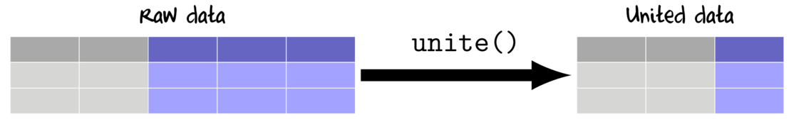
If data are recorded with excessive fidelity, it may be useful to combine multiple fields into a single field. For example, if the date was recorded across three fields (year, month and day, we may like to combine these to form a single date field.
data.d
|
View code
set.seed(1) data.d = data.frame(Date=sample(seq(as.Date('2008-01-01'), as.Date('2009-12-31'), by='day'), size=10), Resp1=rnbinom(10,5,mu=30) * as.numeric(replicate(5, rbinom(2,1,0.8)))) %>% separate(Date,into=c('year','month','day')) |
| Unite year, month and day into a single 'Date' field. |
|---|
|
Via unite (package:tidyr)
data.d %>% unite(year,month,day,col='Date',sep='-') Date Resp1 1 2008-07-13 16 2 2008-09-28 25 3 2009-02-21 52 4 2009-10-23 18 5 2008-05-26 0 6 2009-10-14 45 7 2009-11-15 40 8 2009-04-23 38 9 2009-03-30 9 10 2008-02-14 22 |
In the last spread example, we widened Resp1 and Resp2 for each level of Within. However, we may wish to present this table in a more compact form in which the data are further spread into each combination of Resp and Within. Note, doing so would even more untidy data.
| Unite year, month and day into a single 'Date' field. |
|---|
|
||||||||||||||||||||||||||||||||||||||||||||||||||||||||||||||||||||||||||||||||||||||||||||||||||||||||
|
Via unite (package:tidyr)
data %>% gather(Resp,Count, contains('Resp')) %>% unite(RW, Resp, Within) %>% spread(RW,Count) Between Plot Subplot Resp1_B1 Resp1_B2 Resp2_B1 Resp2_B2 1 A1 P1 S1 8 10 17 18 2 A1 P1 S2 7 11 17 21 3 A1 P4 S7 8 10 17 22 4 A1 P4 S8 7 12 16 13 5 A2 P2 S3 14 12 19 13 6 A2 P2 S4 11 9 24 18 7 A2 P5 S9 11 12 23 19 8 A2 P5 S10 12 10 23 21 9 A3 P3 S5 14 11 25 18 10 A3 P3 S6 8 2 27 22 11 A3 P6 S11 3 11 17 16 12 A3 P6 S12 13 7 26 28 |
Splitting columns appart (separate)
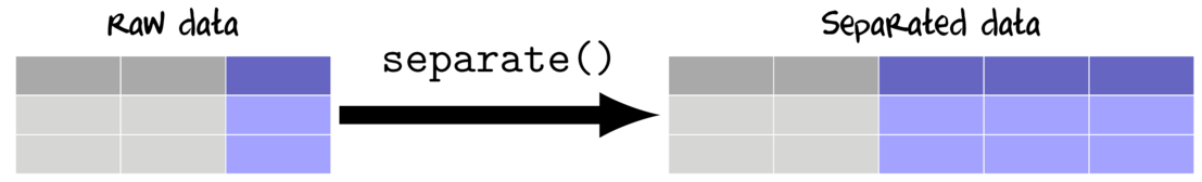
Separating variables is the opposite of uniting them. A field is separated by either indicating a character(s) to use as a separator, or else providing a fixed width format.
data.c
|
View code
set.seed(1) data.c <- data.frame(Year=paste0(sample(c('M','F'),10,replace=TRUE),rpois(10,30)), Resp1=rnbinom(10,5,mu=30) * as.numeric(replicate(5,rbinom(2,1,0.8)))) |
| Separate year, month and day into a single 'Date' field. |
|---|
|
Via separate (package:tidyr)
data.c %>% separate(Year,into=c('Gender','Age'),sep=1) Gender Age Resp1 1 M 25 45 2 M 28 40 3 F 29 38 4 F 43 9 5 M 34 22 6 F 25 20 7 F 26 22 8 F 28 32 9 F 27 38 10 M 29 47 |
Summary and Vectorized functions

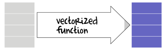
Many data manipulation actions involve the use of specific auxiliary functions to act on specific parts of the data set. For example if we wish to summarize a data set, we might apply a mean() function to the numeric vectors (variables) and levels() or unique function to character or factor vectors. On the other hand, if we wish to generate log-transformed versions of the numeric vectors, the we would apply the log() function to each of those numeric vectors. Furthermore, we might use other auxiliary functions that return vectors of either booleans (TRUE or FALSE) or integers that can represent row or column indices to determine which observations to perform actions on.
Broadly speaking, summary functions take a vector and return a single value. Familiar examples of summary functions are mean(), var(), min() etc. By contrast, vectorized functions take a vector and return a vector of the same length as the original input vector. rank(), cumsum() and log() are all examples of window functions.
The dplyr package introduces a number of additional summary and vectorized functions that are deemed useful augmentations of the standard set of functions available in base R. The following tables describes the most useful functions (from base and dplyr) along with which manipulation functions they can be applied. Those functions defined in dplyr include the dplyr namespace.
To demonstrate summary and vector functions, the following vectors will be used.
## Generate some data
set.seed(123)
(x = rgamma(10,5,1))
[1] 3.389585 7.378957 1.629561 4.778440 8.873564 5.530862 2.216495 1.581772 7.471264 5.295647
(A = sample(letters[1:2], size=10, replace=TRUE))
[1] "b" "b" "b" "b" "a" "a" "b" "b" "b" "b"
(B = sample(c(TRUE,FALSE), size=10, replace=TRUE))
[1] TRUE TRUE FALSE TRUE TRUE TRUE TRUE TRUE TRUE TRUE
Summary functions
| Function | Description | Applies to | Example |
|---|---|---|---|
| mean(),median() | Arithmetic mean and median | summarize(), mutate(), filter() |
mean(x) [1] 4.814615 median(B) [1] 1 |
| sum() | Sum | summarize(), mutate(), filter() |
sum(x) [1] 48.14615 sum(B) [1] 9 |
| quantile() | Five number summary | summarize(), mutate(), filter() *must only return a single quantile, so prob must be supplied |
quantile(x,prob=0.25) 25% 2.509767 quantile(B,prob=0.25) 25% 1 |
| min(),max() | Minimum and Maximum | summarize(), mutate(), filter() |
min(x) [1] 1.581772 min(B) [1] 0 |
| IQR(),mad() | Inter-Quartile Range and Mean Absolute Deviation | summarize(), mutate(), filter() |
IQR(x) [1] 4.407166 mad(B) [1] 0 |
| var(),sd() | Variance and Standard Deviation | summarize(), mutate(), filter() |
var(x) [1] 6.692355 sd(B) [1] 0.3162278 |
| dplyr::first(), dplyr::last(), dplyr::nth() | First, Last and nth value | summarize(), mutate(), filter() |
first(x) [1] 3.389585 first(x,order_by=A) [1] 8.873564 last(B) [1] TRUE nth(A,4) [1] "b" |
| dplyr::n(), dplyr::n_distinct() | Number of values/distinct values | summarize(), mutate(), filter() *n() is a special case that can not be used outside of these functions |
n_distinct(A) [1] 2 |
Vectorized functions
| Function | Description | Applies to | Example |
|---|---|---|---|
| log(), exp(), scale() | Logarithmic, exponential and scale transformations | mutate(), filter() |
log(x) [1] 1.2207074 1.9986324 0.4883105 1.5641140 2.1830765 [6] 1.7103437 0.7959271 0.4585455 2.0110642 1.6668851 exp(x) [1] 29.653639 1601.918872 5.101634 118.918637 [5] 7140.686681 252.361318 9.175114 4.863565 [9] 1756.825350 199.466617 scale(x) [,1] [1,] -0.55085136 [2,] 0.99125776 [3,] -1.23119621 [4,] -0.01398362 [5,] 1.56900441 [6,] 0.27686846 [7,] -1.00431433 [8,] -1.24966932 [9,] 1.02693911 [10,] 0.18594510 attr(,"scaled:center") [1] 4.814615 attr(,"scaled:scale") [1] 2.586959 |
| cumsum(), cumprod() | Cumulative sum and product | mutate(), filter() |
cumsum(x) [1] 3.389585 10.768542 12.398103 17.176543 26.050107 [6] 31.580969 33.797464 35.379235 42.850499 48.146146 cumsum(x>3) [1] 1 2 2 3 4 5 5 5 6 7 cumsum(B) [1] 1 2 2 3 4 5 6 7 8 9 |
| cummin(), cummax() | Cumulative min and max | mutate(), filter() |
cummax(x) [1] 3.389585 7.378957 7.378957 7.378957 8.873564 8.873564 [7] 8.873564 8.873564 8.873564 8.873564 cummin(B) [1] 1 1 0 0 0 0 0 0 0 0 |
| dplyr::cummean() | Cumulative mean | mutate(), filter() |
cummean(x) [1] 3.389585 5.384271 4.132701 4.294136 5.210021 5.263495 [7] 4.828209 4.422404 4.761167 4.814615 cummean(x>2) [1] 1.0000000 1.0000000 0.6666667 0.7500000 0.8000000 [6] 0.8333333 0.8571429 0.7500000 0.7777778 0.8000000 cummean(B) [1] 1.0000000 1.0000000 0.6666667 0.7500000 0.8000000 [6] 0.8333333 0.8571429 0.8750000 0.8888889 0.9000000 |
| dplyr::cumall(), dplyr::cumany() | Cumulative all and any these are of most use as part of a filter | mutate(), filter() |
cumall(x) [1] TRUE TRUE TRUE TRUE TRUE TRUE TRUE TRUE TRUE TRUE cumall(x>2) [1] TRUE TRUE FALSE FALSE FALSE FALSE FALSE FALSE FALSE [10] FALSE cumany(B) [1] TRUE TRUE TRUE TRUE TRUE TRUE TRUE TRUE TRUE TRUE cumall(B) [1] TRUE TRUE FALSE FALSE FALSE FALSE FALSE FALSE FALSE [10] FALSE |
| dplyr::lead(), dplyr::lag() | Offset items by n or -n | mutate(), filter() |
lag(x) [1] NA 3.389585 7.378957 1.629561 4.778440 8.873564 [7] 5.530862 2.216495 1.581772 7.471264 lag(x,3) [1] NA NA NA 3.389585 7.378957 1.629561 [7] 4.778440 8.873564 5.530862 2.216495 lead(A) [1] "b" "b" "b" "a" "a" "b" "b" "b" "b" NA |
| rank(), order() | Rank and order of items | mutate(), filter() |
rank(x) [1] 4 8 2 5 10 7 3 1 9 6 order(x) [1] 8 3 7 1 4 10 6 2 9 5 rank(B) [1] 6 6 1 6 6 6 6 6 6 6 |
| dplyr::min_rank(), dplyr::percent_rank(), dplyr::dense_rank() | Ranks in which ties = min, expressed as a percentage (percent_rank), without gaps (dense_rank) | mutate(), filter() |
min_rank(x) [1] 4 8 2 5 10 7 3 1 9 6 percent_rank(x) [1] 0.3333333 0.7777778 0.1111111 0.4444444 1.0000000 [6] 0.6666667 0.2222222 0.0000000 0.8888889 0.5555556 dense_rank(x) [1] 4 8 2 5 10 7 3 1 9 6 |
| dplyr::row_number() | Ranks in which ties = first | mutate(), filter() |
row_number(x) [1] 4 8 2 5 10 7 3 1 9 6 row_number(A) [1] 3 4 5 6 1 2 7 8 9 10 row_number(B) [1] 2 3 1 4 5 6 7 8 9 10 |
| dplyr::cume_dist() | Cumulative sum as a proportion | mutate(), filter() |
cume_dist(x) [1] 0.4 0.8 0.2 0.5 1.0 0.7 0.3 0.1 0.9 0.6 cume_dist(A) [1] 1.0 1.0 1.0 1.0 0.2 0.2 1.0 1.0 1.0 1.0 |
| dplyr::ntile() | Partition into n bins | mutate(), filter() |
ntile(x,3) [1] 1 3 1 2 3 2 1 1 3 2 |
| dplyr::between() | Are the values between two numbers | mutate(), filter() |
between(x,3,7) [1] TRUE FALSE FALSE TRUE FALSE TRUE FALSE FALSE FALSE [10] TRUE |
| dplyr::if_else(), dplyr::case_when() | Assign values based on condition | mutate(), filter() |
if_else(x > 3,'H','L') [1] "H" "H" "L" "H" "H" "H" "L" "L" "H" "H" case_when(x<=3 ~ 'L', x>3 & x<=6 ~ 'M', x>6 ~ 'H') [1] "M" "H" "L" "M" "H" "M" "L" "L" "H" "M" |
| dplyr::recode(), dplyr::recode_factor() | Recode items | mutate(), filter() |
recode(A,a='apple', b='banana') [1] "banana" "banana" "banana" "banana" "apple" "apple" [7] "banana" "banana" "banana" "banana" recode_factor(A,a='apple', b='banana') [1] banana banana banana banana apple apple banana banana [9] banana banana Levels: apple banana |
Alterations to existing variables
Sorting data (arrange)
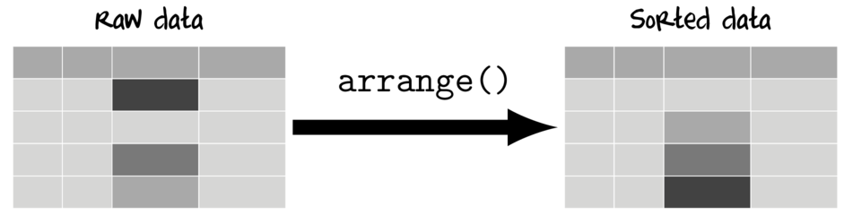
Most statistical analyses are invariant to the data order and thus data reordering is typically only for aesthetics in tables and figures.
Sorting data has the potential to be one of the most dangerous forms of data manipulation - particularly in spreadsheets in which there is no real binding between individual columns or rows. It is far to easy to accidentally sort the data in a single column (or row) without applying the ordering to all the other columns in the data set thereby resulting in broken data.
Whilst the above apocalypse is still possible in R, the data structures and manipulation interfaces mean that you really have to try to break the data in this way. Furthermore, you are encouraged to store reordered data in a different object to the original data, and hence 'rolling' back is trivial.
| An example of an data set (data.1) | |||||||||||||||||||||||||||||||||||||||||||||||||||||||||||||||||||||||||||||||||||||||||||||
|---|---|---|---|---|---|---|---|---|---|---|---|---|---|---|---|---|---|---|---|---|---|---|---|---|---|---|---|---|---|---|---|---|---|---|---|---|---|---|---|---|---|---|---|---|---|---|---|---|---|---|---|---|---|---|---|---|---|---|---|---|---|---|---|---|---|---|---|---|---|---|---|---|---|---|---|---|---|---|---|---|---|---|---|---|---|---|---|---|---|---|---|---|---|
|
|
| Sort the data by LAT |
|---|
|
|
| Sort the data by LAT (highest to lowest) |
|---|
|
|
| Sort the data by Cond and then Temp |
|---|
|
|
| Sort the data by the sum of Temp and LAT |
|---|
|
|
Re-levelling (sorting) factors
In the previous section, we altered the order of the records in the data set. However, it is important to realize that categorical variables in a dataframe have a property (called levels) that indicates the order of the levels of the factor and that this property is completely independent of the order of records in the data structure. By default, categorical variables (factors) are ordered alphabetically (as I said, irrespective of their order in the data set). The order of factor levels dictates the order in which groups will be plotted in figures and tabulated in tables. Consequently, re-levelling factors is often desirable
| An example of an data set (data.2) | |||||||||||||||||||||||||||||||||||||||||||||||||||||||||||||||||||||||
|---|---|---|---|---|---|---|---|---|---|---|---|---|---|---|---|---|---|---|---|---|---|---|---|---|---|---|---|---|---|---|---|---|---|---|---|---|---|---|---|---|---|---|---|---|---|---|---|---|---|---|---|---|---|---|---|---|---|---|---|---|---|---|---|---|---|---|---|---|---|---|---|
|
|
Sometimes it is useful (particularly when preparing data for graphing) to have the order of the levels of a factor defined by another variable - for example to allow groups to be plotted from highest to lowest response etc. This can be achieved via the fct_reorder() and fct_reorder2() functions from the forcats package.
| An example of an data set (data.2) | |||||||||||||||||||||||||||||||||||||||||||||||||||||||||||||||||||||||
|---|---|---|---|---|---|---|---|---|---|---|---|---|---|---|---|---|---|---|---|---|---|---|---|---|---|---|---|---|---|---|---|---|---|---|---|---|---|---|---|---|---|---|---|---|---|---|---|---|---|---|---|---|---|---|---|---|---|---|---|---|---|---|---|---|---|---|---|---|---|---|---|
|
|
Relabelling a factor
In this case, the L,M,H labels are efficient, yet not as informative as we would perhaps like for labels on a graphic. Instead, we would probably prefer they were something like, "Low", "Medium" and "High"
| Give the levels of a factor more informative labels |
|---|
|
Renaming columns (variables)
Data can be sourced from a variety of locations and often the column (=variable or field names) are either non-informative, very long or otherwise not convenient. It is possible to rename any or all of the column names of a data frame (or matrix).
| Rename the column names (variables) |
|---|
|
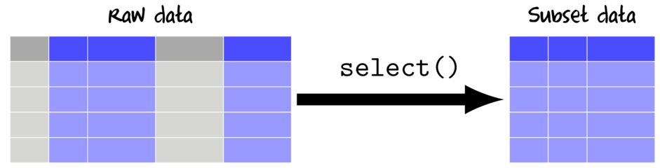
Subsetting
We regularly want to run an analysis or generate a graphic for a sub-set of the data. Take for example the data used here. We may, for example, wish to explore a subset of the data for which Cond is "H". Warning, following any subsetting, it is crucial that you then instruct R to redefine the factor levels of any factors in the subsetted data set. When subsetting a dataset, all factors simply inherit the original levels property of the original factors, and therefore the new factors potentially define more factor levels than are in the actually present in the subsetted data set. This, along with the solution is illustrated below.
Another form of subsetting is where we wish to reduce the number of columns of the data frame to remove excessive and unwanted data fields. The two forms of subsetting are thus:
- reducing the number of rows - filtering
- reducing the number of columns - selecting
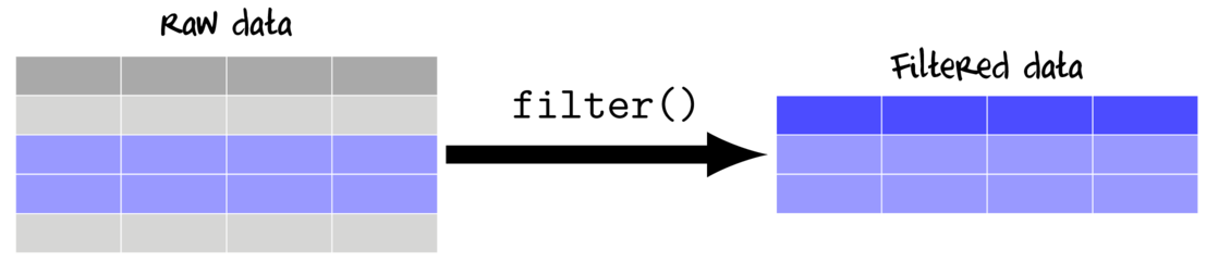
Filtering (subsetting by rows)
Filtering selects rows for which a condition is evaluated to be TRUE. Hence, any logical expression or vectorized function that returns Boolean values (TRUE or FALSE) can be used for filtering.
| An example of a data set (data.2) | ||||||||||||||||||||||||||||||||||||||||||||||||||||||||||||||||||
|---|---|---|---|---|---|---|---|---|---|---|---|---|---|---|---|---|---|---|---|---|---|---|---|---|---|---|---|---|---|---|---|---|---|---|---|---|---|---|---|---|---|---|---|---|---|---|---|---|---|---|---|---|---|---|---|---|---|---|---|---|---|---|---|---|---|---|
|
View code
set.seed(1) data.2 <- expand.grid(Plot=paste("P",1:4,sep=""),Cond=c("H","M","L")) data.2$Cond <- factor(as.character(data.2$Cond)) data.2$Between <- gl(4,3,12,lab=paste("A",1:4,sep="")) data.2$Temp <- rnorm(12,22,10) |
| Keep only the observations where Cond is H |
|---|
|
Via filter (package:dplyr)
data.2 %>% filter(Cond=="H") Plot Cond Between Temp 1 P1 H A1 15.73546 2 P2 H A1 23.83643 3 P3 H A1 13.64371 4 P4 H A2 37.95281 Via subset
subset(data.2,Cond=="H") Plot Cond Between Temp 1 P1 H A1 15.73546 2 P2 H A1 23.83643 3 P3 H A1 13.64371 4 P4 H A2 37.95281 Via indexing
data.2[data.2$Cond=="H",] Plot Cond Between Temp 1 P1 H A1 15.73546 2 P2 H A1 23.83643 3 P3 H A1 13.64371 4 P4 H A2 37.95281 |
| Keep only the observations for which Temp is between 15 and 20 |
|---|
|
Via filter (package:dplyr)
data.2 %>% filter(between(Temp,15,20)) Plot Cond Between Temp 1 P1 H A1 15.73546 2 P2 L A4 18.94612 Via subset
subset(data.2, Temp>15 & Temp<20) Plot Cond Between Temp 1 P1 H A1 15.73546 10 P2 L A4 18.94612 Via indexing
data.2[data.2$Temp>15 & data.2$Temp<20,] Plot Cond Between Temp 1 P1 H A1 15.73546 10 P2 L A4 18.94612 |
| Keep only the observations after Temp has surpassed 25 |
|---|
|
Via filter (package:dplyr)
data.2 %>% filter(cumany(Temp>25)) Plot Cond Between Temp 1 P4 H A2 37.95281 2 P1 M A2 25.29508 3 P2 M A2 13.79532 4 P3 M A3 26.87429 5 P4 M A3 29.38325 6 P1 L A3 27.75781 7 P2 L A4 18.94612 8 P3 L A4 37.11781 9 P4 L A4 25.89843 |
| Keep only the observations where Cond is either H or M |
|---|
|
Via filter (package:dplyr)
filter(data.2,Cond %in% c("H","M"))
#OR
filter(data.2,Cond=="H" | Cond=="M")
Plot Cond Between Temp 1 P1 H A1 15.73546 2 P2 H A1 23.83643 3 P3 H A1 13.64371 4 P4 H A2 37.95281 5 P1 M A2 25.29508 6 P2 M A2 13.79532 7 P3 M A3 26.87429 8 P4 M A3 29.38325 Via subset
subset(data.2,Cond %in% c("H","M")) Plot Cond Between Temp 1 P1 H A1 15.73546 2 P2 H A1 23.83643 3 P3 H A1 13.64371 4 P4 H A2 37.95281 5 P1 M A2 25.29508 6 P2 M A2 13.79532 7 P3 M A3 26.87429 8 P4 M A3 29.38325 Via indexing
data.2[data.2$Cond %in% c("H","M"),] Plot Cond Between Temp 1 P1 H A1 15.73546 2 P2 H A1 23.83643 3 P3 H A1 13.64371 4 P4 H A2 37.95281 5 P1 M A2 25.29508 6 P2 M A2 13.79532 7 P3 M A3 26.87429 8 P4 M A3 29.38325 |
| Keep only the observations with H OR M condition AND Temp < 30 |
|---|
|
Via filter (package:dplyr)
filter(data.2,Cond %in% c("H","M") & Temp<30)
#OR
filter(data.2,Cond %in% c("H","M"), Temp<30)
Plot Cond Between Temp 1 P1 H A1 15.73546 2 P2 H A1 23.83643 3 P3 H A1 13.64371 4 P1 M A2 25.29508 5 P2 M A2 13.79532 6 P3 M A3 26.87429 7 P4 M A3 29.38325 Via subset
subset(data.2,Cond %in% c("H","M") & Temp<30) Plot Cond Between Temp 1 P1 H A1 15.73546 2 P2 H A1 23.83643 3 P3 H A1 13.64371 5 P1 M A2 25.29508 6 P2 M A2 13.79532 7 P3 M A3 26.87429 8 P4 M A3 29.38325 Via indexing
#Note, the following will yield unexpected results when there are missing values!
data.2[data.2$Cond %in% c("H","M") & data.2$Temp<30,]
Plot Cond Between Temp 1 P1 H A1 15.73546 2 P2 H A1 23.83643 3 P3 H A1 13.64371 5 P1 M A2 25.29508 6 P2 M A2 13.79532 7 P3 M A3 26.87429 8 P4 M A3 29.38325 |
| Keep only the observations with Cond of H and Temp < 30 OR Cond of M and Temp < 26 |
|---|
- (Cond=="H" & Temp<30) | (Cond=='M' & Temp<26)
- (Cond=="H") & (Temp<30 | Cond=='M') & Temp<26)
- (Cond=="H") & (Temp<30 | Cond=='M' & Temp<26)
- (Cond=="H" & (Temp<30 | Cond=='M')) & Temp<26
- ...
|
Via filter (package:dplyr)
filter(data.2,(Cond=="H" & Temp<30) | (Cond=='M' & Temp<26)) Plot Cond Between Temp 1 P1 H A1 15.73546 2 P2 H A1 23.83643 3 P3 H A1 13.64371 4 P1 M A2 25.29508 5 P2 M A2 13.79532 Via subset
subset(data.2,(Cond=="H" & Temp<30) | (Cond=='M' & Temp<26)) Plot Cond Between Temp 1 P1 H A1 15.73546 2 P2 H A1 23.83643 3 P3 H A1 13.64371 5 P1 M A2 25.29508 6 P2 M A2 13.79532 Via indexing
#Note, the following will yield unexpected results when there are missing values!
data.2[(data.2$Cond=="H" & data.2$Temp<30) | (data.2$Cond=='M' & data.2$Temp<26),]
Plot Cond Between Temp 1 P1 H A1 15.73546 2 P2 H A1 23.83643 3 P3 H A1 13.64371 5 P1 M A2 25.29508 6 P2 M A2 13.79532 |
| Effect of subsetting on factor levels |
|---|
#examine the levels of the Cond factor
levels(data.2$Cond)
[1] "H" "L" "M" #subset the dataset to just Cond H data.3<-filter(data.2,Cond=="H") #examine subset data data.3 Plot Cond Between Temp 1 P1 H A1 15.73546 2 P2 H A1 23.83643 3 P3 H A1 13.64371 4 P4 H A2 37.95281 #examine the levels of the Cond factor levels(data.3$Cond) [1] "H" "L" "M" levels(data.3$Between) [1] "A1" "A2" "A3" "A4" |
Notice that although we created a subset of the data that only includes cases where Cond is "H", each of the factors have retained their original level properties. |
| Correcting factor levels of all factors after subsetting |
|---|
#subset the dataset to just Cond H
data.3<-filter(data.2,Cond=="H")
#drop the unused factor levels from all factors
data.3<-droplevels(data.3)
#examine the levels of each factor
levels(data.3$Cond)
[1] "H" levels(data.3$Between) [1] "A1" "A2" |
Notice this time, the levels of each factor reflect the subset data. |
| Correcting factor levels of only a single factor after subsetting |
|---|
#subset the dataset to just Cond H
data.3<-filter(data.2,Cond=="H")
#drop the unused factor levels from Cond
data.3$Cond<-fct_drop(data.3$Cond)
#OR
data.3$Cond<-factor(data.3$Cond)
#examine the levels of each factor
levels(data.3$Cond)
[1] "H" levels(data.3$Between) [1] "A1" "A2" "A3" "A4" |
Notice this time, the levels of the Cond factor reflect the subset data, whereas the levels of the Between factor reflect the original dataset. |
Selecting (subsetting by columns)
Selecting works by either including (or excluding) the column names that you indicate or by special 'Helper' functions that pass a vector of column indices to include in the subset data.
When selecting with the select function from the dplyr package, there are a number of "Helper" functions that provide convenient ways to select columns:
- contains(""), columns whose name match the character string (not case sensitive by default)
- starts_with(""), columns whose names begin with the character string (not case sensitive by default)
- ends_with(""), columns whose names end with the character string (not case sensitive by default)
- one_of(c("","")), columns whose names are amongst the character strings
- matches(""), columns whose names are matched by the character string of a regular expression (not case sensitive by default)
- everything(), all columns. This is useful in combination with other specifiers
- num_range("",), select all columns whose names start with the first argument (a character string) followed by a number in the integer sequence provided as the second argument
| An example of a data set (data) | ||||||||||||||||||||||||||||||||||||||||||||||||||||||||||||||||||||||||||||||||||||||||||||||||||||||||||||||||||||||||||||||||||||||||||||||||||||||||||||||||||||||||||||||||
|---|---|---|---|---|---|---|---|---|---|---|---|---|---|---|---|---|---|---|---|---|---|---|---|---|---|---|---|---|---|---|---|---|---|---|---|---|---|---|---|---|---|---|---|---|---|---|---|---|---|---|---|---|---|---|---|---|---|---|---|---|---|---|---|---|---|---|---|---|---|---|---|---|---|---|---|---|---|---|---|---|---|---|---|---|---|---|---|---|---|---|---|---|---|---|---|---|---|---|---|---|---|---|---|---|---|---|---|---|---|---|---|---|---|---|---|---|---|---|---|---|---|---|---|---|---|---|---|---|---|---|---|---|---|---|---|---|---|---|---|---|---|---|---|---|---|---|---|---|---|---|---|---|---|---|---|---|---|---|---|---|---|---|---|---|---|---|---|---|---|---|---|---|---|---|---|---|
|
View code
set.seed(1) data <- expand.grid(Within=paste("B",1:2,sep=""), Subplot=paste("S",1:2,sep=""), Plot=paste("P",1:6,sep="")) data$Subplot <- gl(12,2,24,lab=paste("S",1:12,sep="")) data$Between <- gl(3,4,24,lab=paste("A",1:3,sep="")) data$Resp1 <- rpois(24,10) data$Resp2 <- rpois(24,20) data <- with(data,data.frame(Resp1,Resp2,Between,Plot,Subplot,Within)) |
| Keep only the Plot and Resp1 columns |
|---|
|
Via select (package:dplyr)
data %>% select(Plot,Resp1)
#OR
data %>% select(starts_with('Pl'),ends_with("p1"))
#OR
data %>% select(contains('Plo', ignore.case=FALSE),matches(".*p1"))
#OR
data %>% select(-matches('w.*n'),-starts_with("Sub"),-matches('Resp'),matches('Resp1'))
#OR
data %>% select(one_of(c('Plot','Resp1')))
Plot Resp1 1 P1 8 2 P1 10 3 P1 7 4 P1 11 5 P2 14 6 P2 12 7 P2 11 8 P2 9 9 P3 14 10 P3 11 11 P3 8 12 P3 2 13 P4 8 14 P4 10 15 P4 7 16 P4 12 17 P5 11 18 P5 12 19 P5 12 20 P5 10 21 P6 3 22 P6 11 23 P6 13 24 P6 7 Via subset
subset(data,select=c(Plot,Resp1)) Plot Resp1 1 P1 8 2 P1 10 3 P1 7 4 P1 11 5 P2 14 6 P2 12 7 P2 11 8 P2 9 9 P3 14 10 P3 11 11 P3 8 12 P3 2 13 P4 8 14 P4 10 15 P4 7 16 P4 12 17 P5 11 18 P5 12 19 P5 12 20 P5 10 21 P6 3 22 P6 11 23 P6 13 24 P6 7 #OR subset(data,select=c("Plot","Resp1")) Plot Resp1 1 P1 8 2 P1 10 3 P1 7 4 P1 11 5 P2 14 6 P2 12 7 P2 11 8 P2 9 9 P3 14 10 P3 11 11 P3 8 12 P3 2 13 P4 8 14 P4 10 15 P4 7 16 P4 12 17 P5 11 18 P5 12 19 P5 12 20 P5 10 21 P6 3 22 P6 11 23 P6 13 24 P6 7 Via indexing
data[,c("Plot","Resp1")] Plot Resp1 1 P1 8 2 P1 10 3 P1 7 4 P1 11 5 P2 14 6 P2 12 7 P2 11 8 P2 9 9 P3 14 10 P3 11 11 P3 8 12 P3 2 13 P4 8 14 P4 10 15 P4 7 16 P4 12 17 P5 11 18 P5 12 19 P5 12 20 P5 10 21 P6 3 22 P6 11 23 P6 13 24 P6 7 |
| Keep the Plot/Subplot and Resp columns only |
|---|
|
Via select (package:dplyr)
data %>% select(Plot,Subplot,Resp1,Resp2)
#OR
data %>% select(contains('plot'), matches('^Resp.*'))
#OR
data %>% select(matches('plot$'), num_range('Resp',1:2))
#OR
data %>% select(contains('plot'),everything(),-matches('w.*n'))
Plot Subplot Resp1 Resp2 1 P1 S1 8 17 2 P1 S1 10 18 3 P1 S2 7 17 4 P1 S2 11 21 5 P2 S3 14 19 6 P2 S3 12 13 7 P2 S4 11 24 8 P2 S4 9 18 9 P3 S5 14 25 10 P3 S5 11 18 11 P3 S6 8 27 12 P3 S6 2 22 13 P4 S7 8 17 14 P4 S7 10 22 15 P4 S8 7 16 16 P4 S8 12 13 17 P5 S9 11 23 18 P5 S9 12 19 19 P5 S10 12 23 20 P5 S10 10 21 21 P6 S11 3 17 22 P6 S11 11 16 23 P6 S12 13 26 24 P6 S12 7 28 Via subset
subset(data,select=c(Plot,Subplot,Resp1,Resp2)) Plot Subplot Resp1 Resp2 1 P1 S1 8 17 2 P1 S1 10 18 3 P1 S2 7 17 4 P1 S2 11 21 5 P2 S3 14 19 6 P2 S3 12 13 7 P2 S4 11 24 8 P2 S4 9 18 9 P3 S5 14 25 10 P3 S5 11 18 11 P3 S6 8 27 12 P3 S6 2 22 13 P4 S7 8 17 14 P4 S7 10 22 15 P4 S8 7 16 16 P4 S8 12 13 17 P5 S9 11 23 18 P5 S9 12 19 19 P5 S10 12 23 20 P5 S10 10 21 21 P6 S11 3 17 22 P6 S11 11 16 23 P6 S12 13 26 24 P6 S12 7 28 #OR subset(data,select=c("Plot","Subplot","Resp1","Resp2")) Plot Subplot Resp1 Resp2 1 P1 S1 8 17 2 P1 S1 10 18 3 P1 S2 7 17 4 P1 S2 11 21 5 P2 S3 14 19 6 P2 S3 12 13 7 P2 S4 11 24 8 P2 S4 9 18 9 P3 S5 14 25 10 P3 S5 11 18 11 P3 S6 8 27 12 P3 S6 2 22 13 P4 S7 8 17 14 P4 S7 10 22 15 P4 S8 7 16 16 P4 S8 12 13 17 P5 S9 11 23 18 P5 S9 12 19 19 P5 S10 12 23 20 P5 S10 10 21 21 P6 S11 3 17 22 P6 S11 11 16 23 P6 S12 13 26 24 P6 S12 7 28 Via indexing
data[,c("Plot","Subplot","Resp1","Resp2")] Plot Subplot Resp1 Resp2 1 P1 S1 8 17 2 P1 S1 10 18 3 P1 S2 7 17 4 P1 S2 11 21 5 P2 S3 14 19 6 P2 S3 12 13 7 P2 S4 11 24 8 P2 S4 9 18 9 P3 S5 14 25 10 P3 S5 11 18 11 P3 S6 8 27 12 P3 S6 2 22 13 P4 S7 8 17 14 P4 S7 10 22 15 P4 S8 7 16 16 P4 S8 12 13 17 P5 S9 11 23 18 P5 S9 12 19 19 P5 S10 12 23 20 P5 S10 10 21 21 P6 S11 3 17 22 P6 S11 11 16 23 P6 S12 13 26 24 P6 S12 7 28 |
select_if
There is also a special form of select that selects if a condition is satisfied.
| Keep only the numeric variables |
|---|
|
Via select (package:dplyr)
data %>% select_if(is.numeric) |
filter and select
Recall that one of the advantages of working within the grammar of data manipulation framework is that data can be piped from one tool to another to achieve multiple manipulations.
| Keep only the Plot and Temp columns and observations with H OR M condition AND Temp < 30 |
|---|
|
Via filter and select (package:dplyr)
data.2 %>% filter(Cond %in% c("H","M") & Temp<30) %>% select(Plot, Temp) Plot Temp 1 P1 15.73546 2 P2 23.83643 3 P3 13.64371 4 P1 25.29508 5 P2 13.79532 6 P3 26.87429 7 P4 29.38325 Via subset
subset(data.2,Cond %in% c("H","M") & Temp<30, select=c(Plot,Temp)) Plot Temp 1 P1 15.73546 2 P2 23.83643 3 P3 13.64371 5 P1 25.29508 6 P2 13.79532 7 P3 26.87429 8 P4 29.38325 #OR subset(data.2,Cond %in% c("H","M") & Temp<30, select=c(-Cond,-Between)) Plot Temp 1 P1 15.73546 2 P2 23.83643 3 P3 13.64371 5 P1 25.29508 6 P2 13.79532 7 P3 26.87429 8 P4 29.38325 Via indexing
#Note, the following will yield unexpected results when there are missing values!
data.2[data.2$Cond %in% c("H","M") & data.2$Temp<30, c("Plot","Temp")]
Plot Temp 1 P1 15.73546 2 P2 23.83643 3 P3 13.64371 5 P1 25.29508 6 P2 13.79532 7 P3 26.87429 8 P4 29.38325 |
Adding new variables (mutating)
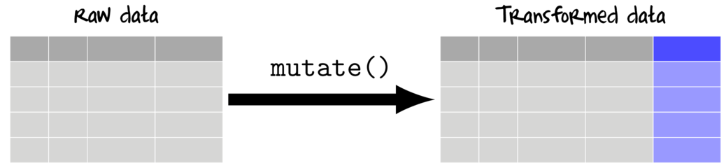
To add to (mutate) a data set, a vectorized function is applied either once or across one or more existing columns.
This section will make use of the following data set:
| A very simple dataset (data.s) | ||||||||||||||||||||||||||
|---|---|---|---|---|---|---|---|---|---|---|---|---|---|---|---|---|---|---|---|---|---|---|---|---|---|---|
|
View code
set.seed(1) data.s <- expand.grid(Plot=paste("P",1:4,sep="")) data.s$Between <- gl(2,2,4,lab=paste("A",1:2,sep="")) data.s <- with(data.s,data.frame(Between,Plot,Resp1=rpois(4,10), Resp2=rpois(4,20))) |
Whether transforming/scaling existing variables or generating new variables derived from existing variables it is advisable that existing variables be retained (unless the data are huge and storage is tight). As with other routines featured in this tutorial, there are numerous ways to derive new variables from existing variables. The main options;
data.s$logResp1 <- log(data.s$Resp1)
data.s$logResp2 <- log(data.s$Resp2)
data.s
  Between Plot Resp1 Resp2 logResp1 logResp2
1      A1   P1     8    13 2.079442 2.564949
2      A1   P2    10    22 2.302585 3.091042
3      A2   P3     7    23 1.945910 3.135494
4      A2   P4    11    22 2.397895 3.091042
transform(data.s, logResp1=log(Resp1), logRes2=log(Resp2))
  Between Plot Resp1 Resp2 logResp1  logRes2
1      A1   P1     8    13 2.079442 2.564949
2      A1   P2    10    22 2.302585 3.091042
3      A2   P3     7    23 1.945910 3.135494
4      A2   P4    11    22 2.397895 3.091042
data.s
  Between Plot Resp1 Resp2
1      A1   P1     8    13
2      A1   P2    10    22
3      A2   P3     7    23
4      A2   P4    11    22
data.s %>% mutate(logResp1=log(Resp1), logRes2=log(Resp2))
  Between Plot Resp1 Resp2 logResp1  logRes2
1      A1   P1     8    13 2.079442 2.564949
2      A1   P2    10    22 2.302585 3.091042
3      A2   P3     7    23 1.945910 3.135494
4      A2   P4    11    22 2.397895 3.091042
data.s
  Between Plot Resp1 Resp2
1      A1   P1     8    13
2      A1   P2    10    22
3      A2   P3     7    23
4      A2   P4    11    22
The main features of each of the above functions are compared and contrasted in the following table.
| Transforms at a time | Returns | Notes | |
|---|---|---|---|
| manually | Single | Single vectors | |
| transform | Multiple | New dataframe | Somewhat similar to within(). |
| mutate | Multiple | New dataframe | Works with each column sequentially and therefore can derive new columns using the columns created in earlier iterations. |
| Scale (log) transform a single variable - Resp1 |
|---|
|
Via mutate
data.s %>% mutate(logResp1=log(Resp1)) Between Plot Resp1 Resp2 logResp1 1 A1 P1 8 13 2.079442 2 A1 P2 10 22 2.302585 3 A2 P3 7 23 1.945910 4 A2 P4 11 22 2.397895 Via transform
transform(data.s,logResp1=log(Resp1)) Between Plot Resp1 Resp2 logResp1 1 A1 P1 8 13 2.079442 2 A1 P2 10 22 2.302585 3 A2 P3 7 23 1.945910 4 A2 P4 11 22 2.397895 |
| Scale (log) transform a multiple variables (Resp1 and Resp2) and then calculate the difference |
|---|
|
Via mutate
data.s %>% mutate(logResp1=log(Resp1), logResp2=log(Resp2), Diff=logResp2-logResp1) Between Plot Resp1 Resp2 logResp1 logResp2 Diff 1 A1 P1 8 13 2.079442 2.564949 0.4855078 2 A1 P2 10 22 2.302585 3.091042 0.7884574 3 A2 P3 7 23 1.945910 3.135494 1.1895841 4 A2 P4 11 22 2.397895 3.091042 0.6931472 Via transform
tmp=transform(data.s,logResp1=log(Resp1), logResp2=log(Resp2))
transform(tmp, Diff=logResp2-logResp1)
Between Plot Resp1 Resp2 logResp1 logResp2 Diff 1 A1 P1 8 13 2.079442 2.564949 0.4855078 2 A1 P2 10 22 2.302585 3.091042 0.7884574 3 A2 P3 7 23 1.945910 3.135494 1.1895841 4 A2 P4 11 22 2.397895 3.091042 0.6931472 |
Vectorized functions
Recall that any function that returns a either a single value or a vector of length equal to the number of rows in the data can be used. The dplyr package also comes with a number of "Vectorized" functions for performing common data manipulation routines:
data.s %>% mutate(leadResp1=lead(Resp1), lagResp1=lag(Resp1))
  Between Plot Resp1 Resp2 leadResp1 lagResp1
1      A1   P1     8    13        10       NA
2      A1   P2    10    22         7        8
3      A2   P3     7    23        11       10
4      A2   P4    11    22        NA        7
mutate(data.s, rankResp2=rank(Resp2), drnkResp2=dense_rank(Resp2), mrnkResp2=min_rank(Resp2),
    prnkResp2=percent_rank(Resp2))
  Between Plot Resp1 Resp2 rankResp2 drnkResp2 mrnkResp2 prnkResp2
1      A1   P1     8    13       1.0         1         1 0.0000000
2      A1   P2    10    22       2.5         2         2 0.3333333
3      A2   P3     7    23       4.0         3         4 1.0000000
4      A2   P4    11    22       2.5         2         2 0.3333333
mutate(data.s, tileResp1=ntile(Resp1,3), btwnResp1=between(Resp1,9,12))
  Between Plot Resp1 Resp2 tileResp1 btwnResp1
1      A1   P1     8    13         1     FALSE
2      A1   P2    10    22         2      TRUE
3      A2   P3     7    23         1     FALSE
4      A2   P4    11    22         3      TRUE
## Cummulative distribution
data.s %>% mutate(csResp1=cumsum(Resp1), cdResp1=cume_dist(Resp1))
  Between Plot Resp1 Resp2 csResp1 cdResp1
1      A1   P1     8    13       8    0.50
2      A1   P2    10    22      18    0.75
3      A2   P3     7    23      25    0.25
4      A2   P4    11    22      36    1.00
## Predicates of cummulatives.
## Accumulate only those that have a Resp1 > 9
## Accumulate only if all have a Resp1 > 7
data.s %>% mutate(csResp1=cumsum(Resp1), cnyResp1=cumany(Resp1>9), callResp1=cumall(Resp1>7))
  Between Plot Resp1 Resp2 csResp1 cnyResp1 callResp1
1      A1   P1     8    13       8    FALSE      TRUE
2      A1   P2    10    22      18     TRUE      TRUE
3      A2   P3     7    23      25     TRUE     FALSE
4      A2   P4    11    22      36     TRUE     FALSE
## The above window functions are useful for filtering
data.s %>% filter(cumall(Resp1>7))
  Between Plot Resp1 Resp2
1      A1   P1     8    13
2      A1   P2    10    22
## Cumulative product and mean
data.s %>% mutate(cpResp1=cumprod(Resp1), cmResp1=cummean(Resp1))
  Between Plot Resp1 Resp2 cpResp1  cmResp1
1      A1   P1     8    13       8 8.000000
2      A1   P2    10    22      80 9.000000
3      A2   P3     7    23     560 8.333333
4      A2   P4    11    22    6160 9.000000
## Cumulative min and max
data.s %>% mutate(cminResp1=cummin(Resp1), cmaxResp1=cummax(Resp1))
  Between Plot Resp1 Resp2 cminResp1 cmaxResp1
1      A1   P1     8    13         8         8
2      A1   P2    10    22         8        10
3      A2   P3     7    23         7        10
4      A2   P4    11    22         7        11
The extended mutate_ family
In addition to the mutate() function, the dplyr package also has a number of alternative mutate_ functons that provide convenient ways to select which columns to apply functions to.
- mutate_all(), apply function(s) to all columns
- mutate_at(), apply function(s) to selected columns
- mutate_if(), apply function(s) to columns that satisfy a specific condition
| Scale (log) transform multiple variables - Resp1 and Resp2 |
|---|
|
Via mutate
data.s %>% mutate(Resp1_log=log(Resp1),Resp2_log=log(Resp2))
#OR to account for any number of transformations
data.s %>% mutate_at(vars(Resp1,Resp2), funs(log=log))
#OR
data.s %>% mutate_at(vars(contains("Resp")), funs(log=log))
#OR
data.s %>% mutate_if(is.numeric, funs(log=log))
Between Plot Resp1 Resp2 Resp1_log Resp2_log 1 A1 P1 8 13 2.079442 2.564949 2 A1 P2 10 22 2.302585 3.091042 3 A2 P3 7 23 1.945910 3.135494 4 A2 P4 11 22 2.397895 3.091042 Via transform
transform(data.s,Resp1_log=log(Resp1),Resp2_log=log(Resp2)) Between Plot Resp1 Resp2 Resp1_log Resp2_log 1 A1 P1 8 13 2.079442 2.564949 2 A1 P2 10 22 2.302585 3.091042 3 A2 P3 7 23 1.945910 3.135494 4 A2 P4 11 22 2.397895 3.091042 |
| Apply a summary function to convert all character vectors into lowercase |
|---|
|
Via mutate
mutate_if(data.s, is.character, stringr:::str_to_lower) Between Plot Resp1 Resp2 1 a1 p1 8 13 2 a1 p2 10 22 3 a2 p3 7 23 4 a2 p4 11 22 |
| Applying multiple functions to multiple variables |
|---|
|
Via mutate
mutate_at(data.s, vars(contains('Resp')), funs(log=log, c=scale(.,scale=FALSE)))
#OR
mutate_at(data.s, vars(Resp1,Resp2), funs(log=log, c=.-mean(.)))
Between Plot Resp1 Resp2 Resp1_log Resp2_log Resp1_c Resp2_c 1 A1 P1 8 13 2.079442 2.564949 -1 -7 2 A1 P2 10 22 2.302585 3.091042 1 2 3 A2 P3 7 23 1.945910 3.135494 -2 3 4 A2 P4 11 22 2.397895 3.091042 2 2 |
| Apply a summary function to multiple variables - Resp1 and Resp2 |
|---|
|
Via mutate
mutate(data.s,Resp1_mean=mean(Resp1, na.rm=TRUE),Resp2_mean=mean(Resp2, na.rm=TRUE))
#OR
mutate_at(data.s, vars(Resp1,Resp2),funs(mean=mean(.,na.rm=TRUE)))
Between Plot Resp1 Resp2 Resp1_mean Resp2_mean 1 A1 P1 8 13 9 20 2 A1 P2 10 22 9 20 3 A2 P3 7 23 9 20 4 A2 P4 11 22 9 20 Via transform
transform(data.s,mutate(data.s,Resp1_mean=mean(Resp1, na.rm=TRUE),Resp2_mean=mean(Resp2, na.rm=TRUE))) Between Plot Resp1 Resp2 1 A1 P1 8 13 2 A1 P2 10 22 3 A2 P3 7 23 4 A2 P4 11 22 |
Summarizing (aggregating) data
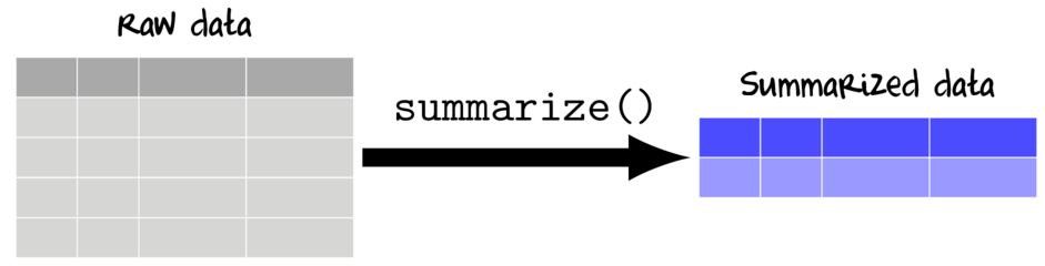
Data are often collected and transcribed at finer temporal/spatial scales and with greater fidelity than is required for all analyses. Therefore an important phase of data preparation is also to summarize the data into the spatial/temporal scales appropriate for the desired graphical and statistical analyses.
Summarizing involves applying one or more summarizing functions to one or more variables.
| An example of a data set (data) | ||||||||||||||||||||||||||||||||||||||||||||||||||||||||||||||||||||||||||||||||||||||||||||||||||||||||||||||||||||||||||||||||||||||||||||||||||||||||||||||||||||||||||||||||
|---|---|---|---|---|---|---|---|---|---|---|---|---|---|---|---|---|---|---|---|---|---|---|---|---|---|---|---|---|---|---|---|---|---|---|---|---|---|---|---|---|---|---|---|---|---|---|---|---|---|---|---|---|---|---|---|---|---|---|---|---|---|---|---|---|---|---|---|---|---|---|---|---|---|---|---|---|---|---|---|---|---|---|---|---|---|---|---|---|---|---|---|---|---|---|---|---|---|---|---|---|---|---|---|---|---|---|---|---|---|---|---|---|---|---|---|---|---|---|---|---|---|---|---|---|---|---|---|---|---|---|---|---|---|---|---|---|---|---|---|---|---|---|---|---|---|---|---|---|---|---|---|---|---|---|---|---|---|---|---|---|---|---|---|---|---|---|---|---|---|---|---|---|---|---|---|---|
|
View code
set.seed(1) data <- expand.grid(Within=paste("B",1:2,sep=""), Subplot=paste("S",1:2,sep=""), Plot=paste("P",1:6,sep="")) data$Subplot <- gl(12,2,24,lab=paste("S",1:12,sep="")) data$Between <- gl(3,4,24,lab=paste("A",1:3,sep="")) data$Resp1 <- rpois(24,10) data$Resp2 <- rpois(24,20) data <- with(data,data.frame(Resp1,Resp2,Between,Plot,Subplot,Within)) |
| Calculate the mean Resp1 |
|---|
|
Via mutate
data %>% summarize(mean(Resp1)) mean(Resp1) 1 9.708333 Via code
mean(data$Resp1) [1] 9.708333 |
Note, unlike the base R solution (and consistent with all the grammar of data manipulation verbs) the dplyr pathway always yields a data.frame (actually a tibble). This is not only a data type that permits further manipulation, it is also a convenient format for producing tabular and graphical summaries.
| Calculate the mean and standard deviation of Resp1 |
|---|
|
Via mutate
data %>% summarize(mean(Resp1), sd(Resp1)) mean(Resp1) sd(Resp1) 1 9.708333 3.04287 Via code
mean(data$Resp1) [1] 9.708333 sd(data$Resp1) [1] 3.04287 |
| Calculate a range of summary statistics |
|---|
|
Via mutate
data %>% summarize(mean(Resp1), sd(Resp1), n(), n_distinct(Resp1), first(Resp1), min(Resp1), max(Resp1)) mean(Resp1) sd(Resp1) n() n_distinct(Resp1) first(Resp1) min(Resp1) max(Resp1) 1 9.708333 3.04287 24 10 8 2 14 |
| Calculate the mean of both Resp1 and Resp2 |
|---|
|
Via mutate
data %>% summarize(mean(Resp1), mean(Resp2)) mean(Resp1) mean(Resp2) 1 9.708333 20 Via code
mean(data$Resp1) [1] 9.708333 mean(data$Resp2) [1] 20 |
The extended summary_ family
As with the mutate function, the dplyr package also has a number of alternative summarize_ functons that provide convenient ways to select which columns to apply functions to.
- summarize_all(), apply function(s) to all columns
- summarize_at(), apply function(s) to selected columns
- summarize_if(), apply function(s) to columns that satisfy a specific condition
| Calculate the mean of both Resp1 and Resp2 |
|---|
|
Via mutate
data %>% summarize_at(vars(Resp1,Resp2), mean) Resp1 Resp2 1 9.708333 20 #OR data %>% summarize_if(is.numeric, mean) Resp1 Resp2 1 9.708333 20 |
| Calculate the mean and standard deviation of both Resp1 and Resp2 |
|---|
|
Via mutate
data %>% summarize_at(vars(Resp1,Resp2), funs(mean,sd)) Resp1_mean Resp2_mean Resp1_sd Resp2_sd 1 9.708333 20 3.04287 4.159849 #OR data %>% summarize_if(is.numeric, funs(mean,sd)) Resp1_mean Resp2_mean Resp1_sd Resp2_sd 1 9.708333 20 3.04287 4.159849 |
Grouping data
Base R has a family of apply functions that apply a function (such as mean()) to a continuous variable separately for:
- apply(), each column or row.
apply(data[,1:2], MARGIN=2, mean)
    Resp1     Resp2
 9.708333 20.000000
- tapply(), each level of a categorical vector (factor)
tapply(data$Resp1, data$Between, mean)
    A1     A2     A3
 9.125 11.375  8.625
Central to the modern split/apply/combine process is the idea of groups. Groups are the basis of splitting the data. Functions applied to grouped data are applied to each group (subset) separately before the results are combined back into a single data frame (actually tibble). Hence grouped data are most powerful when combined with the summarize() or mutate() families of functions.
data %>% group_by(Between)
Source: local data frame [24 x 6]
Groups: Between [3]

   Resp1 Resp2 Between   Plot Subplot Within
   <int> <int>  <fctr> <fctr>  <fctr> <fctr>
1      8    17      A1     P1      S1     B1
2     10    18      A1     P1      S1     B2
3      7    17      A1     P1      S2     B1
4     11    21      A1     P1      S2     B2
5     14    19      A2     P2      S3     B1
6     12    13      A2     P2      S3     B2
7     11    24      A2     P2      S4     B1
8      9    18      A2     P2      S4     B2
9     14    25      A3     P3      S5     B1
10    11    18      A3     P3      S5     B2
# ... with 14 more rows
Applying summarize() to grouped data
Calculate the mean and variance for Resp1 for each level of Between
data %>% group_by(Between) %>% summarize(Mean=mean(Resp1), Var=var(Resp1))
# A tibble: 3 × 3
  Between   Mean       Var
   <fctr>  <dbl>     <dbl>
1      A1  9.125  3.553571
2      A2 11.375  2.267857
3      A3  8.625 19.696429
When groups are defined, summarize() and mutate() yield tibbles. A tibble (so named because many dplyr functions generate objects with a class of tbl_df which is pronounced as 'tibble diff') is a data.frame-like object that adheres to a more strict structure (compare the following two):
# generate data.frame
data.frame('(x)'=x, A)
X.x. A 1 3.389585 b 2 7.378957 b 3 1.629561 b 4 4.778440 b 5 8.873564 a 6 5.530862 a 7 2.216495 b 8 1.581772 b 9 7.471264 b 10 5.295647 b # generate tibble data_frame('(x)'=x, A) # A tibble: 10 × 2
`(x)` A
<dbl> <chr>
1 3.389585 b
2 7.378957 b
3 1.629561 b
4 4.778440 b
5 8.873564 a
6 5.530862 a
7 2.216495 b
8 1.581772 b
9 7.471264 b
10 5.295647 b
|
# generate data.frame
data.frame('(x)'=x[1:2], A)
X.x. A 1 3.389585 b 2 7.378957 b 3 3.389585 b 4 7.378957 b 5 3.389585 a 6 7.378957 a 7 3.389585 b 8 7.378957 b 9 3.389585 b 10 7.378957 b # generate tibble data_frame('(x)'=x[1:2], A) Error: Variables must be length 1 or 10. Problem variables: '(x)' |
- variables are never auto-coerced into specific data types (e.g. character vectors are not coerced into factors)
- there are row names
- variable names are never altered (e.g. when special characters are included in names)
- only objects of length 1 are recycled
Calculate the mean and variance for Resp1 for each Between and Within combination of levels
data %>% group_by(Between,Within) %>% summarize(Mean=mean(Resp1), Var=var(Resp1))
Source: local data frame [6 x 4]
Groups: Between [?]

  Between Within  Mean        Var
   <fctr> <fctr> <dbl>      <dbl>
1      A1     B1  7.50  0.3333333
2      A1     B2 10.75  0.9166667
3      A2     B1 12.00  2.0000000
4      A2     B2 10.75  2.2500000
5      A3     B1  9.50 25.6666667
6      A3     B2  7.75 18.2500000
Calculate the mean and variance for Resp1 and Resp2 for each Between and Within combination of levels
data %>% group_by(Between,Within) %>% summarize_at(vars(Resp1,Resp2), funs(mean,var))
Source: local data frame [6 x 6]
Groups: Between [?]

  Between Within Resp1_mean Resp2_mean  Resp1_var Resp2_var
   <fctr> <fctr>      <dbl>      <dbl>      <dbl>     <dbl>
1      A1     B1       7.50      16.75  0.3333333  0.250000
2      A1     B2      10.75      18.50  0.9166667 16.333333
3      A2     B1      12.00      22.25  2.0000000  4.916667
4      A2     B2      10.75      17.75  2.2500000 11.583333
5      A3     B1       9.50      23.75 25.6666667 20.916667
6      A3     B2       7.75      21.00 18.2500000 28.000000
Hierarchical aggregations
It is useful to be able to aggregate the data to a different level of replication. Two common reasons are:- Exploratory data analysis for assessing normality, homogeneity of variance as applied to the approximate appropriate residuals (appropriate level fo replication for a give test)
- Calculating observations (typically means of subreplicates) appropriate for the desired scale of the analysis
Continuing on with the same base dataset from the previous examples, we may wish to aggregate to the level of Plots or even Subplot
Lets say that we wished to explore the distributional characteristics of Resp1 and Resp2 within each of the Between levels. The data data.frame is setup to resemble a typical hierarchical design. Notice that:
- a given Plot can only be of one Between level.
- within each Plot level there are each of the levels of within<.samp>.
- in the context of a design the Plots are the replicates of the Between factor
Generate Plot means for each of Resp1 and Resp2
data %>% group_by(Plot) %>% summarize_at(vars(Resp1,Resp2), mean)
# A tibble: 6 × 3
    Plot Resp1 Resp2
  <fctr> <dbl> <dbl>
1     P1  9.00 18.25
2     P2 11.50 18.50
3     P3  8.75 23.00
4     P4  9.25 17.00
5     P5 11.25 21.50
6     P6  8.50 21.75
The above is of limited value however as the Between variable is missing...
We can address this by including it as a group_by variable.name.
Generate Between/Plot means for each of Resp1 and Resp2
data %>% group_by(Between,Plot) %>% summarize_at(vars(Resp1,Resp2), mean)
Source: local data frame [6 x 4]
Groups: Between [?]

  Between   Plot Resp1 Resp2
   <fctr> <fctr> <dbl> <dbl>
1      A1     P1  9.00 18.25
2      A1     P4  9.25 17.00
3      A2     P2 11.50 18.50
4      A2     P5 11.25 21.50
5      A3     P3  8.75 23.00
6      A3     P6  8.50 21.75
The data design also includes a Subplot hierarchical level.
These Subplots sit under Plot in the hierarchy.
Generate Between/Plot/Subplot means for each of Resp1 and Resp2
data %>% group_by(Between,Plot,Subplot) %>% summarize_at(vars(Resp1,Resp2), mean)
Source: local data frame [12 x 5]
Groups: Between, Plot [?]

   Between   Plot Subplot Resp1 Resp2
    <fctr> <fctr>  <fctr> <dbl> <dbl>
1       A1     P1      S1   9.0  17.5
2       A1     P1      S2   9.0  19.0
3       A1     P4      S7   9.0  19.5
4       A1     P4      S8   9.5  14.5
5       A2     P2      S3  13.0  16.0
6       A2     P2      S4  10.0  21.0
7       A2     P5      S9  11.5  21.0
8       A2     P5     S10  11.0  22.0
9       A3     P3      S5  12.5  21.5
10      A3     P3      S6   5.0  24.5
11      A3     P6     S11   7.0  16.5
12      A3     P6     S12  10.0  27.0
Applying mutate() to grouped data
Grouped data are also useful in the mutate context. For example, we may wish to
center our data separately within each Plot.
Center Resp1 and Resp2 within each plot
data %>% group_by(Plot) %>% mutate_at(vars(Resp1,Resp2), funs(c=scale(.,scale=FALSE)))
Source: local data frame [24 x 8]
Groups: Plot [6]

   Resp1 Resp2 Between   Plot Subplot Within Resp1_c Resp2_c
   <int> <int>  <fctr> <fctr>  <fctr> <fctr>   <dbl>   <dbl>
1      8    17      A1     P1      S1     B1   -1.00   -1.25
2     10    18      A1     P1      S1     B2    1.00   -0.25
3      7    17      A1     P1      S2     B1   -2.00   -1.25
4     11    21      A1     P1      S2     B2    2.00    2.75
5     14    19      A2     P2      S3     B1    2.50    0.50
6     12    13      A2     P2      S3     B2    0.50   -5.50
7     11    24      A2     P2      S4     B1   -0.50    5.50
8      9    18      A2     P2      S4     B2   -2.50   -0.50
9     14    25      A3     P3      S5     B1    5.25    2.00
10    11    18      A3     P3      S5     B2    2.25   -5.00
# ... with 14 more rows
#OR
data %>% group_by(Plot) %>% mutate_at(vars(Resp1,Resp2), funs(c=. - mean(.)))
Source: local data frame [24 x 8]
Groups: Plot [6]

   Resp1 Resp2 Between   Plot Subplot Within Resp1_c Resp2_c
   <int> <int>  <fctr> <fctr>  <fctr> <fctr>   <dbl>   <dbl>
1      8    17      A1     P1      S1     B1   -1.00   -1.25
2     10    18      A1     P1      S1     B2    1.00   -0.25
3      7    17      A1     P1      S2     B1   -2.00   -1.25
4     11    21      A1     P1      S2     B2    2.00    2.75
5     14    19      A2     P2      S3     B1    2.50    0.50
6     12    13      A2     P2      S3     B2    0.50   -5.50
7     11    24      A2     P2      S4     B1   -0.50    5.50
8      9    18      A2     P2      S4     B2   -2.50   -0.50
9     14    25      A3     P3      S5     B1    5.25    2.00
10    11    18      A3     P3      S5     B2    2.25   -5.00
# ... with 14 more rows
Again, these examples could arguably be better suited to gathering first.
| Center a single variable (Resp2), centered within each level of the between variable |
|---|
|
Via ddply and transform or mutate
plyr:::ddply(data.s,~Between,transform,cResp2=Resp2-mean(Resp2)) Between Plot Resp1 Resp2 cResp2 1 A1 P1 8 13 -4.5 2 A1 P2 10 22 4.5 3 A2 P3 7 23 0.5 4 A2 P4 11 22 -0.5 #OR ddply(data.s,~Between,mutate,cResp2=Resp2-mean(Resp2)) Error in eval(expr, envir, enclos): could not find function "ddply" |
| Difference in means centered within Between (derivative of derivatives) |
|---|
|
Via ddply and mutate
plyr:::ddply(data.s,~Between,mutate,cResp1=Resp1-mean(Resp1),cResp2=Resp2-mean(Resp2),cDiff=cResp1-cResp2) Between Plot Resp1 Resp2 cResp1 cResp2 cDiff 1 A1 P1 8 13 -1 -4.5 3.5 2 A1 P2 10 22 1 4.5 -3.5 3 A2 P3 7 23 -2 0.5 -2.5 4 A2 P4 11 22 2 -0.5 2.5 |
| Scale (log) transformations of Resp1 and Resp2 centered within Between |
|---|
options(width=120)

opts_chunk$set(ts='asis',prompt=FALSE,comment=NA, fig.path='images/graphics-tut2.4', dev='my_png', fig.ext='png',warning=FALSE,message=FALSE  )

## end setup
ddply(data.s,~Between,mutate,sResp1=Resp1/max(Resp1),sResp2=Resp2/max(Resp2),logsResp1=log(sResp1),logsResp2=log(sResp2))
Error in eval(expr, envir, enclos): could not find function "ddply"
Merging (joining) data sets
It is common to have data associated with a particular study organized into a number of separate data tables (databases etc). In fact, large data sets are best managed in databases. However, statistical analyses generally require all data to be encapsulated within a single data structure. Therefore, prior to analysis, it is necessary to bring together multiple sources.
This phase of data preparation can be one of the most difficult to get right and verify.
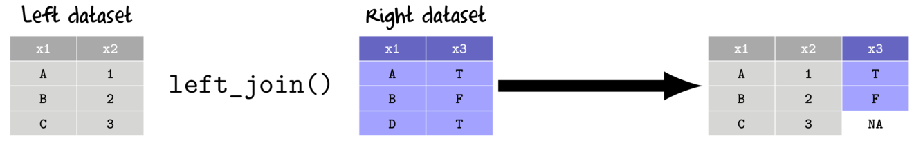
Merging (or joining) involves creating a new data set that comprises information from two data sets. The resulting joined data set contains all fields from both data sets. The data sets are alignd together according to fields they have in common. Matching records in these common fields are used to select a row from each input data set to be combined.
There are numerous alternative ways of defining what should happen in the event that common records do not occur in both sets. For example, we could specify that only fully matching records be included in the final data set. Alternatively, we could specify that all records be included from both sets and thus the resulting data set will contain missing values. The following describe these various options.
- left join
- return all rows and columns from the left data set
- return all columns from the right data set
- new columns for unmatched rows from the right data sets receive NA values
- when there are multiple matches, all combinations included
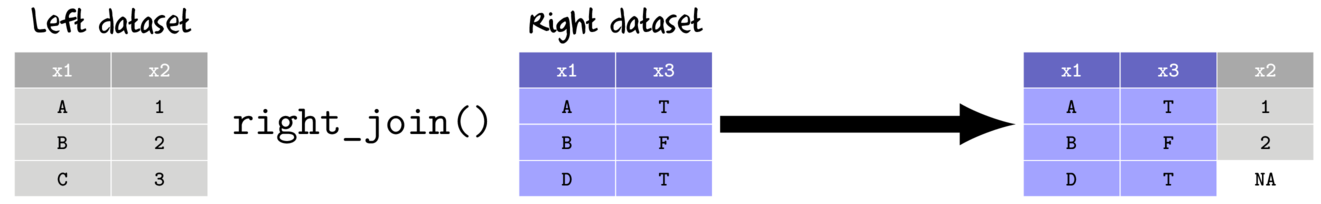
- right join
- return all rows and columns from the right data set
- return all columns from the left data set
- new columns for unmatched rows from the left data sets receive NA values
- when there are multiple matches, all combinations included
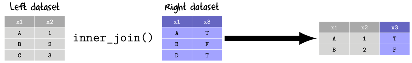
- inner join
- return all columns from the left and right data set
- return only rows that match from left and right data sets
- when there are multiple matches, all combinations included
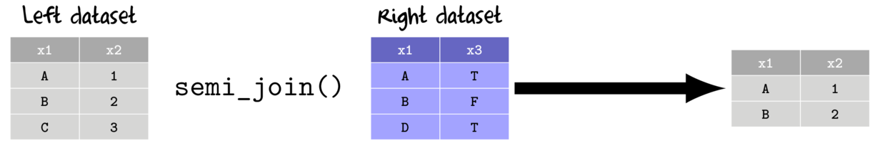
- semi join
- return all rows from the left data set that match with rows from the right data set
- keep only the columns from the left data set
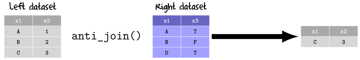
- anti join
- return only the rows from the left data set that do not match with rows from the right data set
- keep only the columns from the left data set
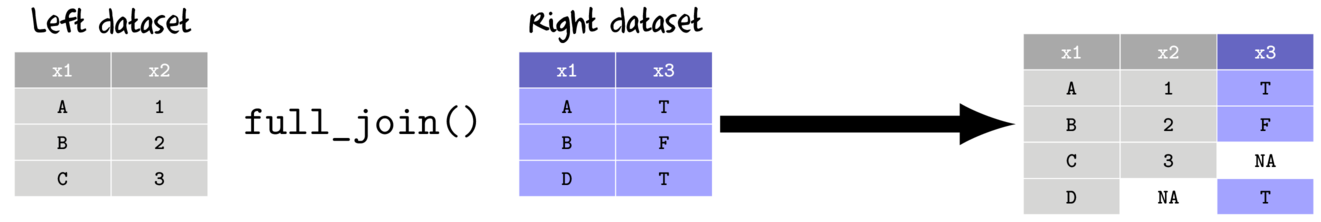
- full join
- return all rows and columns from the left and right data set
- unmatched rows from either left data sets receive NA values in the associated new columns
| Biological data set (missing Subplot 3) (data.bio) | |||||||||||||||||||||||||||||||||||||||||||||||||||||||||||||||||||||||||
|---|---|---|---|---|---|---|---|---|---|---|---|---|---|---|---|---|---|---|---|---|---|---|---|---|---|---|---|---|---|---|---|---|---|---|---|---|---|---|---|---|---|---|---|---|---|---|---|---|---|---|---|---|---|---|---|---|---|---|---|---|---|---|---|---|---|---|---|---|---|---|---|---|---|
|
View code
set.seed(1) data.bio <- expand.grid(Subplot=paste("S",1:2,sep=""),Plot=paste("P",1:6,sep="")) data.bio$Subplot <- gl(12,1,12,lab=paste("S",1:12,sep="")) data.bio$Between <- gl(3,4,12,lab=paste("A",1:3,sep="")) data.bio$Resp1 <- rpois(12,10) data.bio$Resp2 <- rpois(12,20) data.bio <- with(data.bio,data.frame(Resp1,Resp2,Between,Plot,Subplot)) data.bio<-data.bio[-3,] |
| Physio-chemical data (missing Subplot 7) (data.chem) | |||||||||||||||||||||||||||||||||||||||||||||||||||||||||||||||||||||||||
|---|---|---|---|---|---|---|---|---|---|---|---|---|---|---|---|---|---|---|---|---|---|---|---|---|---|---|---|---|---|---|---|---|---|---|---|---|---|---|---|---|---|---|---|---|---|---|---|---|---|---|---|---|---|---|---|---|---|---|---|---|---|---|---|---|---|---|---|---|---|---|---|---|---|
|
View code
set.seed(1) data.chem <- expand.grid(Subplot=paste("S",1:2,sep=""),Plot=paste("P",1:6,sep="")) data.chem$Subplot <- gl(12,1,12,lab=paste("S",1:12,sep="")) data.chem$Between <- gl(3,4,12,lab=paste("A",1:3,sep="")) data.chem$Chem1 <- rlnorm(12,1) data.chem$Chem2 <- rlnorm(12,.5) data.chem <- with(data.chem,data.frame(Chem1,Chem2,Between,Plot,Subplot)) data.chem<-data.chem[-7,] |
| Join bio and chem data (only keep full matches - an inner join) | |||||||||||||||||||||||||||||||||||||||||||||||||||||||||||||||||||||||||||||||||||||||||
|---|---|---|---|---|---|---|---|---|---|---|---|---|---|---|---|---|---|---|---|---|---|---|---|---|---|---|---|---|---|---|---|---|---|---|---|---|---|---|---|---|---|---|---|---|---|---|---|---|---|---|---|---|---|---|---|---|---|---|---|---|---|---|---|---|---|---|---|---|---|---|---|---|---|---|---|---|---|---|---|---|---|---|---|---|---|---|---|---|---|
|
Note how both Subplot 3 and 7 are absent. |
inner_join(data.bio,data.chem,by=c("Between","Plot","Subplot"))
   Resp1 Resp2 Between Plot Subplot     Chem1     Chem2
1      8    18      A1   P1      S1  1.452878 0.8858208
2     10    21      A1   P1      S2  3.266253 0.1800177
3     11    23      A1   P2      S4 13.400350 1.5762780
4     14    22      A2   P3      S5  3.779183 1.6222430
5     12    24      A2   P3      S6  1.196657 4.2369184
6      9    20      A2   P4      S8  5.687807 2.9859003
7     14    11      A3   P5      S9  4.834518 4.1328919
8     11    22      A3   P5     S10  2.002931 3.6043314
9      8    24      A3   P6     S11 12.326867 1.7763576
10     2    16      A3   P6     S12  4.014221 0.2255188
merge(data.bio,data.chem,by=c("Between","Plot","Subplot"))
   Between Plot Subplot Resp1 Resp2     Chem1     Chem2
1       A1   P1      S1     8    18  1.452878 0.8858208
2       A1   P1      S2    10    21  3.266253 0.1800177
3       A1   P2      S4    11    23 13.400350 1.5762780
4       A2   P3      S5    14    22  3.779183 1.6222430
5       A2   P3      S6    12    24  1.196657 4.2369184
6       A2   P4      S8     9    20  5.687807 2.9859003
7       A3   P5     S10    11    22  2.002931 3.6043314
8       A3   P5      S9    14    11  4.834518 4.1328919
9       A3   P6     S11     8    24 12.326867 1.7763576
10      A3   P6     S12     2    16  4.014221 0.2255188
plyr:::join(data.bio,data.chem,by=c("Between","Plot","Subplot"), type="inner")
   Resp1 Resp2 Between Plot Subplot     Chem1     Chem2
1      8    18      A1   P1      S1  1.452878 0.8858208
2     10    21      A1   P1      S2  3.266253 0.1800177
3     11    23      A1   P2      S4 13.400350 1.5762780
4     14    22      A2   P3      S5  3.779183 1.6222430
5     12    24      A2   P3      S6  1.196657 4.2369184
6      9    20      A2   P4      S8  5.687807 2.9859003
7     14    11      A3   P5      S9  4.834518 4.1328919
8     11    22      A3   P5     S10  2.002931 3.6043314
9      8    24      A3   P6     S11 12.326867 1.7763576
10     2    16      A3   P6     S12  4.014221 0.2255188
| Merge bio and chem data (keep all data - full or outer join) | |||||||||||||||||||||||||||||||||||||||||||||||||||||||||||||||||||||||||||||||||||||||||||||||||||||||||
|---|---|---|---|---|---|---|---|---|---|---|---|---|---|---|---|---|---|---|---|---|---|---|---|---|---|---|---|---|---|---|---|---|---|---|---|---|---|---|---|---|---|---|---|---|---|---|---|---|---|---|---|---|---|---|---|---|---|---|---|---|---|---|---|---|---|---|---|---|---|---|---|---|---|---|---|---|---|---|---|---|---|---|---|---|---|---|---|---|---|---|---|---|---|---|---|---|---|---|---|---|---|---|---|---|---|
|
Note that all Subplots are present, yet there are missing cells that correspond to the missing cases from the BIO and CHEM data sets. |
full_join(data.bio,data.chem,by=c("Between","Plot","Subplot"))
   Resp1 Resp2 Between Plot Subplot     Chem1     Chem2
1      8    18      A1   P1      S1  1.452878 0.8858208
2     10    21      A1   P1      S2  3.266253 0.1800177
3     11    23      A1   P2      S4 13.400350 1.5762780
4     14    22      A2   P3      S5  3.779183 1.6222430
5     12    24      A2   P3      S6  1.196657 4.2369184
6     11    23      A2   P4      S7        NA        NA
7      9    20      A2   P4      S8  5.687807 2.9859003
8     14    11      A3   P5      S9  4.834518 4.1328919
9     11    22      A3   P5     S10  2.002931 3.6043314
10     8    24      A3   P6     S11 12.326867 1.7763576
11     2    16      A3   P6     S12  4.014221 0.2255188
12    NA    NA      A1   P2      S3  1.178652 5.0780682
merge(data.bio,data.chem,by=c("Between","Plot","Subplot"),all=T)
   Between Plot Subplot Resp1 Resp2     Chem1     Chem2
1       A1   P1      S1     8    18  1.452878 0.8858208
2       A1   P1      S2    10    21  3.266253 0.1800177
3       A1   P2      S3    NA    NA  1.178652 5.0780682
4       A1   P2      S4    11    23 13.400350 1.5762780
5       A2   P3      S5    14    22  3.779183 1.6222430
6       A2   P3      S6    12    24  1.196657 4.2369184
7       A2   P4      S7    11    23        NA        NA
8       A2   P4      S8     9    20  5.687807 2.9859003
9       A3   P5      S9    14    11  4.834518 4.1328919
10      A3   P5     S10    11    22  2.002931 3.6043314
11      A3   P6     S11     8    24 12.326867 1.7763576
12      A3   P6     S12     2    16  4.014221 0.2255188
plyr:::join(data.bio,data.chem,by=c("Between","Plot","Subplot"), type="full")
   Resp1 Resp2 Between Plot Subplot     Chem1     Chem2
1      8    18      A1   P1      S1  1.452878 0.8858208
2     10    21      A1   P1      S2  3.266253 0.1800177
3     11    23      A1   P2      S4 13.400350 1.5762780
4     14    22      A2   P3      S5  3.779183 1.6222430
5     12    24      A2   P3      S6  1.196657 4.2369184
6     11    23      A2   P4      S7        NA        NA
7      9    20      A2   P4      S8  5.687807 2.9859003
8     14    11      A3   P5      S9  4.834518 4.1328919
9     11    22      A3   P5     S10  2.002931 3.6043314
10     8    24      A3   P6     S11 12.326867 1.7763576
11     2    16      A3   P6     S12  4.014221 0.2255188
12    NA    NA      A1   P2      S3  1.178652 5.0780682
| Merge bio and chem data (only keep full BIO matches - left join) | |||||||||||||||||||||||||||||||||||||||||||||||||||||||||||||||||||||||||||||||||||||||||||||||||
|---|---|---|---|---|---|---|---|---|---|---|---|---|---|---|---|---|---|---|---|---|---|---|---|---|---|---|---|---|---|---|---|---|---|---|---|---|---|---|---|---|---|---|---|---|---|---|---|---|---|---|---|---|---|---|---|---|---|---|---|---|---|---|---|---|---|---|---|---|---|---|---|---|---|---|---|---|---|---|---|---|---|---|---|---|---|---|---|---|---|---|---|---|---|---|---|---|---|
|
Note how Subplot 3 is absent and Subplot 7 (which was missing from the CHEM data set) is missing CHEM data. |
left_join(data.bio,data.chem,by=c("Between","Plot","Subplot"))
   Resp1 Resp2 Between Plot Subplot     Chem1     Chem2
1      8    18      A1   P1      S1  1.452878 0.8858208
2     10    21      A1   P1      S2  3.266253 0.1800177
3     11    23      A1   P2      S4 13.400350 1.5762780
4     14    22      A2   P3      S5  3.779183 1.6222430
5     12    24      A2   P3      S6  1.196657 4.2369184
6     11    23      A2   P4      S7        NA        NA
7      9    20      A2   P4      S8  5.687807 2.9859003
8     14    11      A3   P5      S9  4.834518 4.1328919
9     11    22      A3   P5     S10  2.002931 3.6043314
10     8    24      A3   P6     S11 12.326867 1.7763576
11     2    16      A3   P6     S12  4.014221 0.2255188
merge(data.bio,data.chem,by=c("Between","Plot","Subplot"),all.x=T)
   Between Plot Subplot Resp1 Resp2     Chem1     Chem2
1       A1   P1      S1     8    18  1.452878 0.8858208
2       A1   P1      S2    10    21  3.266253 0.1800177
3       A1   P2      S4    11    23 13.400350 1.5762780
4       A2   P3      S5    14    22  3.779183 1.6222430
5       A2   P3      S6    12    24  1.196657 4.2369184
6       A2   P4      S7    11    23        NA        NA
7       A2   P4      S8     9    20  5.687807 2.9859003
8       A3   P5      S9    14    11  4.834518 4.1328919
9       A3   P5     S10    11    22  2.002931 3.6043314
10      A3   P6     S11     8    24 12.326867 1.7763576
11      A3   P6     S12     2    16  4.014221 0.2255188
plyr:::join(data.bio,data.chem,by=c("Between","Plot","Subplot"), type="left")
   Resp1 Resp2 Between Plot Subplot     Chem1     Chem2
1      8    18      A1   P1      S1  1.452878 0.8858208
2     10    21      A1   P1      S2  3.266253 0.1800177
3     11    23      A1   P2      S4 13.400350 1.5762780
4     14    22      A2   P3      S5  3.779183 1.6222430
5     12    24      A2   P3      S6  1.196657 4.2369184
6     11    23      A2   P4      S7        NA        NA
7      9    20      A2   P4      S8  5.687807 2.9859003
8     14    11      A3   P5      S9  4.834518 4.1328919
9     11    22      A3   P5     S10  2.002931 3.6043314
10     8    24      A3   P6     S11 12.326867 1.7763576
11     2    16      A3   P6     S12  4.014221 0.2255188
| Merge bio and chem data (only keep full CHEM matches - right join) | |||||||||||||||||||||||||||||||||||||||||||||||||||||||||||||||||||||||||||||||||||||||||||||||||
|---|---|---|---|---|---|---|---|---|---|---|---|---|---|---|---|---|---|---|---|---|---|---|---|---|---|---|---|---|---|---|---|---|---|---|---|---|---|---|---|---|---|---|---|---|---|---|---|---|---|---|---|---|---|---|---|---|---|---|---|---|---|---|---|---|---|---|---|---|---|---|---|---|---|---|---|---|---|---|---|---|---|---|---|---|---|---|---|---|---|---|---|---|---|---|---|---|---|
|
Note how Subplot 7 is absent and Subplot 3 (which was missing from the BIO data set) is missing BIO data. |
right_join(data.bio,data.chem,by=c("Between","Plot","Subplot"))
   Resp1 Resp2 Between Plot Subplot     Chem1     Chem2
1      8    18      A1   P1      S1  1.452878 0.8858208
2     10    21      A1   P1      S2  3.266253 0.1800177
3     NA    NA      A1   P2      S3  1.178652 5.0780682
4     11    23      A1   P2      S4 13.400350 1.5762780
5     14    22      A2   P3      S5  3.779183 1.6222430
6     12    24      A2   P3      S6  1.196657 4.2369184
7      9    20      A2   P4      S8  5.687807 2.9859003
8     14    11      A3   P5      S9  4.834518 4.1328919
9     11    22      A3   P5     S10  2.002931 3.6043314
10     8    24      A3   P6     S11 12.326867 1.7763576
11     2    16      A3   P6     S12  4.014221 0.2255188
merge(data.bio,data.chem,by=c("Between","Plot","Subplot"),all.y=T)
   Between Plot Subplot Resp1 Resp2     Chem1     Chem2
1       A1   P1      S1     8    18  1.452878 0.8858208
2       A1   P1      S2    10    21  3.266253 0.1800177
3       A1   P2      S3    NA    NA  1.178652 5.0780682
4       A1   P2      S4    11    23 13.400350 1.5762780
5       A2   P3      S5    14    22  3.779183 1.6222430
6       A2   P3      S6    12    24  1.196657 4.2369184
7       A2   P4      S8     9    20  5.687807 2.9859003
8       A3   P5      S9    14    11  4.834518 4.1328919
9       A3   P5     S10    11    22  2.002931 3.6043314
10      A3   P6     S11     8    24 12.326867 1.7763576
11      A3   P6     S12     2    16  4.014221 0.2255188
plyr:::join(data.bio,data.chem,by=c("Between","Plot","Subplot"), type="right")
   Between Plot Subplot Resp1 Resp2     Chem1     Chem2
1       A1   P1      S1     8    18  1.452878 0.8858208
2       A1   P1      S2    10    21  3.266253 0.1800177
3       A1   P2      S3    NA    NA  1.178652 5.0780682
4       A1   P2      S4    11    23 13.400350 1.5762780
5       A2   P3      S5    14    22  3.779183 1.6222430
6       A2   P3      S6    12    24  1.196657 4.2369184
7       A2   P4      S8     9    20  5.687807 2.9859003
8       A3   P5      S9    14    11  4.834518 4.1328919
9       A3   P5     S10    11    22  2.002931 3.6043314
10      A3   P6     S11     8    24 12.326867 1.7763576
11      A3   P6     S12     2    16  4.014221 0.2255188
VLOOKUP in R
Lookup tables provide a way of inserting a column of data into a large data set such that the entries in the new column are determined by a relational match within another data set (the lookup table). For example, the main data set might contain data collected from a number of sites (Plots). Elsewhere we may have a data set that just contains the set of sites and their corresponding latitudes and longitudes (geographical lookup table). We could incorporate these latitudes and longitudes into the main data set by merging against the geographical lookup table. In Excel, this is referred to as vlookup, in a relational database it is referred to as a join, and in R it is a merge.
| Biological data set (data.bio1) | |||||||||||||||||||||||||||||||||||||||||||||||||||||||||||||||||||||||||||||||
|---|---|---|---|---|---|---|---|---|---|---|---|---|---|---|---|---|---|---|---|---|---|---|---|---|---|---|---|---|---|---|---|---|---|---|---|---|---|---|---|---|---|---|---|---|---|---|---|---|---|---|---|---|---|---|---|---|---|---|---|---|---|---|---|---|---|---|---|---|---|---|---|---|---|---|---|---|---|---|---|
|
View code
set.seed(1) data.bio1<- expand.grid(Subplot=paste("S",1:2,sep=""),Plot=paste("P",1:6,sep="")) data.bio1$Subplot <- gl(12,1,12,lab=paste("S",1:12,sep="")) data.bio1$Between <- gl(3,4,12,lab=paste("A",1:3,sep="")) data.bio1$Resp1 <- rpois(12,10) data.bio1$Resp2 <- rpois(12,20) data.bio1<- with(data.bio1,data.frame(Resp1,Resp2,Between,Plot,Subplot)) |
| Geographical data set (lookup table) (data.geo) |
|---|
|
View code
set.seed(1) data.geo <- expand.grid(Plot=paste("P",1:5,sep="")) data.geo$LAT<-c(17.9605,17.5210,17.0011,18.235,18.9840) data.geo$LONG<-c(145.4326,146.1983,146.3839,146.7934,146.0345) |
| Incorporate (merge) the lat/longs into the bio data | |||||||||||||||||||||||||||||||||||||||||||||||||||||||||||||||||||||||||||||||||||||||||
|---|---|---|---|---|---|---|---|---|---|---|---|---|---|---|---|---|---|---|---|---|---|---|---|---|---|---|---|---|---|---|---|---|---|---|---|---|---|---|---|---|---|---|---|---|---|---|---|---|---|---|---|---|---|---|---|---|---|---|---|---|---|---|---|---|---|---|---|---|---|---|---|---|---|---|---|---|---|---|---|---|---|---|---|---|---|---|---|---|---|
|
Note how the latitudes and longitudes are duplicated so as to match the Plot listings. |
left_join(data.bio1,data.geo,by="Plot")
   Resp1 Resp2 Between Plot Subplot     LAT     LONG
1      8    18      A1   P1      S1 17.9605 145.4326
2     10    21      A1   P1      S2 17.9605 145.4326
3      7    16      A1   P2      S3 17.5210 146.1983
4     11    23      A1   P2      S4 17.5210 146.1983
5     14    22      A2   P3      S5 17.0011 146.3839
6     12    24      A2   P3      S6 17.0011 146.3839
7     11    23      A2   P4      S7 18.2350 146.7934
8      9    20      A2   P4      S8 18.2350 146.7934
9     14    11      A3   P5      S9 18.9840 146.0345
10    11    22      A3   P5     S10 18.9840 146.0345
11     8    24      A3   P6     S11      NA       NA
12     2    16      A3   P6     S12      NA       NA
merge(data.bio1,data.geo,by="Plot", all.T=TRUE)
   Plot Resp1 Resp2 Between Subplot     LAT     LONG
1    P1     8    18      A1      S1 17.9605 145.4326
2    P1    10    21      A1      S2 17.9605 145.4326
3    P2     7    16      A1      S3 17.5210 146.1983
4    P2    11    23      A1      S4 17.5210 146.1983
5    P3    14    22      A2      S5 17.0011 146.3839
6    P3    12    24      A2      S6 17.0011 146.3839
7    P4    11    23      A2      S7 18.2350 146.7934
8    P4     9    20      A2      S8 18.2350 146.7934
9    P5    14    11      A3      S9 18.9840 146.0345
10   P5    11    22      A3     S10 18.9840 146.0345
plyr:::join(data.bio1,data.geo,by="Plot", type='left')
   Resp1 Resp2 Between Plot Subplot     LAT     LONG
1      8    18      A1   P1      S1 17.9605 145.4326
2     10    21      A1   P1      S2 17.9605 145.4326
3      7    16      A1   P2      S3 17.5210 146.1983
4     11    23      A1   P2      S4 17.5210 146.1983
5     14    22      A2   P3      S5 17.0011 146.3839
6     12    24      A2   P3      S6 17.0011 146.3839
7     11    23      A2   P4      S7 18.2350 146.7934
8      9    20      A2   P4      S8 18.2350 146.7934
9     14    11      A3   P5      S9 18.9840 146.0345
10    11    22      A3   P5     S10 18.9840 146.0345
11     8    24      A3   P6     S11      NA       NA
12     2    16      A3   P6     S12      NA       NA
It might also be interesting to explore which records in the Biological data set did not have matching records in the Geographical data set.
| Determine the records from bio data that are not matched with lat/longs | |
|---|---|
anti_join(data.bio1,data.geo,by="Plot")
  Resp1 Resp2 Between Plot Subplot
1     8    24      A3   P6     S11
2     2    16      A3   P6     S12
Worked examples
Data minipulation of NASA temperature records
As part of their 2006 Data Expo, the ASA offered up a data set from NASA Langley Research Center Atmospheric Sciences Data Center and the intentionally vague challenge to participants to provide a graphical summary of the important features of the data set. The data set comprise geographic and atmospheric measures on a very coarse 24x24 grid (Central America) with observations from Han 1995 to Dec 2000. These data are included in the dplyr package as an example of a tbl_cube (a compact data storage format for fully factorial designs).
| Format of data | ||||||||||||||||||||||||||||||||||||||||||||||||||||||||||||||||||||||||||||||||||||||||||||||||
|---|---|---|---|---|---|---|---|---|---|---|---|---|---|---|---|---|---|---|---|---|---|---|---|---|---|---|---|---|---|---|---|---|---|---|---|---|---|---|---|---|---|---|---|---|---|---|---|---|---|---|---|---|---|---|---|---|---|---|---|---|---|---|---|---|---|---|---|---|---|---|---|---|---|---|---|---|---|---|---|---|---|---|---|---|---|---|---|---|---|---|---|---|---|---|---|---|
|
||||||||||||||||||||||||||||||||||||||||||||||||||||||||||||||||||||||||||||||||||||||||||||||||
Start by converting the tbl_cube into a data frame.
library(dplyr)
nasa = as.data.frame(nasa)
glimpse(nasa)
Observations: 41,472
Variables: 11
$ lat         <dbl> 36.200000, 33.704348, 31.208696, 28.713043, 26.217391, 23.721739, 21.226087, 18.730435, 16.2347...
$ long        <dbl> -113.8000, -113.8000, -113.8000, -113.8000, -113.8000, -113.8000, -113.8000, -113.8000, -113.80...
$ month       <int> 1, 1, 1, 1, 1, 1, 1, 1, 1, 1, 1, 1, 1, 1, 1, 1, 1, 1, 1, 1, 1, 1, 1, 1, 1, 1, 1, 1, 1, 1, 1, 1,...
$ year        <int> 1995, 1995, 1995, 1995, 1995, 1995, 1995, 1995, 1995, 1995, 1995, 1995, 1995, 1995, 1995, 1995,...
$ cloudhigh   <dbl> 26.0, 20.0, 16.0, 13.0, 7.5, 8.0, 14.5, 19.5, 22.5, 21.0, 19.0, 16.5, 17.5, 5.5, 0.5, 0.0, 0.5,...
$ cloudlow    <dbl> 7.5, 11.5, 16.5, 20.5, 26.0, 30.0, 29.5, 26.5, 27.5, 26.0, 28.5, 28.0, 33.0, 44.5, 43.5, 37.0, ...
$ cloudmid    <dbl> 34.5, 32.5, 26.0, 14.5, 10.5, 9.5, 11.0, 17.5, 18.5, 16.5, 12.5, 13.5, 18.5, 13.0, 4.0, 1.0, 1....
$ ozone       <dbl> 304, 304, 298, 276, 274, 264, 258, 252, 250, 250, 248, 248, 250, 248, 248, 248, 248, 250, 252, ...
$ pressure    <dbl> 835, 940, 960, 990, 1000, 1000, 1000, 1000, 1000, 1000, 1000, 1000, 1000, 1000, 1000, 1000, 100...
$ surftemp    <dbl> 272.7, 279.5, 284.7, 289.3, 292.2, 294.1, 295.0, 298.3, 300.1, 300.1, 301.0, 301.0, 299.2, 298....
$ temperature <dbl> 272.1, 282.2, 285.2, 290.7, 292.7, 293.6, 294.6, 296.9, 297.8, 298.7, 300.1, 300.1, 300.5, 299....
- This is a reasonably large data set (41,472 records). Lets start by generating a subset of the data:
- Select only lat, long and the cloud.. columns (in the interest keeping the output brief, perhaps just display the first few records).
Show code
nasa %>% select(lat,long, contains('cloud')) %>% head
lat long cloudhigh cloudlow cloudmid 1 36.20000 -113.8 26.0 7.5 34.5 2 33.70435 -113.8 20.0 11.5 32.5 3 31.20870 -113.8 16.0 16.5 26.0 4 28.71304 -113.8 13.0 20.5 14.5 5 26.21739 -113.8 7.5 26.0 10.5 6 23.72174 -113.8 8.0 30.0 9.5
- Select only the most recent years data (again just display the first few records).
Show code
nasa %>% filter(year==last(year)) %>% head
lat long month year cloudhigh cloudlow cloudmid ozone pressure surftemp temperature 1 36.20000 -113.8 1 2000 20.5 11.0 28.0 320 955 277.3 274.4 2 33.70435 -113.8 1 2000 10.0 13.5 24.0 322 975 283.7 284.7 3 31.20870 -113.8 1 2000 8.5 17.0 19.0 306 980 287.8 289.3 4 28.71304 -113.8 1 2000 5.5 18.0 14.5 298 990 289.8 293.2 5 26.21739 -113.8 1 2000 4.0 18.0 10.5 286 995 291.7 293.6 6 23.72174 -113.8 1 2000 4.0 20.5 8.0 280 1000 292.7 294.6
- Select only those records for which temperature was above 309 Kelvin and sort these records from highest to lowest temperature.
Show code
nasa %>% filter(temperature>309) %>% arrange(desc(temperature))
lat long month year cloudhigh cloudlow cloudmid ozone pressure surftemp temperature 1 33.70435 -98.77391 7 1998 2.5 12.0 5.0 294 1000 309.6 310.0 2 33.70435 -96.26957 7 1998 2.5 12.0 5.0 294 1000 309.6 310.0 3 28.71304 -98.77391 7 1998 4.0 17.5 6.0 294 990 309.6 309.6 4 33.70435 -98.77391 8 1999 4.5 15.5 7.0 290 990 307.5 309.6 5 33.70435 -96.26957 8 1999 4.5 15.5 7.0 290 990 307.5 309.6 6 26.21739 -98.77391 6 1998 9.5 21.5 12.5 286 995 309.1 309.1 7 31.20870 -96.26957 7 1998 5.5 13.5 7.5 292 1000 307.5 309.1 8 31.20870 -93.76522 7 1998 5.5 13.5 7.5 292 1000 307.5 309.1
- Select only lat, long and the cloud.. columns (in the interest keeping the output brief, perhaps just display the first few records).
- We might be interested in exploring whether temperature has changed over time. Whilst the time span is relatively short, and there will
obviously be seasonal and daily fluctuations, it might still be interesting to calculate annual mean temperatures. Temperature is currently recorded in Kelvin.
Lets present the data in Celcius units. Since the conversion from Kelvin to Celcius is a simple additive conversion ($T_C = T_K - 273.15$), it does not
matter whether the conversion is applied to the individual temperature records or to the annual averages. We will therefore use both approaches separately as practice.
- Calculate the annual means based on temperature data converted to Celcius.
Show code*Note, if at this point you end up with a single mean (not grouped by year), it means that the plyr package version of the summarize function is being used instead of the dplyr package version. As indicated above, these two packages do not play nicely together. I would strongly recommend only using plyr package functions via their namespace rather than loading the entire package.
nasa %>% mutate(Temp_c = temperature - 273.15) %>% group_by(year) %>% summarize(Mean=mean(Temp_c))
# A tibble: 6 × 2 year Mean <int> <dbl> 1 1995 24.14457 2 1996 23.95054 3 1997 24.80664 4 1998 25.55278 5 1999 24.98644 6 2000 25.18578
- Calculate the annual means on Kelvin temperature and express the means in Celcius.
Show code
nasa %>% group_by(year) %>% summarize(Mean=mean(temperature)-273.15)
# A tibble: 6 × 2 year Mean <int> <dbl> 1 1995 24.14457 2 1996 23.95054 3 1997 24.80664 4 1998 25.55278 5 1999 24.98644 6 2000 25.18578
- Calculate the annual means based on temperature data converted to Celcius.
- Some temperature research focuses on variability and extremes (not just averages).
- Calculate the annual mean, standard deviation as well as maximum temperature
Show code
nasa %>% mutate(Temp_c = temperature - 273.15) %>% group_by(year) %>% summarize_at('temperature', funs(mean,sd,max))
# A tibble: 6 × 4 year mean sd max <int> <dbl> <dbl> <dbl> 1 1995 297.2946 4.937595 307.5 2 1996 297.1005 4.551722 307.9 3 1997 297.9566 4.768040 307.9 4 1998 298.7028 4.654017 310.0 5 1999 298.1364 4.492859 309.6 6 2000 298.3358 4.747475 308.7
- Calculate the number of monthly averages per annum that exceed the top 10 percent of monthly temperature averages.
Show codeNote, the same can be achieved using the count() function in place of the more generalizable summarize() function.
nasa %>% mutate(Temp_c = temperature - 273.15) %>% # convert to Celcius mutate(Perc=percent_rank(Temp_c)) %>% # calculate the percentage ranks filter(Perc>=0.9) %>% # filter out those values less than 90 % group_by(year) %>% # group by year summarize(N=n()) # count the number of records (per group)
# A tibble: 6 × 2 year N <int> <int> 1 1995 254 2 1996 173 3 1997 336 4 1998 908 5 1999 489 6 2000 730
nasa %>% mutate(Temp_c = temperature - 273.15) %>% # convert to Celcius mutate(Perc=percent_rank(Temp_c)) %>% # calculate the percentage ranks filter(Perc>=0.9) %>% # filter out those values less than 90 % group_by(year) %>% # group by year count() # count the number of records (per group)
# A tibble: 6 × 2 year n <int> <int> 1 1995 254 2 1996 173 3 1997 336 4 1998 908 5 1999 489 6 2000 730
- Calculate the annual mean, standard deviation as well as maximum temperature
Data minipulation of Thousand Islands (Tikus) coral abundance data
The mvabund package includes a multivariate coral abundance data set (75 coral species) from the Thousand Islands stored in a list format. I have converted this list into a data frame and included it in the manipulationsDatasets.R and manipulationsDatasets.RData downloads. Abundance of a species of coral was measured as the length (cm) of a 10m transect containing that species.
| Format of data | |||||||||||||||||||||||||||||||||||||||||||||||||||||||
|---|---|---|---|---|---|---|---|---|---|---|---|---|---|---|---|---|---|---|---|---|---|---|---|---|---|---|---|---|---|---|---|---|---|---|---|---|---|---|---|---|---|---|---|---|---|---|---|---|---|---|---|---|---|---|---|
|
|||||||||||||||||||||||||||||||||||||||||||||||||||||||
- This is another reasonably large data set. Lets explore specific subsets of the data.
- Select rep, time and all Porites genera(limit to the first 6 rows for brevity sake).
Show code
tikus %>% select(rep,time,starts_with('Porites')) %>% head
rep time Porites cylindrica Porites lichen Porites lobata Porites lutea Porites nigrescens Porites solida V1 1 81 61 0 36 30 0 0 V2 2 81 24 47 0 0 0 0 V3 3 81 0 49 0 0 0 10 V4 4 81 20 0 0 0 21 0 V5 5 81 0 0 0 0 0 17 V6 6 81 0 0 0 0 9 0 Porites stephensoni V1 0 V2 0 V3 0 V4 0 V5 0 V6 0
- Select rep, time and species that do not contain pora (limit to the first 6 rows for brevity sake).
Show code
tikus %>% select(rep,time,everything(),-contains('pora')) %>% head
rep time Psammocora contigua Psammocora digitata Acropera aspera Fungia fungites Fungia paumotensis Fungia concina V1 1 81 0 0 17 0 0 0 V2 2 81 0 0 18 0 33 0 V3 3 81 0 0 9 18 0 0 V4 4 81 0 0 8 17 0 0 V5 5 81 0 0 23 0 0 0 V6 6 81 0 0 0 0 0 0 Fungia scutaria Halomitra limax Pavona varians Pavona venosa Pavona cactus Coeloseris mayeri Galaxea fascicularis V1 0 0 30 0 0 20 51 V2 0 0 0 24 0 0 27 V3 0 0 0 0 0 15 31 V4 0 0 0 0 0 0 24 V5 0 0 0 0 0 9 0 V6 0 0 0 0 0 19 13 Symphyllia radians Lobophyllia corymbosa Lobophyllia hemprichii Porites cylindrica Porites lichen Porites lobata V1 0 0 0 61 0 36 V2 0 0 0 24 47 0 V3 0 0 0 0 49 0 V4 0 0 0 20 0 0 V5 0 0 0 0 0 0 V6 0 0 0 0 0 0 Porites lutea Porites nigrescens Porites solida Porites stephensoni Favia pallida Favia speciosa Favia stelligera V1 30 0 0 0 10 0 0 V2 0 0 0 0 20 0 0 V3 0 0 10 0 0 30 0 V4 0 21 0 0 0 0 0 V5 0 0 17 0 0 0 0 V6 0 9 0 0 0 0 0 Favia rotumana Favites abdita Favites chinensis Goniastrea rectiformis Goniastrea pectinata Goniastrea sp V1 0 33 0 0 0 0 V2 0 41 44 0 0 0 V3 0 23 78 0 0 0 V4 0 27 61 0 0 0 V5 0 91 44 0 0 0 V6 0 63 0 0 0 0 Dulophyllia crispa Platygyra daedalea Platygyra sinensis Leptastrea purpurea Leptastrea pruinosa Cyphastrea serailia V1 0 0 47 0 0 0 V2 0 27 27 0 0 0 V3 0 55 56 0 0 0 V4 0 0 26 0 0 0 V5 0 71 0 0 0 0 V6 0 74 0 0 0 0
- Select rep, time and all Porites genera(limit to the first 6 rows for brevity sake).
- This is another reasonably large data set. Lets explore specific subsets of the data.
- For each year, calculate the mean abundance of Pocillopora damicornis.
Show code
tikus %>% select(time,contains('Pocillopora damicornis')) %>% group_by(time) %>% summarize_all(mean)
# A tibble: 6 × 2 time `Pocillopora damicornis` <fctr> <dbl> 1 81 30.0 2 83 0.0 3 84 0.0 4 85 0.0 5 87 1.8 6 88 4.0Show codetikus %>% select(time,`Pocillopora damicornis`) %>% group_by(time) %>% summarize(MeanAbundance=mean(`Pocillopora damicornis`))
# A tibble: 6 × 2 time MeanAbundance <fctr> <dbl> 1 81 30.0 2 83 0.0 3 84 0.0 4 85 0.0 5 87 1.8 6 88 4.0# Note the back ticks in the aboveShow codetikus %>% select(time,`Pocillopora damicornis`) %>% group_by(time) %>% summarize_at(vars(`Pocillopora damicornis`),funs(mean))
# A tibble: 6 × 2 time `Pocillopora damicornis` <fctr> <dbl> 1 81 30.0 2 83 0.0 3 84 0.0 4 85 0.0 5 87 1.8 6 88 4.0# Note the back ticks in the above - For each year, calculate the mean abundance of each Pocillopora species.
Show code
tikus %>% select(time,starts_with('Pocillopora')) %>% group_by(time) %>% summarize_all(funs(mean))
# A tibble: 6 × 3 time `Pocillopora damicornis` `Pocillopora verrucosa` <fctr> <dbl> <dbl> 1 81 30.0 19.2 2 83 0.0 0.0 3 84 0.0 0.0 4 85 0.0 0.0 5 87 1.8 0.0 6 88 4.0 0.0 - For each year, calculate the mean and standard deviation abundance of each Pocillopora species.
Show code
tikus %>% select(time,starts_with('Pocillopora')) %>% group_by(time) %>% summarize_all(funs(mean, sd))
# A tibble: 6 × 5 time `Pocillopora damicornis_mean` `Pocillopora verrucosa_mean` `Pocillopora damicornis_sd` <fctr> <dbl> <dbl> <dbl> 1 81 30.0 19.2 29.074617 2 83 0.0 0.0 0.000000 3 84 0.0 0.0 0.000000 4 85 0.0 0.0 0.000000 5 87 1.8 0.0 5.692100 6 88 4.0 0.0 9.660918 # ... with 1 more variables: `Pocillopora verrucosa_sd` <dbl>
- For each year, calculate the mean abundance of Pocillopora damicornis.
- Now lets get a bit more serious.
- Calculate the mean cover abundance of Acropora per year. Note:
- Abundance in cm per 10m will need to be converted to cover abundance
- There is a typo and one of the Acropora have been incorrectly listed as Acropera
Show codetikus %>% rename(`Acropora aspera`=`Acropera aspera`) %>% gather(Species, Abundance,-time,-rep) %>% mutate(Cover=Abundance/10) %>% separate(Species,c('Genera','Species')) %>% filter(Genera=='Acropora') %>% group_by(time,rep) %>% summarise(SumCover=sum(Cover))
Source: local data frame [60 x 3] Groups: time [?] time rep SumCover <fctr> <fctr> <dbl> 1 81 1 64.7 2 81 2 39.7 3 81 3 35.7 4 81 4 40.4 5 81 5 28.9 6 81 6 8.8 7 81 7 15.6 8 81 8 8.3 9 81 9 6.2 10 81 10 7.5 # ... with 50 more rows
- Calculate the mean cover abundance of Acropora per year. Note:
Lagged responses
For this example, we will use another of the fabricated data sets in manipulationDatasets.R (data.t). This data set comprises two Responses measured in each of four years from each of four Plots. What we want is to derive a new measure that is the change in abundance between a certain year (2008) and all subsequent years - and of course, we want to do this separately for each Plot and each Response.
| Format of data | |||||||||||||||||||||||||||||||||||||||||
|---|---|---|---|---|---|---|---|---|---|---|---|---|---|---|---|---|---|---|---|---|---|---|---|---|---|---|---|---|---|---|---|---|---|---|---|---|---|---|---|---|---|
|
|||||||||||||||||||||||||||||||||||||||||
- This manipulation requires a number of steps. The tidyverse eco-system
allows us to link together individual changes and manipulations so as to form the more complex
total manipulations. Of course, this also means that there are numerous ways to achieve the same
result.
- Calculate the change (difference in abundance between 2008 and all subsequent years) for each Response (Resp1 and Resp2))
Show code
data.t %>% arrange(Plot,Year) %>% #ensure that data are chronologically arranged in each Plot group_by(Plot) %>% #group by Plot mutate_at(vars(Resp1,Resp2), funs(Delta=. - first(.))) #calculate difference between each Value and the Value in the first Year
Source: local data frame [16 x 6] Groups: Plot [4] Plot Year Resp1 Resp2 Resp1_Delta Resp2_Delta <fctr> <int> <dbl> <dbl> <dbl> <dbl> 1 P1 2008 0 36 0 0 2 P1 2009 48 0 48 -36 3 P1 2010 12 0 12 -36 4 P1 2011 0 15 0 -21 5 P2 2008 19 34 0 0 6 P2 2009 18 0 -1 -34 7 P2 2010 21 36 2 2 8 P2 2011 45 12 26 -22 9 P3 2008 40 49 0 0 10 P3 2009 38 0 -2 -49 11 P3 2010 9 18 -31 -31 12 P3 2011 22 42 -18 -7 13 P4 2008 20 0 0 0 14 P4 2009 22 14 2 14 15 P4 2010 32 0 12 0 16 P4 2011 38 27 18 27 - As 2008 is the year we are comparing all others to, we dont really want the 2008 data in the final data set - so lets suppress it.
Show code
data.t %>% arrange(Plot,Year) %>% #ensure that data are chronologically arranged in each Plot group_by(Plot) %>% #group by Plot mutate_at(vars(Resp1,Resp2), funs(Delta=. - first(.))) %>% #calculate difference between each Value and the Value in the first Year filter(Year>first(Year))
Source: local data frame [12 x 6] Groups: Plot [4] Plot Year Resp1 Resp2 Resp1_Delta Resp2_Delta <fctr> <int> <dbl> <dbl> <dbl> <dbl> 1 P1 2009 48 0 48 -36 2 P1 2010 12 0 12 -36 3 P1 2011 0 15 0 -21 4 P2 2009 18 0 -1 -34 5 P2 2010 21 36 2 2 6 P2 2011 45 12 26 -22 7 P3 2009 38 0 -2 -49 8 P3 2010 9 18 -31 -31 9 P3 2011 22 42 -18 -7 10 P4 2009 22 14 2 14 11 P4 2010 32 0 12 0 12 P4 2011 38 27 18 27
- Calculate the change (difference in abundance between 2008 and all subsequent years) for each Response (Resp1 and Resp2))
-
So far, the metric representing the difference between before and after has been pretty crude.
It is simply the raw difference, the magnitude of which is limitless and dependent on the magnitude and scale
of the variables - thereby meaningless for comparisons.
- A more sophisticated metric would standardize the differences such that they represent the proportional difference (divide by the
first value).
$$\delta = [(A_2 - A_1)/A_2] * 100$$
Show code
delta <- function(t2,t1){ 100*((t2-t1)/t1) } data.t %>% arrange(Plot,Year) %>% #ensure that data are chronologically arranged in each Plot group_by(Plot) %>% #group by Plot mutate_at(vars(Resp1,Resp2), funs(Delta=delta(.,first(.)))) %>% filter(Year>first(Year))
Source: local data frame [12 x 6] Groups: Plot [4] Plot Year Resp1 Resp2 Resp1_Delta Resp2_Delta <fctr> <int> <dbl> <dbl> <dbl> <dbl> 1 P1 2009 48 0 Inf -100.000000 2 P1 2010 12 0 Inf -100.000000 3 P1 2011 0 15 NaN -58.333333 4 P2 2009 18 0 -5.263158 -100.000000 5 P2 2010 21 36 10.526316 5.882353 6 P2 2011 45 12 136.842105 -64.705882 7 P3 2009 38 0 -5.000000 -100.000000 8 P3 2010 9 18 -77.500000 -63.265306 9 P3 2011 22 42 -45.000000 -14.285714 10 P4 2009 22 14 10.000000 Inf 11 P4 2010 32 0 60.000000 NaN 12 P4 2011 38 27 90.000000 Inf - Of course this introduces additional issues, such as what happens if the initial value is 0?
In such cases, any increase is effectively an infinite increase. However, if the initial value and a subsequent value
are both zero, then a sensible value of delta would be 0.
$$
\delta =
\begin{cases}
[(A_2 - A_1)/A_2] * 100 & \quad \text{if } A_1\neq 0\\
10,000 & \quad \text{if } A_1=0\text{ \& }A_2\neq 0\\
0 & \quad \text{if } A_1=0\text{ \& }A_2=0\\
\end{cases}
$$
Show code
delta <- function(t2,t1){ d<-100*((t2-t1)/t1) d[t1==0 & t2==0]<-0 d[t1==0 & t2!=0]<-10000 log(1+(d/101)) } data.t %>% arrange(Plot,Year) %>% #ensure that data are chronologically arranged in each Plot group_by(Plot) %>% #group by Plot mutate_at(vars(Resp1,Resp2), funs(Delta=delta(.,first(.)))) %>% filter(Year>first(Year))
Source: local data frame [12 x 6] Groups: Plot [4] Plot Year Resp1 Resp2 Resp1_Delta Resp2_Delta <fctr> <int> <dbl> <dbl> <dbl> <dbl> 1 P1 2009 48 0 4.60526919 -4.61512052 2 P1 2010 12 0 4.60526919 -4.61512052 3 P1 2011 0 15 0.00000000 -0.86170254 4 P2 2009 18 0 -0.05351732 -4.61512052 5 P2 2010 21 36 0.09914006 0.05660821 6 P2 2011 45 12 0.85648651 -1.02346484 7 P3 2009 38 0 -0.05077233 -4.61512052 8 P3 2010 9 18 -1.45812010 -0.98454058 9 P3 2011 22 42 -0.58976883 -0.15250187 10 P4 2009 22 14 0.09440968 4.60526919 11 P4 2010 32 0 0.46628385 0.00000000 12 P4 2011 38 27 0.63715291 4.60526919
- A more sophisticated metric would standardize the differences such that they represent the proportional difference (divide by the
first value).
$$\delta = [(A_2 - A_1)/A_2] * 100$$
- The above procedure is perfectly adequate for dealing with a single ubiquitous event (disturbance), but what happens if there have been multiple different disturbances that begin and end at different times in different plots.
Comparing each time period to a single, fixed time (2008 in this case), is then not logical. Lets say that in addition to our data set, we had also compiled a data set that defined times prior and post for each disturbance
for each Plot. This data set could then be used as a lookup table (as in this section above). In this example we will incorporate the post disturbance date, yet we will not restrict the resulting
data beyond this date (that is, we will continue to explore the impacts of the disturbance after the primary condition has ceased).
The following additional steps are now required in order to incorporate the prior and post disturbance dates.View code#complex difference function data.v <- expand.grid(Plot=paste("P",1:4,sep="")) data.v$Prior <- c(2008,2008,2009,2008) data.v$Post <- c(2011,2010,2011,2011) data.v
Plot Prior Post 1 P1 2008 2011 2 P2 2008 2010 3 P3 2009 2011 4 P4 2008 2011
- Merge the data and the lookup table such that the prior and post dates are included in the data set.
- Limit the first date of the comparison for each Plot such that the first measure is relative to the defined Prior disturbance time for that Plot.
Show codedelta <- function(t2,t1){ d<-100*((t2-t1)/t1) d[t1==0 & t2==0]<-0 d[t1==0 & t2!=0]<-10000 log(1+(d/101)) } data.t %>% left_join(data.v) %>% filter(Year>=Prior) %>% arrange(Plot,Year) %>% #ensure that data are chronologically arranged in each Plot group_by(Plot) %>% #group by Plot mutate_at(vars(Resp1,Resp2), funs(Delta=delta(.,first(.)))) %>% filter(Year>first(Year))
Source: local data frame [11 x 8] Groups: Plot [4] Plot Year Resp1 Resp2 Prior Post Resp1_Delta <fctr> <int> <dbl> <dbl> <dbl> <dbl> <dbl> 1 P1 2009 48 0 2008 2011 4.60526919 2 P1 2010 12 0 2008 2011 4.60526919 3 P1 2011 0 15 2008 2011 0.00000000 4 P2 2009 18 0 2008 2010 -0.05351732 5 P2 2010 21 36 2008 2010 0.09914006 6 P2 2011 45 12 2008 2010 0.85648651 7 P3 2010 9 18 2009 2011 -1.40895673 8 P3 2011 22 42 2009 2011 -0.53936879 9 P4 2009 22 14 2008 2011 0.09440968 10 P4 2010 32 0 2008 2011 0.46628385 11 P4 2011 38 27 2008 2011 0.63715291 # ... with 1 more variables: Resp2_Delta <dbl>
References
Wickham, H. (2014NA). “Tidy data”. In: The Journal of Statistical Software 59.10. URL: http://www.jstatsoft.org/v59/i10/.