Tutorial 9.2a - Nested ANOVA
05 Apr 2018
If you are completely ontop of the conceptual issues pertaining to Nested ANOVA, and just need to use this tutorial in order to learn about Nested ANOVA in R, you are invited to skip down to the section on Nested ANOVA in R.
Overview
When single sampling units are selected amongst highly heterogeneous conditions, it is unlikely that these single units will adequately represent the populations and repeated sampling is likely to yield very different outcomes.
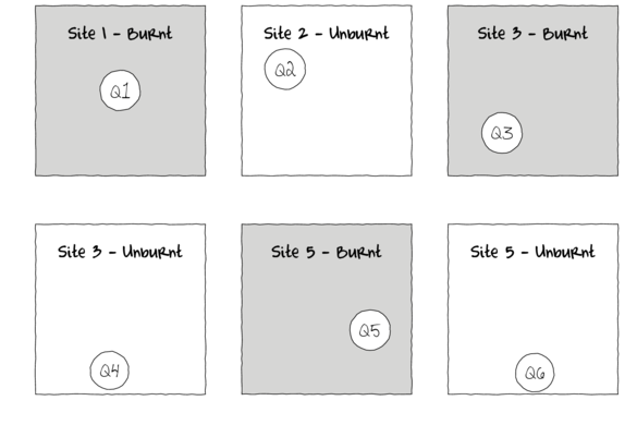
In the depiction of a single factor ANOVA below, a single quadrat has been randomly placed in each of the six Sites. If the conditions within each site were very heterogeneous, then the exact location of the quadrat in the site is likely to be very important.
As a result, the amount of variation within the main treatment effect (unexplained variability or noise) remains high thereby potentially masking any detectable effects (the signal) due to the measured treatments. Although this problem can be addressed by increased replication (having more sites of each treatment type), this is not always practical or possible.
For example, if we were investigating the impacts of fuel reduction burning across a highly heterogeneous landscape, our ability to replicate adequately might be limited by the number of burn sites available.
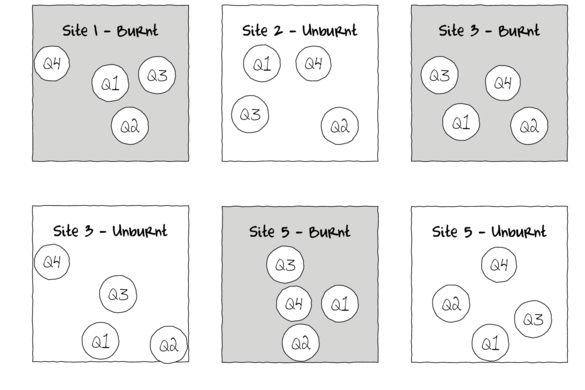
Alternatively, sub-replicates within each of the sampling units (e.g.~sites) can be collected (and averaged) so as to provided better representatives for each of the units (see the figure below) and ultimately reduce the unexplained variability of the test of treatments.
In essence, the sub-replicates are the replicates of an additional nested factor whose levels are nested within the main treatment factor. A nested factor refers to a factor whose levels are unique within each level of the factor it is nested within and each level is only represented once.
For example, the fuel reduction burn study design could consist of three burnt sites and three un-burnt (control) sites each containing four quadrats (replicates of site and sub-replicates of the burn treatment). Each site represents a unique level of a random factor (any given site cannot be both burnt and un-burnt) that is nested within the fire treatment (burned or not).
A nested design can be thought of as a hierarchical arrangement of factors (hence the alternative name hierarchical designs) whereby a treatment is progressively sub-replicated.
As an additional example, imagine an experiment designed to comparing the leaf toughness of a number of tree species. Working down the hierarchy, five individual trees were randomly selected within (nested within) each species, three branches were randomly selected within each tree, two leaves were randomly selected within each branch and the force required to shear the leaf material in half (transversely) was measured in four random locations along the leaf. Clearly any given leaf can only be from a single branch, tree and species.
Each level of sub-replication is introduced to further reduce the amount of unexplained variation and thereby increasing the power of the test for the main treatment effect. Additionally, it is possible to investigate which scale has the greatest (or least, etc) degree of variability - the level of the species, individual tree, branch, leaf, leaf region etc.
Nested factors are typically random factors, of which the levels are randomly selected to represent all possible levels (e.g.~sites). When the main treatment effect (often referred to as Factor A) is a fixed factor, such designs are referred to as a mixed model nested ANOVA, whereas when Factor A is random, the design is referred to as a Model II nested ANOVA.
Fixed nested factors are also possible. For example, specific dates (corresponding to particular times during a season) could be nested within season. When all factors are fixed, the design is referred to as a Model I mixed model.
Fully nested designs (the topic of this chapter) differ from other multi-factor designs in that all factors within (below) the main treatment factor are nested and thus interactions are un-replicated and cannot be tested. Indeed, interaction effects (interaction between Factor A and site) are assumed to be zero.
Linear models
The linear models for two and three factor nested design are:
$$y_{ijk}=\mu+\alpha_i + \beta_{j(i)} + \varepsilon_{ijk}$$
$$y_{ijkl}=\mu+\alpha_i + \beta_{j(i)} + \gamma_{k(j(i))} + \varepsilon_{ijkl}$$
where $\mu$ is the overall mean, $\alpha$ is the effect of Factor A, $\beta$ is the effect of Factor B, $\gamma$ is the effect of Factor C and $\varepsilon$ is the random unexplained or residual component.
Null hypotheses
Separate null hypotheses are associated with each of the factors, however, nested factors are typically only added to absorb some of the unexplained variability and thus, specific hypotheses tests associated with nested factors are of lesser biological importance. Hence, rather than estimate the effects of random effects, we instead estimate how much variability they contribute.
Factor A - the main treatment effect
Fixed
H$_0(A)$: $\mu_1=\mu_2=...=\mu_i=\mu$ (the population group means are all equal)
The mean of population 1 is equal to that of population 2 and so on, and thus all population means are equal to an overall mean.
If the effect of the $i^{th}$ group is the difference between the $i^{th}$ group mean and the overall mean ($\alpha_i = \mu_i - \mu$) then the H$_0$ can alternatively be written as:
H$_0(A)$: $\alpha_1 = \alpha_2 = ... = \alpha_i = 0$ (the effect of each group equals zero)
If one or more of the $\alpha_i$ are different from zero (the response mean for this treatment differs from the overall response mean), the null hypothesis is not true indicating that the treatment does affect the response variable.
Random
H$_0(A)$: $\sigma_\alpha^2=0$ (population variance equals zero)
There is no added variance due to all possible levels of A.
Factor B - the nested factor
Random (typical case)
H$_0(B)$: $\sigma_\beta^2=0$ (population variance equals zero)
There is no added variance due to all possible levels of B within the (set or all possible) levels of A.
Fixed
H$_0(B)$: $\mu_{1(1)}=\mu_{2(1)}=...=\mu_{j(i)}=\mu$ (the population group means of B (within A) are all equal)
H$_0(B)$: $\beta_{1(1)} = \beta_{2(1)}= ... = \beta_{j(i)} = 0$ (the effect of each chosen B group equals zero)
The null hypotheses associated with additional factors, are treated similarly to Factor B above.
Analysis of variance
Analysis of variance sequentially partitions the total variability in the response variable into components explained by each of the factors (starting with the factors lowest down in the hierarchy - the most deeply nested) and the components unexplained by each factor. Explained variability is calculated by subtracting the amount unexplained by the factor from the amount unexplained by a reduced model that does not contain the factor.
When the null hypothesis for a factor is true (no effect or added variability), the ratio of explained and unexplained components for that factor (F-ratio) should follow a theoretical F-distribution with an expected value less than 1. The appropriate unexplained residuals and therefore the appropriate F-ratios for each factor differ according to the different null hypotheses associated with different combinations of fixed and random factors in a nested linear model (see Table below).
| A fixed/random, B random | A fixed/random, B fixed | ||||||
|---|---|---|---|---|---|---|---|
| Factor | d.f | MS | F-ratio | Var. comp. | F-ratio | Var.comp. | |
| A | $a-1$ | $MS_A$ | $\frac{MS_A}{MS_{B^{\prime}(A)}}$ | $\frac{MS_A - MS_{B^{\prime}(A)}}{nb}$ | $\frac{MS_A}{MS_{Resid}}$ | $\frac{MS_A - MS_{Resid}}{nb}$ | |
| B$^{\prime}$(A) | $(b-1)a$ | $MS_{B^{\prime}(A)}$ | $\frac{MS_{B^{\prime}(A)}}{MS_{Resid}}$ | $\frac{MS_{B^{\prime}(A)} - MS_{Resid}}{n}$ | $\frac{MS_{B^{\prime}(A)}}{MS_{Resid}}$ | $\frac{MS_{B^{\prime}(A)} - MS_{Resid}}{n}$ | |
| Residual (=$N^{\prime}(B^{\prime}(A))$) | $(n-1)ba$ | $MS_{Resid}$ | |||||
| A fixed/random, B random | |||||||
summary(aov(y~A+Error(B), data)) library(nlme) VarCorr(lme(y~A,random=1|B, data)) |
|||||||
| Unbalanced |
library(nlme) anova(lme(y~A,random=1|B, data), type='marginal') |
||||||
| A fixed/random, B fixed | |||||||
summary(aov(y~A+B, data)) |
|||||||
| Unbalanced |
contrasts(data$B) <- contr.sum library(car) Anova(aov(y~A/B, data), type='III') |
||||||
Variance components
As previously alluded to, it can often be useful to determine the relative contribution (to explaining the unexplained variability) of each of the factors as this provides insights into the variability at each different scales.
These contributions are known as Variance components and are estimates of the added variances due to each of the factors. For consistency with leading texts on this topic, I have included estimated variance components for various balanced nested ANOVA designs in the above table. However, variance components based on a modified version of the maximum likelihood iterative model fitting procedure (REML) is generally recommended as this accommodates both balanced and unbalanced designs.
While there are no numerical differences in the calculations of variance components for fixed and random factors, fixed factors are interpreted very differently and arguably have little biological meaning (other to infer relative contribution). For fixed factors, variance components estimate the variance between the means of the specific populations that are represented by the selected levels of the factor and therefore represent somewhat arbitrary and artificial populations. For random factors, variance components estimate the variance between means of all possible populations that could have been selected and thus represents the true population variance.
Assumptions
An F-distribution represents the relative frequencies of all the possible F-ratio's when a given null hypothesis is true and certain assumptions about the residuals (denominator in the F-ratio calculation) hold.
Consequently, it is also important that diagnostics associated with a particular hypothesis test reflect the denominator for the appropriate F-ratio. For example, when testing the null hypothesis that there is no effect of Factor A (H$_0(A): \alpha_i=0$) in a mixed nested ANOVA, the means of each level of Factor B are used as the replicates of Factor A.
As with single factor anova, hypothesis testing for nested ANOVA assumes the residuals are:
- normally distributed. Factors higher up in the hierarchy of a nested model are based on means (or means of means) of lower factors and thus the Central Limit Theory would predict that normality will usually be satisfied for the higher level factors. Nevertheless, boxplots using the appropriate scale of replication should be used to explore normality. Scale transformations are often useful.
- equally varied. Boxplots and plots of means against variance (using the appropriate scale of replication) should be used to explore the spread of values. Residual plots should reveal no patterns (see Figure~\ref{fig:correlationRegression.residualPlotDiagnostics}). Scale transformations are often useful.
- independent of one another - this requires special consideration so as to ensure that the scale at which sub-replicates are measured is still great enough to enable observations to be independent.
Pooling denominator terms
Designs that incorporate fixed and random factors (either nested or factorial), involve F-ratio calculations in which the denominators are themselves random factors other than the overall residuals. Many statisticians argue that when such denominators are themselves not statistically significant (at the 0.25 level), there are substantial power benefits from pooling together successive non-significant denominator terms. Thus an F-ratio for a particular factor might be recalculated after pooling together its original denominator with its denominators denominator and so on.
The conservative 0.25 is used instead of the usual 0.05 to reduce further the likelihood of Type II errors (falsely concluding an effect is non-significant - that might result from insufficient power).
Unbalanced nested designs
For a simple completely balanced nested ANOVA, it is possible to pool together (calculate their mean) each of the sub-replicates within each nest (=site) and then perform single factor ANOVA on those aggregates. Indeed, for a balanced design, the estimates and hypothesis for Factor A will be identical to that produced via nested ANOVA.
However, if there are an unequal number of sub-replicates within each nest, then the single factor ANOVA will be less powerful that a proper nested ANOVA.
Unbalanced designs are those designs in which sample (subsample) sizes for each level of one or more factors differ. These situations are relatively common in biological research, however such imbalance has some important implications for nested designs.
- Firstly, hypothesis tests are more robust to the assumptions of normality and equal variance when the design is balanced.
- Secondly (and arguably, more importantly), the model contrasts are not orthogonal (independent) and the sums of squares component attributed to each of the model terms cannot be calculated by simple additive partitioning of the total sums of squares.
The severity of this issue depends on which scale of the sub-sampling hierarchy the unbalance(s) occurs as well whether the unbalance occurs in the replication of a fixed or random factor. For example, whilst unequal levels of the first nesting factor (e.g. unequal number of burn vs un-burnt sites) has no effect on F-ratio construction or hypothesis testing for the top level factor (irrespective of whether either of the factors are fixed or random), unequal sub-sampling (replication) at the level of a random (but not fixed) nesting factor will impact on the ability to construct F-ratios and variance components of all terms above it in the hierarchy.
There are a number of alternative ways of dealing with unbalanced nested designs. All alternatives assume that the imbalance is not a direct result of the treatments themselves. Such outcomes are more appropriately analysed by modelling the counts of surviving observations via frequency analysis.
- Split the analysis up into separate smaller simple ANOVA's each using the means of the nesting factor to reflect the appropriate scale of replication. As the resulting sums of squares components are thereby based on an aggregated dataset the analyses then inherit the procedures and requirements of single ANOVA.
- Adopt mixed-modelling techniques (see below).
Linear mixed effects models
Although the term `mixed-effects' can be used to refer to any design that incorporates both fixed and random predictors, its use is more commonly restricted to designs in which factors are nested or grouped within other factors. Typical examples include nested, longitudinal (measurements repeated over time) data, repeated measures and blocking designs.
Furthermore, rather than basing parameter estimations on observed and expected mean squares or error strata (as outline above), mixed-effects models estimate parameters via maximum likelihood (ML) or residual maximum likelihood (REML). In so doing, mixed-effects models more appropriately handle estimation of parameters, effects and variance components of unbalanced designs (particularly for random effects).
Resulting fitted (or expected) values of each level of a factor (for example, the expected population site means) are referred to as Best Linear Unbiased Predictors (BLUP's). As an acknowledgement that most estimated site means will be more extreme than the underlying true population means they estimate (based on the principle that smaller sample sizes result in greater chances of more extreme observations and that nested sub-replicates are also likely to be highly intercorrelated), BLUP's are less spread from the overall mean than are simple site means. In addition, mixed-effects models naturally model the 'within-block' correlation structure that complicates many longitudinal designs.
Whilst the basic concepts of mixed-effects models have been around for a long time, recent computing advances and adoptions have greatly boosted the popularity of these procedures.
Linear mixed effects models are currently at the forefront of statistical development, and as such, are very much a work in progress - both in theory and in practice. Recent developments have seen a further shift away from the traditional practices associated with degrees of freedom, probability distribution and p-value calculations.
The traditional approach to inference testing is to compare the fit of an alternative (full) model to a null (reduced) model (via an F-ratio). When assumptions of normality and homogeneity of variance apply, the degrees of freedom are easily computed and the F-ratio has an exact F-distribution to which it can be compared.
However, this approach introduces two additional problematic assumptions when estimating fixed effects in a mixed effects model. Firstly, when estimating the effects of one factor, the parameter estimates associated with other factor(s) are assumed to be the true values of those parameters (not estimates). Whilst this assumption is reasonable when all factors are fixed, as random factors are selected such that they represent one possible set of levels drawn from an entire population of possible levels for the random factor, it is unlikely that the associated parameter estimates accurately reflect the true values. Consequently, there is not necessarily an appropriate F-distribution.
Furthermore, determining the appropriate degrees of freedom (nominally, the number of independent observations on which estimates are based) for models that incorporate a hierarchical structure is only possible under very specific circumstances (such as completely balanced designs).
Degrees of freedom is a somewhat arbitrary defined concept used primarily to select a theoretical probability distribution on which a statistic can be compared. Arguably, however, it is a concept that is overly simplistic for complex hierarchical designs.
Most statistical applications continue to provide the `approximate' solutions (as did earlier versions within R). However, R linear mixed effects development leaders argue strenuously that given the above shortcomings, such approximations are variably inappropriate and are thus omitted.
MCMC sampling
Markov chain Monte Carlo (MCMC) sampling methods provide a Bayesian-like alternative for inference testing. Markov chains use the mixed model parameter estimates to generate posterior probability distributions of each parameter from which Monte Carlo sampling methods draw a large set of parameter samples.
These parameter samples can then be used to calculate highest posterior density (HPD) intervals (also known as Bayesian credible intervals). Such intervals indicate the interval in which there is a specified probability (typically 95%) that the true population parameter lies. Furthermore, whilst technically against the spirit of the Bayesian philosophy, it is also possible to generate P values on which to base inferences.
Nested ANOVA in R
| Routine | lme | lmer | glmmTMB |
|---|---|---|---|
| fit model | nlme::lme(y~A, random=~1|B, data) | lme4::lmer(y~x+(1|B), data) | glmmTMB::glmmTMB(y~x+(1|B), data) |
| raw residuals | residuals(mod) | residuals(mod) | residuals(mod) |
| standardized residuals | residuals(mod, type='pearson') | residuals(mod, type='pearson') | residuals(mod, type='pearson') |
| normalized residuals | rstandard(mod) | residuals(mod, type='pearson', scaled=TRUE) |
Scenario and Data
Imagine we has designed an experiment in which we intend to measure a response ($y$) to one of treatments (three levels; 'a1', 'a2' and 'a3'). The treatments occur at a spatial scale (over an area) that far exceeds the logistical scale of sampling units (it would take too long to sample at the scale at which the treatments were applied). The treatments occurred at the scale of hectares whereas it was only feasible to sample $y$ using 1m quadrats.
Given that the treatments were naturally occurring (such as soil type), it was not possible to have more than five sites of each treatment type, yet prior experience suggested that the sites in which you intended to sample were very uneven and patchy with respect to $y$.
In an attempt to account for this inter-site variability (and thus maximize the power of the test for the effect of treatment, you decided to employ a nested design in which 10 quadrats were randomly located within each of the five replicate sites per three treatments. As this section is mainly about the generation of artificial data (and not specifically about what to do with the data), understanding the actual details are optional and can be safely skipped. Consequently, I have folded (toggled) this section away.
- the number of treatments = 3
- the number of sites per treatment = 5
- the total number of sites = 15
- the sample size per treatment= 5
- the number of quadrats per site = 10
- the mean of the treatments = 40, 70 and 80 respectively
- the variability (standard deviation) between sites of the same treatment = 12
- the variability (standard deviation) between quadrats within sites = 5
set.seed(1)
nTreat <- 3
nSites <- 15
nSitesPerTreat <- nSites/nTreat
nQuads <- 10
site.sigma <- 12
sigma <- 5
n <- nSites * nQuads
sites <- gl(n = nSites, k = nQuads, lab = paste0("S", 1:nSites))
A <- gl(nTreat, nSitesPerTreat * nQuads, n, labels = c("a1", "a2", "a3"))
a.means <- c(40, 70, 80)
## the site means (treatment effects) are drawn from normal distributions with means of 40, 70 and 80
## and standard deviations of 12
A.effects <- rnorm(nSites, rep(a.means, each = nSitesPerTreat), site.sigma)
Xmat <- model.matrix(~sites - 1)
lin.pred <- Xmat %*% c(A.effects)
## the quadrat observations (within sites) are drawn from normal distributions with means according to
## the site means and standard deviations of 5
y <- rnorm(n, lin.pred, sigma)
data.nest <- data.frame(y = y, A = A, Sites = sites, Quads = 1:length(y))
head(data.nest)  #print out the first six rows of the data set
         y  A Sites Quads
1 32.25789 a1    S1     1
2 32.40160 a1    S1     2
3 37.20174 a1    S1     3
4 36.58866 a1    S1     4
5 35.45206 a1    S1     5
6 37.07744 a1    S1     6
library(ggplot2)
ggplot(data.nest, aes(y = y, x = 1)) + geom_boxplot() + facet_grid(. ~ Sites)

Exploratory data analysis
Normality and homogeneity of variance
Recall that in the nested design the observations are collected at a sub-replicate rather than the replicate level. That is, the actual replicates of the main treatment effect are the blocks not the quadrats. Therefore, when assessing assumptions pertaining to the residuals, it is necessary to first aggregate the observations to the blocks (=sites) - use the average of quadrats within each block as the replicates for the blocks.
library(tidyverse)
# calculate the site means
data.nest.agg = data.nest %>% group_by(A, Sites) %>% summarize(y = mean(y))
data.nest.agg
# A tibble: 15 x 3
# Groups:   A [?]
   A     Sites     y
   <fct> <fct> <dbl>
 1 a1    S1     33.8
 2 a1    S2     41.4
 3 a1    S3     30.5
 4 a1    S4     60.0
 5 a1    S5     45.6
 6 a2    S6     60.3
 7 a2    S7     75.3
 8 a2    S8     81.8
 9 a2    S9     74.4
10 a2    S10    68.8
11 a3    S11    98.0
12 a3    S12    83.9
13 a3    S13    69.0
14 a3    S14    51.5
15 a3    S15    94.1
boxplot(y ~ A, data.nest.agg)

ggplot(data.nest.agg, aes(y = y, x = A)) + geom_boxplot()

Conclusions: no obvious violations of non-normality or homogeneity of variance. Note that assessing normality can be a little difficult from such small numbers of replicates (5 sites per treatment).
Design balance
replications(y ~ A + Error(Sites), data.nest)
 A
50
# OR
replications(y ~ A + Sites, data.nest)
    A Sites
   50    10
Conclusions: the design is balanced and therefore type I (sequential) sums of squares are appropriate (if required).
Model fitting or statistical analysis
There are numerous ways of fitting a nested ANOVA in R.
Linear mixed effects modelling via the lme() function. This method is one of the original implementations in which separate variance-covariance matrices are incorporated into a interactive sequence of (generalized least squares) and maximum likelihood (actually REML) estimates of 'fixed' and 'random effects'.
Rather than fit just a single, simple random intercepts model, it is common to fit other related alternative models and explore which model fits the data best. For example, we could also fit a random intercepts and slope model. We could also explore other variance-covariance structures (autocorrelation or heterogeneity).
library(nlme)
# random intercept
data.nest.lme <- lme(y ~ A, random = ~1 | Sites, data.nest, method = "REML")
# random intercept/slope
data.nest.lme1 <- lme(y ~ A, random = ~A | Sites, data.nest, method = "REML")
anova(data.nest.lme, data.nest.lme1)
               Model df      AIC      BIC    logLik   Test  L.Ratio p-value
data.nest.lme      1  5 927.7266 942.6788 -458.8633
data.nest.lme1     2 10 934.7325 964.6369 -457.3663 1 vs 2 2.994092  0.7009
More modern linear mixed effects modelling via the lmer() function. In contrast to the lme() function, the lmer() function supports are more complex combination of random effects (such as crossed random effects). However, unfortunately, it does not yet (and probably never will) have a mechanism to support specifying alternative covariance structures needed to accommodate spatial and temporal autocorrelation
library(lme4)
data.nest.lmer <- lmer(y ~ A + (1 | Sites), data.nest, REML = TRUE)  #random intercept
data.nest.lmer1 <- lmer(y ~ A + (A | Sites), data.nest, REML = TRUE)  #random intercept/slope
anova(data.nest.lmer, data.nest.lmer1)
Data: data.nest
Models:
data.nest.lmer: y ~ A + (1 | Sites)
data.nest.lmer1: y ~ A + (A | Sites)
                Df    AIC    BIC  logLik deviance  Chisq Chi Df Pr(>Chisq)
data.nest.lmer   5 943.78 958.83 -466.89   933.78
data.nest.lmer1 10 950.04 980.15 -465.02   930.04 3.7426      5      0.587
Mixed effects models can also be fit using the Template Model Builder automatic differentiation engine via the glmmTMB() function from a package with the same name. glmmTMB is able to fit similar models to lmer, yet can also incorporate more complex features such as zero inflation and temporal autocorrelation. Random effects are assumed to be Gaussian on the scale of the linear predictor and are integrated out via Laplace approximation. On the downsides, REML is not available for this technique yet and nor is Gauss-Hermite quadrature (which can be useful when dealing with small sample sizes and non-gaussian errors.
library(glmmTMB)
data.nest.glmmTMB <- glmmTMB(y ~ A + (1 | Sites), data.nest)  #random intercept
data.nest.glmmTMB1 <- glmmTMB(y ~ A + (A | Sites), data.nest)  #random intercept/slope
anova(data.nest.glmmTMB, data.nest.glmmTMB1)
Data: data.nest
Models:
data.nest.glmmTMB: y ~ A + (1 | Sites), zi=~0, disp=~1
data.nest.glmmTMB1: y ~ A + (A | Sites), zi=~0, disp=~1
                   Df    AIC    BIC  logLik deviance Chisq Chi Df Pr(>Chisq)
data.nest.glmmTMB   5 943.78 958.83 -466.89   933.78
data.nest.glmmTMB1 10                                           5
Traditional OLS with multiple error strata using the aov() function. The aov() function is actually a wrapper for a specialized lm() call that defines multiple residual terms and thus adds some properties and class attributes to the fitted model that modify the output. This option is illustrated purely as a link to the past, it is no longer considered as robust or flexible as more modern techniques.
data.nest.aov <- aov(y ~ A + Error(Sites), data.nest)
Model evaluation
Residuals
As always, exploring the residuals can reveal issues of heteroscadacity, non-linearity and potential issues with autocorrelation. Note for lme() and lmer() residual plots use standardized (normalized) residuals rather than raw residuals as the former reflect changes to the variance-covariance matrix whereas the later do not.
The following function will be used for the production of some of the qqnormal plots.
qq.line = function(x) {
    # following four lines from base R's qqline()
    y <- quantile(x[!is.na(x)], c(0.25, 0.75))
    x <- qnorm(c(0.25, 0.75))
    slope <- diff(y)/diff(x)
    int <- y[1L] - slope * x[1L]
    return(c(int = int, slope = slope))
}
plot(data.nest.lme)

qqnorm(resid(data.nest.lme))
qqline(resid(data.nest.lme))

library(sjPlot)
plot_grid(plot_model(data.nest.lme, type = "diag"))

plot(data.nest.lmer)

plot(fitted(data.nest.lmer), residuals(data.nest.lmer, type = "pearson",
    scaled = TRUE))

ggplot(fortify(data.nest.lmer), aes(y = .scresid, x = .fitted)) +
    geom_point()

QQline = qq.line(fortify(data.nest.lmer)$.scresid)
ggplot(fortify(data.nest.lmer), aes(sample = .scresid)) + stat_qq() +
    geom_abline(intercept = QQline[1], slope = QQline[2])

qqnorm(resid(data.nest.lmer))
qqline(resid(data.nest.lmer))

library(sjPlot)
plot_grid(plot_model(data.nest.lmer, type = "diag"))

ggplot(data = NULL, aes(y = resid(data.nest.glmmTMB, type = "pearson"),
    x = fitted(data.nest.glmmTMB))) + geom_point()

QQline = qq.line(resid(data.nest.glmmTMB, type = "pearson"))
ggplot(data = NULL, aes(sample = resid(data.nest.glmmTMB, type = "pearson"))) +
    stat_qq() + geom_abline(intercept = QQline[1], slope = QQline[2])

library(sjPlot)
plot_grid(plot_model(data.nest.glmmTMB, type = "diag"))  #not working yet - bug
Error in UseMethod("rstudent"): no applicable method for 'rstudent' applied to an object of class "glmmTMB"
par(mfrow = c(2, 2))
plot(lm(data.nest.aov))

Exploring model parameters
If there was any evidence that the assumptions had been violated, then we would need to reconsider the model and start the process again. In this case, there is no evidence that the test will be unreliable so we can proceed to explore the test statistics. As I had elected to illustrate multiple techniques for analysing this nested design, I will also deal with the summaries etc separately.
Partial effects plots
It is often useful to visualize partial effects plots while exploring the parameter estimates. Having a graphical representation of the partial effects typically makes it a lot easier to interpret the parameter estimates and inferences.
library(effects)
plot(allEffects(data.nest.lme))

library(sjPlot)
plot_model(data.nest.lme, type = "eff", terms = "A")

library(effects)
plot(allEffects(data.nest.lmer))

library(sjPlot)
plot_model(data.nest.lmer, type = "eff", terms = "A")

library(ggeffects)
# observation level effects averaged across margins
p = ggaverage(data.nest.glmmTMB, terms = "A")
p = cbind(p, A = levels(data.nest$A))
ggplot(p, aes(y = predicted, x = A)) + geom_pointrange(aes(ymin = conf.low,
    ymax = conf.high))

# marginal effects
p = ggpredict(data.nest.glmmTMB, terms = "A")
p = cbind(p, A = levels(data.nest$A))
ggplot(p, aes(y = predicted, x = A)) + geom_pointrange(aes(ymin = conf.low,
    ymax = conf.high))

summary(data.nest.lme)
Linear mixed-effects model fit by REML
 Data: data.nest
       AIC      BIC    logLik
  927.7266 942.6788 -458.8633

Random effects:
 Formula: ~1 | Sites
        (Intercept) Residual
StdDev:     13.6582 4.372252

Fixed effects: y ~ A
               Value Std.Error  DF  t-value p-value
(Intercept) 42.27936  6.139350 135 6.886618  0.0000
Aa2         29.84692  8.682352  12 3.437654  0.0049
Aa3         37.02026  8.682352  12 4.263851  0.0011
 Correlation:
    (Intr) Aa2
Aa2 -0.707
Aa3 -0.707  0.500

Standardized Within-Group Residuals:
         Min           Q1          Med           Q3          Max
-2.603787242 -0.572951701  0.004953998  0.620914933  2.765601716

Number of Observations: 150
Number of Groups: 15
intervals(data.nest.lme)
Approximate 95% confidence intervals

 Fixed effects:
               lower     est.    upper
(Intercept) 30.13761 42.27936 54.42110
Aa2         10.92970 29.84692 48.76414
Aa3         18.10304 37.02026 55.93748
attr(,"label")
[1] "Fixed effects:"

 Random Effects:
  Level: Sites
                   lower    est.    upper
sd((Intercept)) 9.117188 13.6582 20.46096

 Within-group standard error:
   lower     est.    upper
3.880632 4.372252 4.926153
anova(data.nest.lme)
            numDF denDF  F-value p-value
(Intercept)     1   135 331.8308  <.0001
A               2    12  10.2268  0.0026
library(broom)
tidy(data.nest.lme, effects = "fixed")
         term estimate std.error statistic      p.value
1 (Intercept) 42.27936  6.139350  6.886618 1.968597e-10
2         Aa2 29.84692  8.682352  3.437654 4.915711e-03
3         Aa3 37.02026  8.682352  4.263851 1.099991e-03
glance(data.nest.lme)
     sigma    logLik      AIC      BIC deviance
1 4.372252 -458.8633 927.7266 942.6788       NA
summary(data.nest.lmer)
Linear mixed model fit by REML ['lmerMod']
Formula: y ~ A + (1 | Sites)
   Data: data.nest

REML criterion at convergence: 917.7

Scaled residuals:
     Min       1Q   Median       3Q      Max
-2.60379 -0.57295  0.00495  0.62091  2.76560

Random effects:
 Groups   Name        Variance Std.Dev.
 Sites    (Intercept) 186.55   13.658
 Residual              19.12    4.372
Number of obs: 150, groups:  Sites, 15

Fixed effects:
            Estimate Std. Error t value
(Intercept)   42.279      6.139   6.887
Aa2           29.847      8.682   3.438
Aa3           37.020      8.682   4.264

Correlation of Fixed Effects:
    (Intr) Aa2
Aa2 -0.707
Aa3 -0.707  0.500
confint(data.nest.lmer)
                2.5 %    97.5 %
.sig01       8.810146 18.378060
.sigma       3.898371  4.950531
(Intercept) 30.789517 53.769198
Aa2         13.597836 46.096012
Aa3         20.771169 53.269345
anova(data.nest.lmer)
Analysis of Variance Table
  Df Sum Sq Mean Sq F value
A  2    391   195.5  10.227
library(broom)
tidy(data.nest.lmer, effects = "fixed")
         term estimate std.error statistic
1 (Intercept) 42.27936  6.139350  6.886618
2         Aa2 29.84692  8.682352  3.437654
3         Aa3 37.02026  8.682352  4.263851
glance(data.nest.lmer)
     sigma    logLik      AIC      BIC deviance df.residual
1 4.372252 -458.8633 927.7266 942.7798 934.0982         145
As a result of disagreement and discontent concerning the appropriate residual degrees of freedom, lmer() does not provide p-values in summary or anova tables. For hypothesis testing, the following options exist:
- Confidence intervals on the estimated parameters.
confint(data.nest.lmer)
                2.5 %    97.5 %
.sig01       8.810146 18.378060
.sigma       3.898371  4.950531
(Intercept) 30.789517 53.769198
Aa2         13.597836 46.096012
Aa3         20.771169 53.269345
- Likelihood Ratio Test (LRT). Note, as this is contrasting a fixed component, the models need to be fitted with ML rather than REML.
mod1 = update(data.nest.lmer, REML = FALSE)
mod2 = update(data.nest.lmer, ~. - A, REML = FALSE)
anova(mod1, mod2)
Data: data.nest Models: mod2: y ~ (1 | Sites) mod1: y ~ A + (1 | Sites) Df AIC BIC logLik deviance Chisq Chi Df Pr(>Chisq) mod2 3 954.71 963.74 -474.35 948.71 mod1 5 943.78 958.83 -466.89 933.78 14.924 2 0.0005746 *** --- Signif. codes: 0 '***' 0.001 '**' 0.01 '*' 0.05 '.' 0.1 ' ' 1 - Adopt the Satterthwaite or Kenward-Roger methods to denominator degrees of freedom (as used in SAS). This approach requires the lmerTest
and pbkrtest packages and requires that they be loaded before fitting the model (update() will suffice).
Note just because these are the approaches adopted by SAS, this does not mean that they are 'correct'.
library(lmerTest)
data.nest.lmer <- update(data.nest.lmer)
summary(data.nest.lmer)
Linear mixed model fit by REML t-tests use Satterthwaite approximations to degrees of freedom [ lmerMod] Formula: y ~ A + (1 | Sites) Data: data.nest REML criterion at convergence: 917.7 Scaled residuals: Min 1Q Median 3Q Max -2.60379 -0.57295 0.00495 0.62091 2.76560 Random effects: Groups Name Variance Std.Dev. Sites (Intercept) 186.55 13.658 Residual 19.12 4.372 Number of obs: 150, groups: Sites, 15 Fixed effects: Estimate Std. Error df t value Pr(>|t|) (Intercept) 42.279 6.139 12.000 6.887 1.68e-05 *** Aa2 29.847 8.682 12.000 3.438 0.00492 ** Aa3 37.020 8.682 12.000 4.264 0.00110 ** --- Signif. codes: 0 '***' 0.001 '**' 0.01 '*' 0.05 '.' 0.1 ' ' 1 Correlation of Fixed Effects: (Intr) Aa2 Aa2 -0.707 Aa3 -0.707 0.500anova(data.nest.lmer) # Satterthwaite denominator df method
Analysis of Variance Table of type III  with  Satterthwaite
approximation for degrees of freedom
  Sum Sq Mean Sq NumDF DenDF F.value   Pr(>F)
A    391   195.5     2    12  10.227 0.002556 **
---
Signif. codes:  0 '***' 0.001 '**' 0.01 '*' 0.05 '.' 0.1 ' ' 1
anova(data.nest.lmer, ddf = "Kenward-Roger")
Analysis of Variance Table of type III  with  Kenward-Roger
approximation for degrees of freedom
  Sum Sq Mean Sq NumDF DenDF F.value   Pr(>F)
A    391   195.5     2    12  10.227 0.002556 **
---
Signif. codes:  0 '***' 0.001 '**' 0.01 '*' 0.05 '.' 0.1 ' ' 1
summary(data.nest.glmmTMB)
 Family: gaussian  ( identity )
Formula:          y ~ A + (1 | Sites)
Data: data.nest

     AIC      BIC   logLik deviance df.resid
   943.8    958.8   -466.9    933.8      145

Random effects:

Conditional model:
 Groups   Name        Variance Std.Dev.
 Sites    (Intercept) 148.85   12.201
 Residual              19.12    4.372
Number of obs: 150, groups:  Sites, 15

Dispersion estimate for gaussian family (sigma^2): 19.1

Conditional model:
            Estimate Std. Error z value Pr(>|z|)
(Intercept)   42.279      5.491   7.699 1.37e-14 ***
Aa2           29.847      7.766   3.843 0.000121 ***
Aa3           37.020      7.766   4.767 1.87e-06 ***
---
Signif. codes:  0 '***' 0.001 '**' 0.01 '*' 0.05 '.' 0.1 ' ' 1
confint(data.nest.glmmTMB)
                                   2.5 %   97.5 %  Estimate
cond.(Intercept)               31.516763 53.04188 42.279319
cond.Aa2                       14.626378 45.06748 29.846932
cond.Aa3                       21.799758 52.24086 37.020311
cond.Std.Dev.Sites.(Intercept)  8.491352 17.53016 12.200606
sigma                           3.880634  4.92615  4.372252
summary(data.nest.aov)
Error: Sites
          Df Sum Sq Mean Sq F value  Pr(>F)
A          2  38547   19273   10.23 0.00256 **
Residuals 12  22615    1885
---
Signif. codes:  0 '***' 0.001 '**' 0.01 '*' 0.05 '.' 0.1 ' ' 1

Error: Within
           Df Sum Sq Mean Sq F value Pr(>F)
Residuals 135   2581   19.12
- there is a significant effect of factor A
- more specifically, level a2 and a3 are both significantly higher than level a1
- sites accounted for a substantial amount of variability
- if we required to compare each group with each other group via multiple pairwise comparisons (whilst controlling for type I error rates), we might also conclude that there was no evidence that groups a2 and a3 differed from one another.
Variance components
VarCorr(data.nest.lme)
Sites = pdLogChol(1)
            Variance  StdDev
(Intercept) 186.54644 13.658200
Residual     19.11659  4.372252
VarCorr(data.nest.lmer)
 Groups   Name        Std.Dev.
 Sites    (Intercept) 13.6582
 Residual              4.3723
VarCorr(data.nest.glmmTMB)
Conditional model:
 Groups   Name        Std.Dev.
 Sites    (Intercept) 12.2006
 Residual              4.3723
$R^2$ approximations
Whilst $R^2$ is a popular goodness of fit metric in simple linear models, its use is rarely extended to (generalized) linear mixed effects models. The reasons for this include:
- there are numerous ways that $R^2$ could be defined for mixed effects models, some of which can result in values that are either difficult to interpret or illogical (for example negative $R^2$).
- perhaps as a consequence, software implementation is also largely lacking.
Nakagawa and Schielzeth (2013) discuss the issues associated with $R^2$ calculations and
suggest a series of simple calculations to yield sensible $R^2$ values from mixed effects models.
An $R^2$ value quantifies the proportion of variance explained by a model (or by terms in a model) - the higher the
value, the better the model (or term) fit.
Nakagawa and Schielzeth (2013) offered up two $R^2$ for mixed effects models:
- Marginal $R^2$ - the proportion of total variance explained by the fixed effects. $$ \text{Marginal}~R^2 = \frac{\sigma^2_f}{\sigma^2_f + \sum^z_l{\sigma^2_l} + \sigma^2_d + \sigma^2_e} $$ where $\sigma^2_f$ is the variance of the fitted values (i.e. $\sigma^2_f = var(\mathbf{X\beta})$) on the link scale, $\sum^z_l{\sigma^2_l}$ is the sum of the $z$ random effects (including the residuals) and $\sigma^2_d$ and $\sigma^2_e$ are additional variance components appropriate when using non-Gaussian distributions.
- Conditional $R^2$ - the proportion of the total variance collectively explained by the fixed and random factors $$ \text{Conditional}~R^2 = \frac{\sigma^2_f + \sum^z_l{\sigma^2_l}}{\sigma^2_f + \sum^z_l{\sigma^2_l} + \sigma^2_d + \sigma^2_e} $$
library(MuMIn)
r.squaredGLMM(data.nest.lme)
      R2m       R2c
0.5571090 0.9588328
library(sjstats)
r2(data.nest.lme)
    R-squared: 0.9595
Omega-squared: 0.9595
library(MuMIn)
r.squaredGLMM(data.nest.lmer)
      R2m       R2c
0.5571090 0.9588328
library(sjstats)
r2(data.nest.lmer)
    R-squared: 0.9595
Omega-squared: 0.9595
source(system.file("misc/rsqglmm.R", package = "glmmTMB"))
my_rsq(data.nest.glmmTMB)
$family
[1] "gaussian"

$link
[1] "identity"

$Marginal
[1] 0.6063237

$Conditional
[1] 0.9551963
The fixed effect of A (within Block) accounts for approximately 55.71% of the total variation in Y.
The random effect of Block accounts for approximately 40.17% of the total variation in Y and collectively,
the hierarchical level of Block (containing the fixed effect) explains approximately 95.88% of the total variation in Y.
Graphical summary
It is relatively trivial to produce a summary figure based on the raw data. Arguably a more satisfying figure would be one based on the modelled data.
library(effects)
data.nest.eff = as.data.frame(allEffects(data.nest.lme)[[1]])
# OR
data.nest.eff = as.data.frame(Effect("A", data.nest.lme))

ggplot(data.nest.eff, aes(y = fit, x = A)) + geom_pointrange(aes(ymin = lower,
    ymax = upper)) + scale_y_continuous("Y") + theme_classic()

newdata = data.frame(A = levels(data.nest$A))
Xmat = model.matrix(~A, data = newdata)
coefs = fixef(data.nest.lme)
fit = as.vector(coefs %*% t(Xmat))
se = sqrt(diag(Xmat %*% vcov(data.nest.lme) %*% t(Xmat)))
q = qt(0.975, df = nrow(data.nest.lme$data) - length(coefs) -
    2)
newdata = cbind(newdata, fit = fit, lower = fit - q * se, upper = fit +
    q * se)
ggplot(newdata, aes(y = fit, x = A)) + geom_pointrange(aes(ymin = lower,
    ymax = upper)) + scale_y_continuous("Y") + theme_classic()

library(effects)
data.nest.eff = as.data.frame(allEffects(data.nest.lmer)[[1]])
# OR
data.nest.eff = as.data.frame(Effect("A", data.nest.lmer))

ggplot(data.nest.eff, aes(y = fit, x = A)) + geom_pointrange(aes(ymin = lower,
    ymax = upper)) + scale_y_continuous("Y") + theme_classic()

newdata = data.frame(A = levels(data.nest$A))
Xmat = model.matrix(~A, data = newdata)
coefs = fixef(data.nest.lmer)
fit = as.vector(coefs %*% t(Xmat))
se = sqrt(diag(Xmat %*% vcov(data.nest.lmer) %*% t(Xmat)))
q = qt(0.975, df = df.residual(data.nest.lmer))
newdata = cbind(newdata, fit = fit, lower = fit - q * se, upper = fit +
    q * se)
ggplot(newdata, aes(y = fit, x = A)) + geom_pointrange(aes(ymin = lower,
    ymax = upper)) + scale_y_continuous("Y") + theme_classic()

newdata = data.frame(A = levels(data.nest$A))
newdata = predict(data.nest.glmmTMB, re.form = NA, newdata = newdata,
    interval = "confidence")
Error in predict.glmmTMB(data.nest.glmmTMB, re.form = NA, newdata = newdata, : re.form not yet implemented
ggplot(newdata, aes(y = fit, x = A)) + geom_pointrange(aes(ymin = lower,
    ymax = upper)) + scale_y_continuous("Y") + theme_classic()
Error in eval(expr, envir, enclos): object 'lower' not found

newdata = data.frame(A = levels(data.nest$A))
Xmat = model.matrix(~A, data = newdata)
coefs = fixef(data.nest.glmmTMB)[[1]]
fit = as.vector(coefs %*% t(Xmat))
se = sqrt(diag(Xmat %*% vcov(data.nest.glmmTMB)[[1]] %*% t(Xmat)))
q = qt(0.975, df = df.residual(data.nest.glmmTMB))
newdata = cbind(newdata, fit = fit, lower = fit - q * se, upper = fit +
    q * se)
ggplot(newdata, aes(y = fit, x = A)) + geom_pointrange(aes(ymin = lower,
    ymax = upper)) + scale_y_continuous("Y") + theme_classic()

Another data set and scenario
Lets now add an additional hierarchical layer - sampling units within the quadrats.
- the number of treatments = 3
- the number of sites per treatment = 5
- the total number of sites = 15
- the sample size per treatment= 5
- the number of quadrats per site = 5
- the number of pits per quadrat = 2
- the mean of the treatments = 40, 70 and 80 respectively
- the variability (standard deviation) between sites of the same treatment = 12
- the variability (standard deviation) between quadrats within sites = 10
- the variability (standard deviation) between quadrats within sites = 5
set.seed(1)
nTreat <- 3
nSites <- 15
nSitesPerTreat <- nSites/nTreat
nQuads <- 5
nPits <- 2
site.sigma <- 15
quad.sigma <- 10
sigma <- 5
n <- nSites * nQuads * nPits
sites <- gl(n = nSites, n/nSites, n, lab = paste0("Site", 1:nSites))
A <- gl(nTreat, n/nTreat, n, labels = c("a1", "a2", "a3"))
a.means <- c(40, 70, 80)

# A<-gl(nTreat,nSites/nTreat,nSites,labels=c('a1','a2','a3'))
A <- gl(nTreat, 1, nTreat, labels = c("a1", "a2", "a3"))
a.X <- model.matrix(~A, expand.grid(A))
a.eff <- as.vector(solve(a.X, a.means))
# a.X <- model.matrix(~A,
# expand.grid(A=gl(nTreat,nSites/nTreat,nSites,labels=c('a1','a2','a3'))))
site.means <- rnorm(nSites, a.X %*% a.eff, site.sigma)

SITES <- gl(nSites, 1, nSites, labels = paste0("S", 1:nSites))
sites.X <- model.matrix(~SITES - 1)
# sites.eff <- as.vector(solve(sites.X,site.means)) quad.means <-
# rnorm(nSites*nQuads,sites.X %*% sites.eff,quad.sigma)
quad.means <- rnorm(nSites * nQuads, sites.X %*% site.means, quad.sigma)

QUADS <- gl(nQuads, nSites, n, labels = paste0("Q", 1:nQuads))
quads.X <- model.matrix(~SITES * QUADS, expand.grid(SITES = SITES,
    QUADS = factor(1:nQuads)))
quads.eff <- as.vector(solve(quads.X, quad.means))
pit.means <- rnorm(n, quads.eff %*% t(quads.X), sigma)

PITS <- gl(nPits, nSites * nQuads, n, labels = paste0("P", 1:nPits))
data.nest1 <- data.frame(Pits = PITS, Quads = QUADS, Sites = rep(SITES,
    5), A = rep(A, 50), y = pit.means)
data.nest1 <- data.nest1[order(data.nest1$A, data.nest1$Sites, data.nest1$Quads),
    ]
head(data.nest1)  #print out the first six rows of the data set
    Pits Quads Sites  A        y
1     P1    Q1    S1 a1 27.44126
76    P2    Q1    S1 a1 41.18437
16    P1    Q2    S1 a1 53.02642
91    P2    Q2    S1 a1 38.03337
31    P1    Q3    S1 a1 20.99845
106   P2    Q3    S1 a1 18.28832
library(ggplot2)
ggplot(data.nest1, aes(y = y, x = 1)) + geom_boxplot(aes(fill = A)) +
    facet_grid(~Sites * Quads)

Exploratory data analysis
library(plyr)
# calculate the site means
data.nest1.agg <- ddply(data.nest1, ~A + Sites, function(x) {
    data.frame(y = mean(x$y))
})
data.nest1.agg
    A Sites        y
1  a1    S1 37.80088
2  a1    S4 63.91939
3  a1    S7 43.19601
4  a1   S10 44.63361
5  a1   S13 27.90133
6  a2    S2 74.88463
7  a2    S5 74.08441
8  a2    S8 86.03434
9  a2   S11 97.40098
10 a2   S14 37.61487
11 a3    S3 71.43908
12 a3    S6 69.10660
13 a3    S9 79.84349
14 a3   S12 86.70191
15 a3   S15 92.37056
boxplot(y ~ A, data.nest1.agg)

ggplot(data.nest1.agg, aes(y = y, x = A)) + geom_boxplot()

replications(y ~ A + Error(Sites/Quads), data.nest1)
 A
50
# OR
replications(y ~ A + Sites + Quads, data.nest1)
    A Sites Quads
   50    10    30
Conclusions: there are no immediately obvious issues with the data (notwithstanding the difficulties of exploring normality and homogeneity from small sample sizes) and the design is balanced and therefore type I (sequential) sums of squares are appropriate
Model fitting or statistical analysis
Linear mixed effects modelling via the lme() function. This method is one of the original implementations in which separate variance-covariance matrices are incorporated into a interactive sequence of (generalized least squares) and maximum likelihood (actually REML) estimates of 'fixed' and 'random effects'.
Rather than fit just a single, simple random intercepts model, it is common to fit other related alternative models and explore which model fits the data best. For example, we could also fit a random intercepts and slope model. We could also explore other variance-covariance structures (autocorrelation or heterogeneity).
library(nlme)
data.nest1.lme <- lme(y ~ A, random = ~1 | Sites/Quads, data.nest1, method = "REML")
More modern linear mixed effects modelling via the lmer() function. In contrast to the lme() function, the lmer() function supports are more complex combination of random effects (such as crossed random effects). However, unfortunately, it does not yet (and probably never will) have a mechanism to support specifying alternative covariance structures needed to accommodate spatial and temporal autocorrelation
library(lme4)
data.nest1.lmer <- lmer(y ~ A + (1 | Sites/Quads), data.nest1, REML = TRUE)  #random intercept
Mixed effects models can also be fit using the Template Model Builder automatic differentiation engine via the glmmTMB() function from a package with the same name. glmmTMB is able to fit similar models to lmer, yet can also incorporate more complex features such as zero inflation and temporal autocorrelation. Random effects are assumed to be Gaussian on the scale of the linear predictor and are integrated out via Laplace approximation. On the downsides, REML is not available for this technique yet and nor is Gauss-Hermite quadrature (which can be useful when dealing with small sample sizes and non-gaussian errors.
library(glmmTMB)
data.nest1.glmmTMB <- glmmTMB(y ~ A + (1 | Sites/Quads), data.nest1)  #random intercept
Traditional OLS with multiple error strata using the aov() function. The aov() function is actually a wrapper for a specialized lm() call that defines multiple residual terms and thus adds some properties and class attributes to the fitted model that modify the output. This option is illustrated purely as a link to the past, it is no longer considered as robust or flexible as more modern techniques.
data.nest1.aov <- aov(y ~ A + Error(Sites/Quads), data.nest1)
Model evaluation
Residuals
As always, exploring the residuals can reveal issues of heteroscadacity, non-linearity and potential issues with autocorrelation. Note for lme() and lmer() residual plots use standardized (normalized) residuals rather than raw residuals as the former reflect changes to the variance-covariance matrix whereas the later do not.
The following function will be used for the production of some of the qqnormal plots.
qq.line = function(x) {
    # following four lines from base R's qqline()
    y <- quantile(x[!is.na(x)], c(0.25, 0.75))
    x <- qnorm(c(0.25, 0.75))
    slope <- diff(y)/diff(x)
    int <- y[1L] - slope * x[1L]
    return(c(int = int, slope = slope))
}
plot(data.nest1.lme)

qqnorm(resid(data.nest1.lme))
qqline(resid(data.nest1.lme))

library(sjPlot)
plot_grid(plot_model(data.nest1.lme, type = "diag"))

plot(data.nest1.lmer)

plot(fitted(data.nest1.lmer), residuals(data.nest1.lmer, type = "pearson",
    scaled = TRUE))

ggplot(fortify(data.nest1.lmer), aes(y = .scresid, x = .fitted)) +
    geom_point()

QQline = qq.line(fortify(data.nest1.lmer)$.scresid)
ggplot(fortify(data.nest1.lmer), aes(sample = .scresid)) + stat_qq() +
    geom_abline(intercept = QQline[1], slope = QQline[2])

qqnorm(resid(data.nest1.lmer))
qqline(resid(data.nest1.lmer))

library(sjPlot)
plot_grid(plot_model(data.nest1.lmer, type = "diag"))

ggplot(data = NULL, aes(y = resid(data.nest1.glmmTMB, type = "pearson"),
    x = fitted(data.nest1.glmmTMB))) + geom_point()

QQline = qq.line(resid(data.nest1.glmmTMB, type = "pearson"))
ggplot(data = NULL, aes(sample = resid(data.nest1.glmmTMB, type = "pearson"))) +
    stat_qq() + geom_abline(intercept = QQline[1], slope = QQline[2])

library(sjPlot)
plot_grid(plot_model(data.nest1.glmmTMB, type = "diag"))  #not working yet - bug
Error in UseMethod("rstudent"): no applicable method for 'rstudent' applied to an object of class "glmmTMB"
par(mfrow = c(2, 2))
plot(lm(data.nest1.aov))

Exploring model parameters
If there was any evidence that the assumptions had been violated, then we would need to reconsider the model and start the process again. In this case, there is no evidence that the test will be unreliable so we can proceed to explore the test statistics. As I had elected to illustrate multiple techniques for analysing this nested design, I will also deal with the summaries etc separately.
Partial effects plots
It is often useful to visualize partial effects plots while exploring the parameter estimates. Having a graphical representation of the partial effects typically makes it a lot easier to interpret the parameter estimates and inferences.
library(effects)
plot(allEffects(data.nest1.lme))

library(sjPlot)
plot_model(data.nest1.lme, type = "eff", terms = "A")

library(effects)
plot(allEffects(data.nest1.lmer))

library(sjPlot)
plot_model(data.nest1.lmer, type = "eff", terms = "A")

library(ggeffects)
# observation level effects averaged across margins
p = ggaverage(data.nest1.glmmTMB, terms = "A")
p = cbind(p, A = levels(data.nest1$A))
ggplot(p, aes(y = predicted, x = A)) + geom_pointrange(aes(ymin = conf.low,
    ymax = conf.high))

# marginal effects
p = ggpredict(data.nest1.glmmTMB, terms = "A")
p = cbind(p, A = levels(data.nest1$A))
ggplot(p, aes(y = predicted, x = A)) + geom_pointrange(aes(ymin = conf.low,
    ymax = conf.high))

summary(data.nest1.lme)
Linear mixed-effects model fit by REML
 Data: data.nest1
       AIC      BIC    logLik
  1079.258 1097.201 -533.6292

Random effects:
 Formula: ~1 | Sites
        (Intercept)
StdDev:    15.59142

 Formula: ~1 | Quads %in% Sites
        (Intercept) Residual
StdDev:    8.003042 5.023277

Fixed effects: y ~ A
               Value Std.Error DF  t-value p-value
(Intercept) 43.49024  7.189234 75 6.049357  0.0000
Aa2         30.51360 10.167113 12 3.001206  0.0110
Aa3         36.40209 10.167113 12 3.580376  0.0038
 Correlation:
    (Intr) Aa2
Aa2 -0.707
Aa3 -0.707  0.500

Standardized Within-Group Residuals:
        Min          Q1         Med          Q3         Max
-2.00020166 -0.47356371 -0.02493572  0.41710101  1.96210317

Number of Observations: 150
Number of Groups:
           Sites Quads %in% Sites
              15               75
intervals(data.nest1.lme)
Approximate 95% confidence intervals

 Fixed effects:
                lower     est.    upper
(Intercept) 29.168554 43.49024 57.81193
Aa2          8.361367 30.51360 52.66584
Aa3         14.249850 36.40209 58.55432
attr(,"label")
[1] "Fixed effects:"

 Random Effects:
  Level: Sites
                   lower     est.    upper
sd((Intercept)) 10.18847 15.59142 23.85955
  Level: Quads
                   lower     est.    upper
sd((Intercept)) 6.445288 8.003042 9.937288

 Within-group standard error:
   lower     est.    upper
4.280419 5.023277 5.895056
anova(data.nest1.lme)
            numDF denDF   F-value p-value
(Intercept)     1    75 251.27426  <.0001
A               2    12   7.38726  0.0081
library(broom)
tidy(data.nest1.lme, effects = "fixed")
         term estimate std.error statistic      p.value
1 (Intercept) 43.49024  7.189234  6.049357 5.276461e-08
2         Aa2 30.51360 10.167113  3.001206 1.104191e-02
3         Aa3 36.40209 10.167113  3.580376 3.779659e-03
glance(data.nest1.lme)
     sigma    logLik      AIC      BIC deviance
1 5.023277 -533.6292 1079.258 1097.201       NA
summary(data.nest1.lmer)
Linear mixed model fit by REML t-tests use Satterthwaite approximations to degrees of freedom [
lmerMod]
Formula: y ~ A + (1 | Sites/Quads)
   Data: data.nest1

REML criterion at convergence: 1067.3

Scaled residuals:
     Min       1Q   Median       3Q      Max
-2.00020 -0.47356 -0.02494  0.41710  1.96211

Random effects:
 Groups      Name        Variance Std.Dev.
 Quads:Sites (Intercept)  64.05    8.003
 Sites       (Intercept) 243.09   15.591
 Residual                 25.23    5.023
Number of obs: 150, groups:  Quads:Sites, 75; Sites, 15

Fixed effects:
            Estimate Std. Error     df t value Pr(>|t|)
(Intercept)   43.490      7.189 12.000   6.049 5.76e-05 ***
Aa2           30.514     10.167 12.000   3.001  0.01104 *
Aa3           36.402     10.167 12.000   3.580  0.00378 **
---
Signif. codes:  0 '***' 0.001 '**' 0.01 '*' 0.05 '.' 0.1 ' ' 1

Correlation of Fixed Effects:
    (Intr) Aa2
Aa2 -0.707
Aa3 -0.707  0.500
confint(data.nest1.lmer)
                2.5 %    97.5 %
.sig01       6.447283  9.985982
.sig02       9.668233 21.224272
.sigma       4.315254  5.948431
(Intercept) 30.035564 56.944921
Aa2         11.485813 49.541391
Aa3         17.374297 55.429875
anova(data.nest1.lmer)
Analysis of Variance Table of type III  with  Satterthwaite
approximation for degrees of freedom
  Sum Sq Mean Sq NumDF DenDF F.value   Pr(>F)
A 372.81  186.41     2    12  7.3873 0.008105 **
---
Signif. codes:  0 '***' 0.001 '**' 0.01 '*' 0.05 '.' 0.1 ' ' 1
library(broom)
tidy(data.nest1.lmer, effects = "fixed")
         term estimate std.error statistic
1 (Intercept) 43.49024  7.189221  6.049368
2         Aa2 30.51360 10.167094  3.001212
3         Aa3 36.40209 10.167094  3.580383
glance(data.nest1.lmer)
     sigma    logLik      AIC      BIC deviance df.residual
1 5.023292 -533.6292 1079.258 1097.322 1067.258         144
As a result of disagreement and discontent concerning the appropriate residual degrees of freedom, lmer() does not provide p-values in summary or anova tables. For hypothesis testing, the following options exist:
- Confidence intervals on the estimated parameters.
confint(data.nest1.lmer)
                2.5 %    97.5 %
.sig01       6.447283  9.985982
.sig02       9.668233 21.224272
.sigma       4.315254  5.948431
(Intercept) 30.035564 56.944921
Aa2         11.485813 49.541391
Aa3         17.374297 55.429875
- Likelihood Ratio Test (LRT). Note, as this is contrasting a fixed component, the models need to be fitted with ML rather than REML.
mod1 = update(data.nest1.lmer, REML = FALSE)
mod2 = update(data.nest1.lmer, ~. - A, REML = FALSE)
anova(mod1, mod2)
Data: data.nest1 Models: mod2: y ~ (1 | Sites/Quads) mod1: y ~ A + (1 | Sites/Quads) Df AIC BIC logLik deviance Chisq Chi Df Pr(>Chisq) mod2 4 1104.3 1116.3 -548.15 1096.3 mod1 6 1096.3 1114.3 -542.13 1084.3 12.038 2 0.002432 ** --- Signif. codes: 0 '***' 0.001 '**' 0.01 '*' 0.05 '.' 0.1 ' ' 1 - Adopt the Satterthwaite or Kenward-Roger methods to denominator degrees of freedom (as used in SAS). This approach requires the lmerTest
and pbkrtest packages and requires that they be loaded before fitting the model (update() will suffice).
Note just because these are the approaches adopted by SAS, this does not mean that they are 'correct'.
library(lmerTest)
data.nest1.lmer <- update(data.nest1.lmer)
summary(data.nest1.lmer)
Linear mixed model fit by REML ['lmerMod'] Formula: y ~ A + (1 | Sites/Quads) Data: data.nest1 REML criterion at convergence: 1067.3 Scaled residuals: Min 1Q Median 3Q Max -2.00020 -0.47356 -0.02494 0.41710 1.96211 Random effects: Groups Name Variance Std.Dev. Quads:Sites (Intercept) 64.05 8.003 Sites (Intercept) 243.09 15.591 Residual 25.23 5.023 Number of obs: 150, groups: Quads:Sites, 75; Sites, 15 Fixed effects: Estimate Std. Error t value (Intercept) 43.490 7.189 6.049 Aa2 30.514 10.167 3.001 Aa3 36.402 10.167 3.580 Correlation of Fixed Effects: (Intr) Aa2 Aa2 -0.707 Aa3 -0.707 0.500anova(data.nest1.lmer) # Satterthwaite denominator df method
Analysis of Variance Table
  Df Sum Sq Mean Sq F value
A  2 372.81  186.41  7.3873
anova(data.nest1.lmer, ddf = "Kenward-Roger")
Analysis of Variance Table
  Df Sum Sq Mean Sq F value
A  2 372.81  186.41  7.3873
summary(data.nest1.glmmTMB)
 Family: gaussian  ( identity )
Formula:          y ~ A + (1 | Sites/Quads)
Data: data.nest1

     AIC      BIC   logLik deviance df.resid
  1096.3   1114.3   -542.1   1084.3      144

Random effects:

Conditional model:
 Groups      Name        Variance Std.Dev.
 Quads:Sites (Intercept)  64.05    8.003
 Sites       (Intercept) 191.41   13.835
 Residual                 25.23    5.023
Number of obs: 150, groups:  Quads:Sites, 75; Sites, 15

Dispersion estimate for gaussian family (sigma^2): 25.2

Conditional model:
            Estimate Std. Error z value Pr(>|z|)
(Intercept)   43.490      6.430   6.763 1.35e-11 ***
Aa2           30.514      9.094   3.355 0.000792 ***
Aa3           36.402      9.094   4.003 6.25e-05 ***
---
Signif. codes:  0 '***' 0.001 '**' 0.01 '*' 0.05 '.' 0.1 ' ' 1
confint(data.nest1.glmmTMB)
                                         2.5 %    97.5 %  Estimate
cond.(Intercept)                     30.887216 56.093273 43.490245
cond.Aa2                             12.690223 48.336971 30.513597
cond.Aa3                             18.578710 54.225458 36.402084
cond.Std.Dev.Quads:Sites.(Intercept)  6.445260  9.937240  8.003005
cond.Std.Dev.Sites.(Intercept)        9.397374 20.368098 13.834979
sigma                                 4.280437  5.895067  5.023292
summary(data.nest1.aov)
Error: Sites
          Df Sum Sq Mean Sq F value Pr(>F)
A          2  38181   19091   7.387 0.0081 **
Residuals 12  31011    2584
---
Signif. codes:  0 '***' 0.001 '**' 0.01 '*' 0.05 '.' 0.1 ' ' 1

Error: Sites:Quads
          Df Sum Sq Mean Sq F value Pr(>F)
Residuals 60   9200   153.3

Error: Within
          Df Sum Sq Mean Sq F value Pr(>F)
Residuals 75   1892   25.23
- there is a significant effect of factor A
- more specifically, level a2 and a3 are both significantly higher than level a1
- sites accounted for a substantial amount of variability
- if we required to compare each group with each other group via multiple pairwise comparisons (whilst controlling for type I error rates), we might also conclude that there was no evidence that groups a2 and a3 differed from one another.
Variance components
VarCorr(data.nest1.lme)
            Variance     StdDev
Sites =     pdLogChol(1)
(Intercept) 243.09238    15.591420
Quads =     pdLogChol(1)
(Intercept)  64.04868     8.003042
Residual     25.23331     5.023277
VarCorr(data.nest1.lmer)
 Groups      Name        Std.Dev.
 Quads:Sites (Intercept)  8.0030
 Sites       (Intercept) 15.5914
 Residual                 5.0233
VarCorr(data.nest1.glmmTMB)
Conditional model:
 Groups      Name        Std.Dev.
 Quads:Sites (Intercept)  8.0030
 Sites       (Intercept) 13.8350
 Residual                 5.0233
$R^2$ approximations
Whilst $R^2$ is a popular goodness of fit metric in simple linear models, its use is rarely extended to (generalized) linear mixed effects models. The reasons for this include:
- there are numerous ways that $R^2$ could be defined for mixed effects models, some of which can result in values that are either difficult to interpret or illogical (for example negative $R^2$).
- perhaps as a consequence, software implementation is also largely lacking.
Nakagawa and Schielzeth (2013) discuss the issues associated with $R^2$ calculations and
suggest a series of simple calculations to yield sensible $R^2$ values from mixed effects models.
An $R^2$ value quantifies the proportion of variance explained by a model (or by terms in a model) - the higher the
value, the better the model (or term) fit.
Nakagawa and Schielzeth (2013) offered up two $R^2$ for mixed effects models:
- Marginal $R^2$ - the proportion of total variance explained by the fixed effects. $$ \text{Marginal}~R^2 = \frac{\sigma^2_f}{\sigma^2_f + \sum^z_l{\sigma^2_l} + \sigma^2_d + \sigma^2_e} $$ where $\sigma^2_f$ is the variance of the fitted values (i.e. $\sigma^2_f = var(\mathbf{X\beta})$) on the link scale, $\sum^z_l{\sigma^2_l}$ is the sum of the $z$ random effects (including the residuals) and $\sigma^2_d$ and $\sigma^2_e$ are additional variance components appropriate when using non-Gaussian distributions.
- Conditional $R^2$ - the proportion of the total variance collectively explained by the fixed and random factors $$ \text{Conditional}~R^2 = \frac{\sigma^2_f + \sum^z_l{\sigma^2_l}}{\sigma^2_f + \sum^z_l{\sigma^2_l} + \sigma^2_d + \sigma^2_e} $$
library(MuMIn)
r.squaredGLMM(data.nest1.lme)
      R2m       R2c
0.4353361 0.9571316
library(sjstats)
r2(data.nest1.lme)
    R-squared: 0.9737
Omega-squared: 0.9733
library(MuMIn)
r.squaredGLMM(data.nest1.lmer)
      R2m       R2c
0.4353370 0.9571313
library(sjstats)
r2(data.nest1.lmer)
    R-squared: 0.9737
Omega-squared: 0.9733
source(system.file("misc/rsqglmm.R", package = "glmmTMB"))
my_rsq(data.nest1.glmmTMB)
$family
[1] "gaussian"

$link
[1] "identity"

$Marginal
[1] 0.477242

$Conditional
[1] 0.9530048
The fixed effect of A (within Block) accounts for approximately 43.53% of the total variation in Y.
The random effect of Block accounts for approximately 52.18% of the total variation in Y and collectively,
the hierarchical level of Block (containing the fixed effect) explains approximately 95.71% of the total variation in Y.
Graphical summary
It is relatively trivial to produce a summary figure based on the raw data. Arguably a more satisfying figure would be one based on the modelled data.
library(effects)
data.nest1.eff = as.data.frame(allEffects(data.nest1.lme)[[1]])
# OR
data.nest1.eff = as.data.frame(Effect("A", data.nest1.lme))

ggplot(data.nest1.eff, aes(y = fit, x = A)) + geom_pointrange(aes(ymin = lower,
    ymax = upper)) + scale_y_continuous("Y") + theme_classic()

newdata = data.frame(A = levels(data.nest1$A))
Xmat = model.matrix(~A, data = newdata)
coefs = fixef(data.nest1.lme)
fit = as.vector(coefs %*% t(Xmat))
se = sqrt(diag(Xmat %*% vcov(data.nest1.lme) %*% t(Xmat)))
q = qt(0.975, df = nrow(data.nest1.lme$data) - length(coefs) -
    2)
newdata = cbind(newdata, fit = fit, lower = fit - q * se, upper = fit +
    q * se)
ggplot(newdata, aes(y = fit, x = A)) + geom_pointrange(aes(ymin = lower,
    ymax = upper)) + scale_y_continuous("Y") + theme_classic()

library(effects)
data.nest1.eff = as.data.frame(allEffects(data.nest1.lmer)[[1]])
# OR
data.nest1.eff = as.data.frame(Effect("A", data.nest1.lmer))

ggplot(data.nest1.eff, aes(y = fit, x = A)) + geom_pointrange(aes(ymin = lower,
    ymax = upper)) + scale_y_continuous("Y") + theme_classic()

newdata = data.frame(A = levels(data.nest1$A))
Xmat = model.matrix(~A, data = newdata)
coefs = fixef(data.nest1.lmer)
fit = as.vector(coefs %*% t(Xmat))
se = sqrt(diag(Xmat %*% vcov(data.nest1.lmer) %*% t(Xmat)))
q = qt(0.975, df = df.residual(data.nest1.lmer))
newdata = cbind(newdata, fit = fit, lower = fit - q * se, upper = fit +
    q * se)
ggplot(newdata, aes(y = fit, x = A)) + geom_pointrange(aes(ymin = lower,
    ymax = upper)) + scale_y_continuous("Y") + theme_classic()

newdata = data.frame(A = levels(data.nest1$A))
newdata = predict(data.nest1.glmmTMB, re.form = NA, newdata = newdata,
    interval = "confidence")
Error in predict.glmmTMB(data.nest1.glmmTMB, re.form = NA, newdata = newdata, : re.form not yet implemented
ggplot(newdata, aes(y = fit, x = A)) + geom_pointrange(aes(ymin = lower,
    ymax = upper)) + scale_y_continuous("Y") + theme_classic()
Error in eval(expr, envir, enclos): object 'lower' not found

newdata = data.frame(A = levels(data.nest1$A))
Xmat = model.matrix(~A, data = newdata)
coefs = fixef(data.nest1.glmmTMB)[[1]]
fit = as.vector(coefs %*% t(Xmat))
se = sqrt(diag(Xmat %*% vcov(data.nest1.glmmTMB)[[1]] %*% t(Xmat)))
q = qt(0.975, df = df.residual(data.nest1.glmmTMB))
newdata = cbind(newdata, fit = fit, lower = fit - q * se, upper = fit +
    q * se)
ggplot(newdata, aes(y = fit, x = A)) + geom_pointrange(aes(ymin = lower,
    ymax = upper)) + scale_y_continuous("Y") + theme_classic()

References
Nakagawa, S. and H. Schielzeth (2013). “A general and simple method for obtaining R2 from generalized linear mixed-effects models”. In: Methods in Ecology and Evolution 4.2, pp. 133–142. ISSN: 2041-210X. DOI: 10.1111/j.2041-210x.2012.00261.x. URL: http://dx.doi.org/10.1111/j.2041-210x.2012.00261.x.
Worked Examples
Nested ANOVA references
- Logan (2010) - Chpt 12-14
- Quinn & Keough (2002) - Chpt 9-11
Nested ANOVA - one between factor
In an unusually detailed preparation for an Environmental Effects Statement for a proposed discharge of dairy wastes into the Curdies River, in western Victoria, a team of stream ecologists wanted to describe the basic patterns of variation in a stream invertebrate thought to be sensitive to nutrient enrichment. As an indicator species, they focused on a small flatworm, Dugesia, and started by sampling populations of this worm at a range of scales. They sampled in two seasons, representing different flow regimes of the river - Winter and Summer. Within each season, they sampled three randomly chosen (well, haphazardly, because sites are nearly always chosen to be close to road access) sites. A total of six sites in all were visited, 3 in each season. At each site, they sampled six stones, and counted the number of flatworms on each stone.
Download Curdies data set| Format of curdies.csv data files | |||||||||||||||||||||||||||||||||||||||||||||
|---|---|---|---|---|---|---|---|---|---|---|---|---|---|---|---|---|---|---|---|---|---|---|---|---|---|---|---|---|---|---|---|---|---|---|---|---|---|---|---|---|---|---|---|---|---|
|
 |
||||||||||||||||||||||||||||||||||||||||||||
The hierarchical nature of this design can be appreciated when we examine an illustration of the spatial and temporal scale of the measurements.
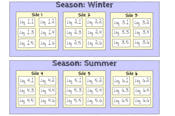
- Within each of the two Seasons, there were three separate Sites (Sites not repeatidly measured across Seasons).
- Within each of the Sites, six logs were selected (haphazardly) from which the number of flatworms were counted.
curdies <- read.csv("../downloads/data/curdies.csv", strip.white = T)
head(curdies)
  SEASON SITE   DUGESIA   S4DUGES
1 WINTER    1 0.6476829 0.8970995
2 WINTER    1 6.0961516 1.5713175
3 WINTER    1 1.3105639 1.0699526
4 WINTER    1 1.7252788 1.1460797
5 WINTER    1 1.4593867 1.0991136
6 WINTER    1 1.0575610 1.0140897
-
The SITE variable is supposed to represent a random factorial variable (which site).
However, because the contents of this variable are numbers, R initially treats them as numbers, and therefore considers the variable to be numeric rather than categorical.
In order to force R to treat this variable as a factor (categorical) it is necessary to first
convert this numeric variable into a factor (HINT)
.
Show code
curdies$SITE <- as.factor(curdies$SITE)
Notice the data set - each of the nested factors is labelled differently - there can be no replicate for the random (nesting) factor.
- What are the main hypotheses being tested?
- H0 Effect 1:
- H0 Effect 2:
- H0 Effect 1:
- In the table below, list the assumptions of nested ANOVA along with how violations of each assumption are diagnosed and/or the risks of violations are minimized.
Assumption Diagnostic/Risk Minimization I. II. III. - Check these assumptions
(HINT).
Show codeNote that for the effects of SEASON (Factor A in a nested model) there are only three values for each of the two season types. Therefore, boxplots are of limited value! Is there however, any evidence of violations of the assumptions (HINT)?
library(tidyverse)
curdies.ag <- curdies %>% group_by(SEASON, SITE) %>% summarize_if(is.numeric, mean)
Show codeboxplot(DUGESIA ~ SEASON, curdies.ag)
 Show ggplot code(Y or N)
library(ggplot2)
ggplot(curdies.ag, aes(y = DUGESIA, x = SEASON)) + geom_boxplot()

If so, assess whether a transformation will address the violations (HINT) and then make the appropriate corrections.Show codelibrary(tidyverse) curdies.ag <- curdies %>% group_by(SEASON, SITE) %>% summarize(S4DUGES = mean(DUGESIA^0.25, na.rm = TRUE))
Error in summarize(., S4DUGES = mean(DUGESIA^0.25, na.rm = TRUE)): argument "by" is missing, with no default
ggplot(curdies.ag, aes(y = S4DUGES, x = SEASON)) + geom_boxplot()

-
For each of the tests, state which error (or residual) term (state as Mean Square) will be used as the nominator and denominator to calculate the F ratio.
Also include degrees of freedom associated with each term.
Note this is a somewhat outdated procedure as there is far from
consensus about the most appropriate estimate of denominator degrees of freedom. Nevertheless, it sometimes helps to visualize the model hierarchy this way.
Effect Nominator (Mean Sq, df) Denominator (Mean Sq, df) SEASON SITE -
If there is no evidence of violations, fit the model;
S4DUGES = SEASON + SITE + CONSTANT
using a nested ANOVA (HINT). Fill (HINT) out the table below, make sure that you have treated SITE as a random factor when compiling the overall results.Show traditional codecurdies.aov <- aov(S4DUGES ~ SEASON + Error(SITE), data = curdies) summary(curdies.aov)
Error: SITE Df Sum Sq Mean Sq F value Pr(>F) SEASON 1 5.571 5.571 34.5 0.0042 ** Residuals 4 0.646 0.161 --- Signif. codes: 0 '***' 0.001 '**' 0.01 '*' 0.05 '.' 0.1 ' ' 1 Error: Within Df Sum Sq Mean Sq F value Pr(>F) Residuals 30 4.556 0.1519summary(lm(curdies.aov))
Call: lm(formula = curdies.aov) Residuals: Min 1Q Median 3Q Max -0.3811 -0.2618 -0.1381 0.1652 0.9023 Coefficients: (1 not defined because of singularities) Estimate Std. Error t value Pr(>|t|) (Intercept) 0.3811 0.1591 2.396 0.02303 * SEASONWINTER 0.7518 0.2250 3.342 0.00224 ** SITE2 0.1389 0.2250 0.618 0.54156 SITE3 -0.2651 0.2250 -1.178 0.24798 SITE4 -0.0303 0.2250 -0.135 0.89376 SITE5 -0.2007 0.2250 -0.892 0.37955 SITE6 NA NA NA NA --- Signif. codes: 0 '***' 0.001 '**' 0.01 '*' 0.05 '.' 0.1 ' ' 1 Residual standard error: 0.3897 on 30 degrees of freedom Multiple R-squared: 0.5771, Adjusted R-squared: 0.5066 F-statistic: 8.188 on 5 and 30 DF, p-value: 5.718e-05library(gmodels) ci(lm(curdies.aov))
                Estimate    CI lower  CI upper Std. Error     p-value
(Intercept)   0.38112230  0.05622464 0.7060200  0.1590863 0.023031342
SEASONWINTER  0.75181980  0.29234512 1.2112945  0.2249821 0.002241587
SITE2         0.13892772 -0.32054697 0.5984024  0.2249821 0.541560453
SITE3        -0.26507142 -0.72454610 0.1944033  0.2249821 0.247982761
SITE4        -0.03030097 -0.48977565 0.4291737  0.2249821 0.893763096
SITE5        -0.20066007 -0.66013475 0.2588146  0.2249821 0.379548177
Show lme codelibrary(nlme) # Fit random intercept model curdies.lme <- lme(S4DUGES ~ SEASON, random = ~1 | SITE, data = curdies, method = "REML") # Fit random intercept and slope model curdies.lme1 <- lme(S4DUGES ~ SEASON, random = ~SEASON | SITE, data = curdies, method = "REML") AIC(curdies.lme, curdies.lme1)
             df      AIC
curdies.lme   4 46.42966
curdies.lme1  6 50.10884
anova(curdies.lme, curdies.lme1)
             Model df      AIC     BIC    logLik   Test   L.Ratio p-value
curdies.lme      1  4 46.42966 52.5351 -19.21483
curdies.lme1     2  6 50.10884 59.2670 -19.05442 1 vs 2 0.3208206  0.8518
# Random intercepts and slope model does not fit the data better Use simpler random intercepts model
curdies.lme <- update(curdies.lme, method = "REML")

summary(curdies.lme)
Linear mixed-effects model fit by REML
 Data: curdies
       AIC     BIC    logLik
  46.42966 52.5351 -19.21483

Random effects:
 Formula: ~1 | SITE
        (Intercept)  Residual
StdDev:  0.04008595 0.3896804

Fixed effects: S4DUGES ~ SEASON
                 Value  Std.Error DF  t-value p-value
(Intercept)  0.3041353 0.09471949 30 3.210905  0.0031
SEASONWINTER 0.7867589 0.13395359  4 5.873369  0.0042
 Correlation:
             (Intr)
SEASONWINTER -0.707

Standardized Within-Group Residuals:
       Min         Q1        Med         Q3        Max
-1.2064783 -0.7680513 -0.2480589  0.3531126  2.3209353

Number of Observations: 36
Number of Groups: 6
# Calculate the confidence interval for the effect size of the main effect of season intervals(curdies.lme)
Approximate 95% confidence intervals

 Fixed effects:
                 lower      est.     upper
(Intercept)  0.1106923 0.3041353 0.4975783
SEASONWINTER 0.4148441 0.7867589 1.1586737
attr(,"label")
[1] "Fixed effects:"

 Random Effects:
  Level: SITE
                       lower       est.    upper
sd((Intercept)) 1.879311e-07 0.04008595 8550.386

 Within-group standard error:
    lower      est.     upper
0.3025657 0.3896804 0.5018771
# unique(confint(curdies.lme,'SEASONWINTER')[[1]]) Examine the ANOVA table with Type I (sequential) # SS anova(curdies.lme)
            numDF denDF   F-value p-value
(Intercept)     1    30 108.45712  <.0001
SEASON          1     4  34.49647  0.0042
Show lmer codelibrary(lme4) # Fit random intercepts model curdies.lmer <- lmer(S4DUGES ~ SEASON + (1 | SITE), data = curdies, REML = TRUE) # Fit random intercepts and slope model curdies.lmer1 <- lmer(S4DUGES ~ SEASON + (SEASON | SITE), data = curdies, REML = TRUE) AIC(curdies.lmer, curdies.lmer1)
              df      AIC
curdies.lmer   4 46.42966
curdies.lmer1  6 50.10884
anova(curdies.lmer, curdies.lmer1)
Data: curdies Models: curdies.lmer: S4DUGES ~ SEASON + (1 | SITE) curdies.lmer1: S4DUGES ~ SEASON + (SEASON | SITE) Df AIC BIC logLik deviance Chisq Chi Df Pr(>Chisq) curdies.lmer 4 40.519 46.853 -16.259 32.519 curdies.lmer1 6 44.478 53.979 -16.239 32.478 0.0412 2 0.9796summary(curdies.lmer)
Linear mixed model fit by REML ['lmerMod'] Formula: S4DUGES ~ SEASON + (1 | SITE) Data: curdies REML criterion at convergence: 38.4 Scaled residuals: Min 1Q Median 3Q Max -1.2065 -0.7681 -0.2481 0.3531 2.3209 Random effects: Groups Name Variance Std.Dev. SITE (Intercept) 0.001607 0.04009 Residual 0.151851 0.38968 Number of obs: 36, groups: SITE, 6 Fixed effects: Estimate Std. Error t value (Intercept) 0.30414 0.09472 3.211 SEASONWINTER 0.78676 0.13395 5.873 Correlation of Fixed Effects: (Intr) SEASONWINTE -0.707anova(curdies.lmer)
Analysis of Variance Table
       Df Sum Sq Mean Sq F value
SEASON  1 5.2383  5.2383  34.496
# Calculate the confidence interval for the effect size of the main effect of season confint(curdies.lmer)
                 2.5 %    97.5 %
.sig01       0.0000000 0.2278516
.sigma       0.3067343 0.4881844
(Intercept)  0.1237447 0.4825650
SEASONWINTER 0.5316481 1.0418697
# Perform SAS-like p-value calculations (requires the lmerTest and pbkrtest package)
library(lmerTest)
curdies.lmer <- lmer(S4DUGES ~ SEASON + (1 | SITE), data = curdies)
summary(curdies.lmer)
Linear mixed model fit by REML t-tests use Satterthwaite approximations to degrees of freedom [ lmerMod] Formula: S4DUGES ~ SEASON + (1 | SITE) Data: curdies REML criterion at convergence: 38.4 Scaled residuals: Min 1Q Median 3Q Max -1.2065 -0.7681 -0.2481 0.3531 2.3209 Random effects: Groups Name Variance Std.Dev. SITE (Intercept) 0.001607 0.04009 Residual 0.151851 0.38968 Number of obs: 36, groups: SITE, 6 Fixed effects: Estimate Std. Error df t value Pr(>|t|) (Intercept) 0.30414 0.09472 4.00000 3.211 0.0326 * SEASONWINTER 0.78676 0.13395 4.00000 5.873 0.0042 ** --- Signif. codes: 0 '***' 0.001 '**' 0.01 '*' 0.05 '.' 0.1 ' ' 1 Correlation of Fixed Effects: (Intr) SEASONWINTE -0.707anova(curdies.lmer) # Satterthwaite denominator df method
Analysis of Variance Table of type III with Satterthwaite approximation for degrees of freedom Sum Sq Mean Sq NumDF DenDF F.value Pr(>F) SEASON 5.2383 5.2383 1 4 34.496 0.004198 ** --- Signif. codes: 0 '***' 0.001 '**' 0.01 '*' 0.05 '.' 0.1 ' ' 1anova(curdies.lmer, ddf = "Kenward-Roger") # Kenward-Roger denominator df method
Analysis of Variance Table of type III  with  Kenward-Roger
approximation for degrees of freedom
       Sum Sq Mean Sq NumDF DenDF F.value   Pr(>F)
SEASON 5.2383  5.2383     1     4  34.496 0.004198 **
---
Signif. codes:  0 '***' 0.001 '**' 0.01 '*' 0.05 '.' 0.1 ' ' 1
# Examine the effect season via a likelihood ratio test curdies.lmer1 <- lmer(S4DUGES ~ SEASON + (1 | SITE), data = curdies, REML = F) curdies.lmer2 <- lmer(S4DUGES ~ 1 + (SEASON | SITE), data = curdies, REML = F) anova(curdies.lmer1, curdies.lmer2, test = "F")
Data: curdies
Models:
object: S4DUGES ~ SEASON + (1 | SITE)
..1: S4DUGES ~ 1 + (SEASON | SITE)
       Df    AIC    BIC  logLik deviance Chisq Chi Df Pr(>Chisq)
object  4 40.519 46.853 -16.259   32.519
..1     5 51.780 59.698 -20.890   41.780     0      1          1
Show glmmTMB codelibrary(glmmTMB) # Fit random intercepts model curdies.glmmTMB <- glmmTMB(S4DUGES ~ SEASON + (1 | SITE), data = curdies) # Fit random intercepts and slope model curdies.glmmTMB1 <- glmmTMB(S4DUGES ~ SEASON + (SEASON | SITE), data = curdies) AIC(curdies.glmmTMB, curdies.glmmTMB1)
                 df      AIC
curdies.glmmTMB   4 40.51893
curdies.glmmTMB1  6       NA
anova(curdies.glmmTMB, curdies.glmmTMB1)
Data: curdies Models: curdies.glmmTMB: S4DUGES ~ SEASON + (1 | SITE), zi=~0, disp=~1 curdies.glmmTMB1: S4DUGES ~ SEASON + (SEASON | SITE), zi=~0, disp=~1 Df AIC BIC logLik deviance Chisq Chi Df Pr(>Chisq) curdies.glmmTMB 4 40.519 46.853 -16.259 32.519 curdies.glmmTMB1 6 2summary(curdies.glmmTMB)
 Family: gaussian  ( identity )
Formula:          S4DUGES ~ SEASON + (1 | SITE)
Data: curdies

     AIC      BIC   logLik deviance df.resid
    40.5     46.9    -16.3     32.5       32

Random effects:

Conditional model:
 Groups   Name        Variance  Std.Dev.
 SITE     (Intercept) 6.781e-11 8.235e-06
 Residual             1.445e-01 3.801e-01
Number of obs: 36, groups:  SITE, 6

Dispersion estimate for gaussian family (sigma^2): 0.144

Conditional model:
             Estimate Std. Error z value Pr(>|z|)
(Intercept)   0.30414    0.08959   3.395 0.000687 ***
SEASONWINTER  0.78676    0.12670   6.209 5.32e-10 ***
---
Signif. codes:  0 '***' 0.001 '**' 0.01 '*' 0.05 '.' 0.1 ' ' 1
# Calculate the confidence interval for the effect size of the main effect of season confint(curdies.glmmTMB)
                                  2.5 %    97.5 %     Estimate
cond.(Intercept)              0.1285353 0.4797353 3.041353e-01
cond.SEASONWINTER             0.5384230 1.0350948 7.867589e-01
cond.Std.Dev.SITE.(Intercept) 0.0000000       Inf 8.234920e-06
sigma                         0.3017155 0.4788812 3.801130e-01
- Check the model diagnostics
- Residual plot
Show traditional codepar(mfrow = c(2, 2)) plot(lm(curdies.aov))
 Show lme code
plot(curdies.lme)

qqnorm(resid(curdies.lme))
qqline(resid(curdies.lme))

library(sjPlot)
plot_grid(plot_model(curdies.lme, type = "diag"))
 Show lmer code
plot(curdies.lmer)

plot(fitted(curdies.lmer), residuals(curdies.lmer, type = "pearson", scaled = TRUE))

ggplot(fortify(curdies.lmer), aes(y = .scresid, x = .fitted)) + geom_point()

qq.line = function(x) {
    # following four lines from base R's qqline()
    y <- quantile(x[!is.na(x)], c(0.25, 0.75))
    x <- qnorm(c(0.25, 0.75))
    slope <- diff(y)/diff(x)
    int <- y[1L] - slope * x[1L]
    return(c(int = int, slope = slope))
}
QQline = qq.line(fortify(curdies.lmer)$.scresid)
ggplot(fortify(curdies.lmer), aes(sample = .scresid)) + stat_qq() + geom_abline(intercept = QQline[1],
    slope = QQline[2])

qqnorm(resid(curdies.lmer))
qqline(resid(curdies.lmer))

library(sjPlot)
plot_grid(plot_model(curdies.lmer, type = "diag"))
 Show glmmTMB code
ggplot(data = NULL, aes(y = resid(curdies.glmmTMB, type = "pearson"),
    x = fitted(curdies.glmmTMB))) + geom_point()

QQline = qq.line(resid(curdies.glmmTMB, type = "pearson"))
ggplot(data = NULL, aes(sample = resid(curdies.glmmTMB, type = "pearson"))) +
    stat_qq() + geom_abline(intercept = QQline[1], slope = QQline[2])

- For each of the tests, state which error (or residual) term (state as Mean Square) will be used as the nominator and denominator to calculate the F ratio. Also include degrees of freedom associated with each term.
Source of variation df Mean Sq F-ratio P-value SEASON SITE Residuals
Estimate Mean Lower 95% CI Upper 95% CI Summer Effect size (Winter-Summer) - Lets produce a quick partial (marginal) effects plot to represent
the model.
Show lme code
library(effects)
plot(allEffects(curdies.lme))

library(sjPlot)
plot_model(curdies.lme, type = "eff", terms = "SEASON")
 Show lmer code
library(effects)
plot(allEffects(curdies.lmer))

library(sjPlot)
plot_model(curdies.lmer, type = "eff", terms = "SEASON")
 Show glmmTMB code
library(ggeffects)
# observation level effects averaged across margins
p = ggaverage(curdies.glmmTMB, terms = "SEASON")
p = cbind(p, SEASON = levels(curdies$SEASON))
ggplot(p, aes(y = predicted, x = SEASON)) + geom_pointrange(aes(ymin = conf.low, ymax = conf.high))

# marginal effects
p = ggpredict(curdies.glmmTMB, terms = "SEASON")
p = cbind(p, SEASON = levels(curdies$SEASON))
ggplot(p, aes(y = predicted, x = SEASON)) + geom_pointrange(aes(ymin = conf.low, ymax = conf.high))

- Where is the major variation in numbers of flatworms? Between (seasons, sites or stones)?
Show code for lme
library(nlme) nlme:::VarCorr(curdies.lme)
SITE = pdLogChol(1) Variance StdDev (Intercept) 0.001606883 0.04008595 Residual 0.151850778 0.38968035library(MuMIn) r.squaredGLMM(curdies.lme)
R2m R2c 0.509134 0.514274
Show code for lmeVarCorr(curdies.lmer)
Groups Name Std.Dev. SITE (Intercept) 0.040086 Residual 0.389680
library(MuMIn) r.squaredGLMM(curdies.lmer)
R2m R2c 0.5091341 0.5142739
Show code for glmmTMBVarCorr(curdies.glmmTMB)
Conditional model: Groups Name Std.Dev. SITE (Intercept) 8.2349e-06 Residual 3.8011e-01
source(system.file("misc/rsqglmm.R", package = "glmmTMB")) my_rsq(curdies.glmmTMB)
$family [1] "gaussian" $link [1] "identity" $Marginal [1] 0.5241769 $Conditional [1] 0.5241769
- Finally, construct an appropriate summary figure
to accompany the above analyses. Note that this should use the correct replicates for depicting error.
Show lme code
library(effects) curdies.eff = as.data.frame(Effect("SEASON", curdies.lme)) ggplot(curdies.eff, aes(y = fit^4, x = SEASON)) + geom_pointrange(aes(ymin = lower^4, ymax = upper^4)) + scale_y_continuous("Mean number of Dugesia per stone") + theme_classic()

# OR manually newdata <- data.frame(SEASON = levels(curdies$SEASON)) Xmat <- model.matrix(~SEASON, data = newdata) coefs <- fixef(curdies.lme) fit <- as.vector(coefs %*% t(Xmat)) se <- sqrt(diag(Xmat %*% vcov(curdies.lme) %*% t(Xmat))) q = qt(0.975, df = nrow(curdies.lme$data) - length(coefs) - 2) newdata <- cbind(newdata, fit = (fit)^4, lower = (fit - 2 * se)^4, upper = (fit + 2 * se)^4) ggplot(newdata, aes(y = fit, x = SEASON)) + geom_errorbar(aes(ymin = lower, ymax = upper), width = 0.05) + geom_point(size = 2) + scale_y_continuous("Mean number of Dugesia per stone") + theme_classic() + theme(axis.title.x = element_blank(), axis.title.y = element_text(vjust = 2, size = rel(1.25)), panel.margin = unit(c(0.5, 0.5, 0.5, 2), "lines"))
 Show lmer code
library(effects) curdies.eff = as.data.frame(Effect("SEASON", curdies.lmer)) ggplot(curdies.eff, aes(y = fit^4, x = SEASON)) + geom_pointrange(aes(ymin = lower^4, ymax = upper^4)) + scale_y_continuous("Mean number of Dugesia per stone") + theme_classic()

# OR manually newdata <- data.frame(SEASON = levels(curdies$SEASON)) Xmat <- model.matrix(~SEASON, data = newdata) coefs <- fixef(curdies.lmer) fit <- as.vector(coefs %*% t(Xmat)) se <- sqrt(diag(Xmat %*% vcov(curdies.lmer) %*% t(Xmat))) q = qt(0.975, df = df.residual(curdies.lmer)) newdata <- cbind(newdata, fit = (fit)^4, lower = (fit - 2 * se)^4, upper = (fit + 2 * se)^4) ggplot(newdata, aes(y = fit, x = SEASON)) + geom_errorbar(aes(ymin = lower, ymax = upper), width = 0.05) + geom_point(size = 2) + scale_y_continuous("Mean number of Dugesia per stone") + theme_classic() + theme(axis.title.x = element_blank(), axis.title.y = element_text(vjust = 2, size = rel(1.25)), panel.margin = unit(c(0.5, 0.5, 0.5, 2), "lines"))
 Show glmmTMB code
newdata <- data.frame(SEASON = levels(curdies$SEASON)) Xmat <- model.matrix(~SEASON, data = newdata) coefs <- fixef(curdies.glmmTMB)[[1]] fit <- as.vector(coefs %*% t(Xmat)) se <- sqrt(diag(Xmat %*% vcov(curdies.glmmTMB)[[1]] %*% t(Xmat))) q = qt(0.975, df = df.residual(curdies.glmmTMB)) newdata <- cbind(newdata, fit = (fit)^4, lower = (fit - 2 * se)^4, upper = (fit + 2 * se)^4) ggplot(newdata, aes(y = fit, x = SEASON)) + geom_errorbar(aes(ymin = lower, ymax = upper), width = 0.05) + geom_point(size = 2) + scale_y_continuous("Mean number of Dugesia per stone") + theme_classic() + theme(axis.title.x = element_blank(), axis.title.y = element_text(vjust = 2, size = rel(1.25)), panel.margin = unit(c(0.5, 0.5, 0.5, 2), "lines"))

Note, this tutorial is focussed on linear mixed effects against a Gaussian and therefore we will normalized our response (via forth-root transformation). Given that the data are counts. Arguably, it would be more appropriate to model the raw data against a poisson distribution. We will do so in Tutorial 11.2a