Jump to main navigation


Workshop 11.5a - Poisson regression and log-linear models

23 April 2011

Basic χ2 references

  • Logan (2010) - Chpt 16-17
  • Quinn & Keough (2002) - Chpt 13-14

Poisson t-test

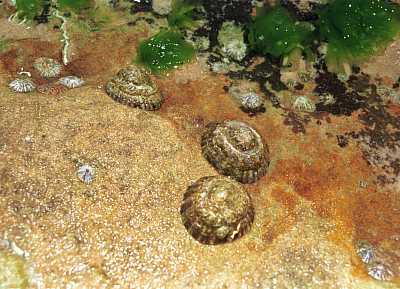
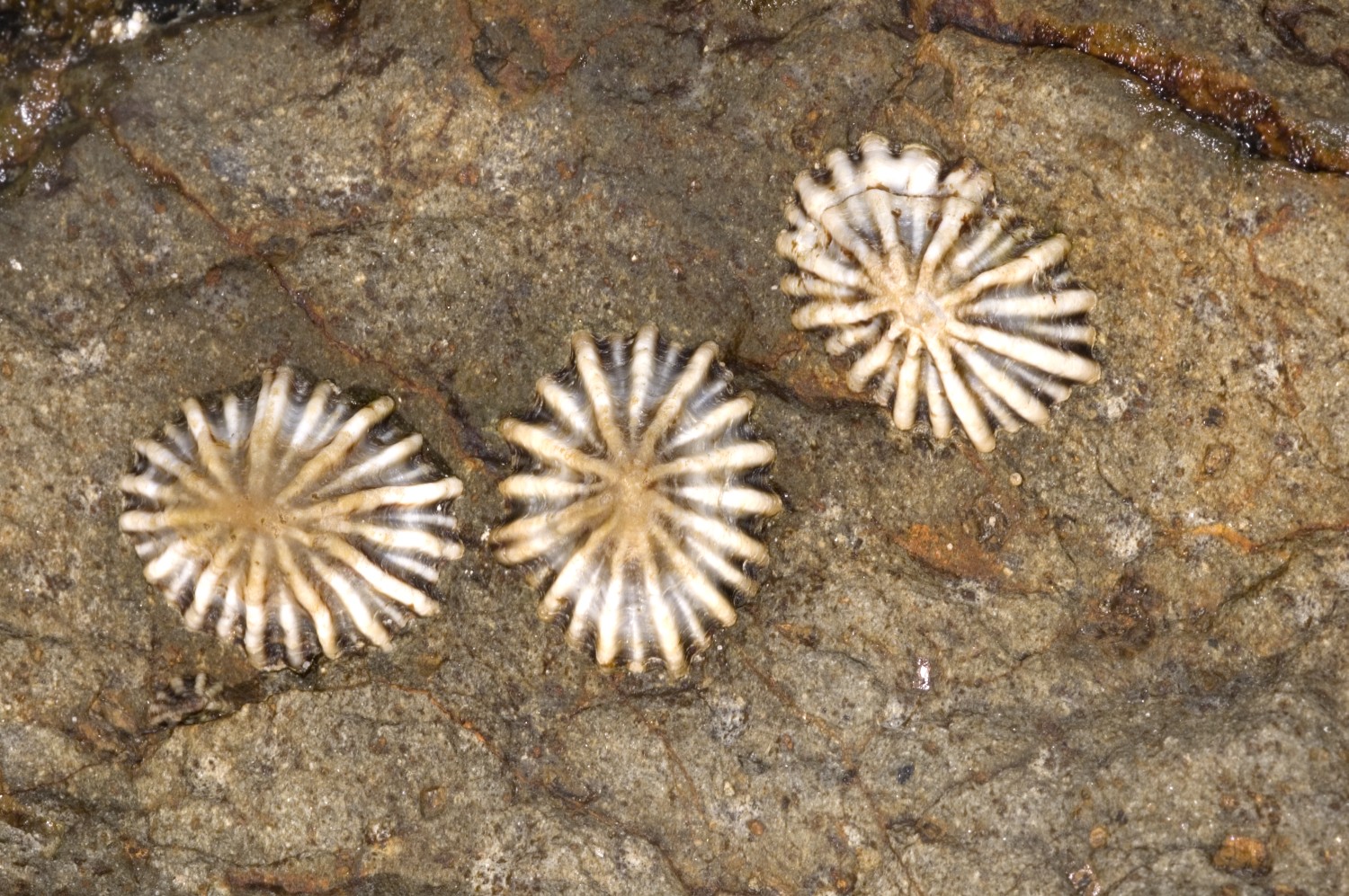
A marine ecologist was interested in examining the effects of wave exposure on the abundance of the striped limpet Siphonaria diemenensis on rocky intertidal shores. To do so, a single quadrat was placed on 10 exposed (to large waves) shores and 10 sheltered shores. From each quadrat, the number of Siphonaria diemenensis were counted.

Download Limpets data set
Format of limpets.csv data files
CountShore
1sheltered
3sheltered
2sheltered
1sheltered
4sheltered
......

ShoreCategorical description of the shore type (sheltered or exposed) - Predictor variable
CountNumber of limpets per quadrat - Response variable
turf

Open the limpet data set.

Show code
> limpets <- read.table('../downloads/data/limpets.csv', header=T, sep=',', strip.white=T)
> limpets
   Count     Shore
1      2 sheltered
2      2 sheltered
3      0 sheltered
4      6 sheltered
5      0 sheltered
6      3 sheltered
7      3 sheltered
8      0 sheltered
9      1 sheltered
10     2 sheltered
11     5   exposed
12     3   exposed
13     6   exposed
14     3   exposed
15     4   exposed
16     7   exposed
17    10   exposed
18     3   exposed
19     5   exposed
20     2   exposed

The design is clearly a t-test as we are interested in comparing two population means (mean number of striped limpets on exposed and sheltered shores). Recall that a parametric t-test assumes that the residuals (and populations from which the samples are drawn) are normally distributed and equally varied.

  1. Is there any evidence that these assumptions have been violated?
    Show code
    > boxplot(Count~Shore, data=limpets)
    
    plot of chunk Q1_1
    1. The assumption of normality has been violated?
    2. The assumption of homogeneity of variance has been violated?
  2. At this point we could transform the data in an attempt to satisfy normality and homogeneity of variance. However, the analyses are then not on the scale of the data and thus the conclusions also pertain to a different scale. Furthermore, linear modelling on transformed count data is generally not as effective as modelling count data with a Poisson distribution.

  3. Lets instead we fit the same model with a Poisson distribution. $$log(\mu) = \beta_0+\beta1Shore_i+\epsilon_i, \hspace{1cm} \epsilon \sim Poisson(\lambda)$$
    Show code
    > limpets.glm <- glm(Count~Shore, family=poisson, data=limpets)
    
    1. Check the model for lack of fit via:
      • Pearson Χ2
        Show code
        > limpets.resid <- sum(resid(limpets.glm, type="pearson")^2)
        > 1-pchisq(limpets.resid, limpets.glm$df.resid)
        
        [1] 0.07875
        
        > #No evidence of a lack of fit
        
      • Deviance (G2)
        Show code
        > 1-pchisq(limpets.glm$deviance, limpets.glm$df.resid)
        
        [1] 0.05287
        
        > #No evidence of a lack of fit
        
      • Standardized residuals (plot)
        Show code
        > plot(limpets.glm)
        
        plot of chunk Q1_2d
        plot of chunk Q1_2d
        plot of chunk Q1_2d
        plot of chunk Q1_2d
    2. Estimate the dispersion parameter to evaluate over dispersion in the fitted model
      • Via Pearson residuals
        Show code
        > limpets.resid/limpets.glm$df.resid
        
        [1] 1.501
        
        > #No evidence of over dispersion
        
      • Via deviance
        Show code
        > limpets.glm$deviance/limpets.glm$df.resid
        
        [1] 1.591
        
        > #No evidence of over dispersion
        
    3. Compare the expected number of zeros to the actual number of zeros to determine whether the model might be zero inflated.
      • Calculate the proportion of zeros in the data
        Show code
        > limpets.tab<-table(limpets$Count==0)
        > limpets.tab/sum(limpets.tab)
        
        FALSE  TRUE 
         0.85  0.15 
        
      • Now work out the proportion of zeros we would expect from a Poisson distribution with a lambda equal to the mean count of limpets in this study.
        Show code
        > limpets.mu <- mean(limpets$Count)
        > cnts <-rpois(1000,limpets.mu)
        > limpets.tab<-table(cnts==0)
        > limpets.tab/sum(limpets.tab)
        
        FALSE  TRUE 
        0.955 0.045 
        
        There are not substantially higher proportion of zeros than would be expected. The data a slightly zero inflated.
  4. We can now test the null hypothesis that there is no effect of shore type on the abundance of striped limpets;
    1. Wald z-tests (these are equivalent to t-tests)
    2. Show code
      > summary(limpets.glm)
      
      Call:
      glm(formula = Count ~ Shore, family = poisson, data = limpets)
      
      Deviance Residuals: 
          Min       1Q   Median       3Q      Max  
      -1.9494  -0.8832   0.0719   0.5791   2.3662  
      
      Coefficients:
                     Estimate Std. Error z value Pr(>|z|)    
      (Intercept)       1.569      0.144   10.87  < 2e-16 ***
      Shoresheltered   -0.927      0.271   -3.42  0.00063 ***
      ---
      Signif. codes:  0 '***' 0.001 '**' 0.01 '*' 0.05 '.' 0.1 ' ' 1
      
      (Dispersion parameter for poisson family taken to be 1)
      
          Null deviance: 41.624  on 19  degrees of freedom
      Residual deviance: 28.647  on 18  degrees of freedom
      AIC: 85.57
      
      Number of Fisher Scoring iterations: 5
      
    3. Wald Chisq-test. Note that Chisq = z2
    4. Show code
      > library(car)
      > Anova(limpets.glm,test.statistic="Wald")
      
      Analysis of Deviance Table (Type II tests)
      
      Response: Count
                Df Chisq Pr(>Chisq)    
      Shore      1  11.7    0.00063 ***
      Residuals 18                     
      ---
      Signif. codes:  0 '***' 0.001 '**' 0.01 '*' 0.05 '.' 0.1 ' ' 1
      
    5. Likelihood ratio test (LRT), analysis of deviance Chisq-tests (these are equivalent to ANOVA)
    6. Show code
      > limpets.glmN <- glm(Count~1, family=poisson, data=limpets)
      > anova(limpets.glmN, limpets.glm, test="Chisq")
      
      Analysis of Deviance Table
      
      Model 1: Count ~ 1
      Model 2: Count ~ Shore
        Resid. Df Resid. Dev Df Deviance Pr(>Chi)    
      1        19       41.6                         
      2        18       28.6  1       13  0.00032 ***
      ---
      Signif. codes:  0 '***' 0.001 '**' 0.01 '*' 0.05 '.' 0.1 ' ' 1
      
      > # OR
      > anova(limpets.glm, test="Chisq")
      
      Analysis of Deviance Table
      
      Model: poisson, link: log
      
      Response: Count
      
      Terms added sequentially (first to last)
      
      
            Df Deviance Resid. Df Resid. Dev Pr(>Chi)    
      NULL                     19       41.6             
      Shore  1       13        18       28.6  0.00032 ***
      ---
      Signif. codes:  0 '***' 0.001 '**' 0.01 '*' 0.05 '.' 0.1 ' ' 1
      
      > # OR
      > Anova(limpets.glm, test.statistic="LR")
      
      Analysis of Deviance Table (Type II tests)
      
      Response: Count
            LR Chisq Df Pr(>Chisq)    
      Shore       13  1    0.00032 ***
      ---
      Signif. codes:  0 '***' 0.001 '**' 0.01 '*' 0.05 '.' 0.1 ' ' 1
      
  5. And for those who do not suffer a p-value affliction, we can alternatively (or in addition) calculate the confidence intervals for the estimated parameters.
    Show code
    > library(gmodels)
    > ci(limpets.glm)
    
                   Estimate CI lower CI upper Std. Error   p-value
    (Intercept)      1.5686    1.265   1.8719     0.1443 1.643e-27
    Shoresheltered  -0.9268   -1.496  -0.3573     0.2710 6.280e-04
    
  6. Had we have been concerned about overdispersion, we could have alternatively fit a model against either a quasipoisson or negative binomial distribution.
    Show code
    > limpets.glmQ <- glm(Count~Shore, family=quasipoisson, data=limpets)
    > summary(limpets.glmQ)
    
    Call:
    glm(formula = Count ~ Shore, family = quasipoisson, data = limpets)
    
    Deviance Residuals: 
        Min       1Q   Median       3Q      Max  
    -1.9494  -0.8832   0.0719   0.5791   2.3662  
    
    Coefficients:
                   Estimate Std. Error t value Pr(>|t|)    
    (Intercept)       1.569      0.177    8.87  5.5e-08 ***
    Shoresheltered   -0.927      0.332   -2.79    0.012 *  
    ---
    Signif. codes:  0 '***' 0.001 '**' 0.01 '*' 0.05 '.' 0.1 ' ' 1
    
    (Dispersion parameter for quasipoisson family taken to be 1.501)
    
        Null deviance: 41.624  on 19  degrees of freedom
    Residual deviance: 28.647  on 18  degrees of freedom
    AIC: NA
    
    Number of Fisher Scoring iterations: 5
    
    > anova(limpets.glmQ, test="Chisq")
    
    Analysis of Deviance Table
    
    Model: quasipoisson, link: log
    
    Response: Count
    
    Terms added sequentially (first to last)
    
    
          Df Deviance Resid. Df Resid. Dev Pr(>Chi)   
    NULL                     19       41.6            
    Shore  1       13        18       28.6   0.0033 **
    ---
    Signif. codes:  0 '***' 0.001 '**' 0.01 '*' 0.05 '.' 0.1 ' ' 1
    
    > library(MASS)
    > limpets.nb <- glm.nb(Count~Shore, data=limpets)
    > summary(limpets.nb)
    
    Call:
    glm.nb(formula = Count ~ Shore, data = limpets, init.theta = 15.58558116, 
        link = log)
    
    Deviance Residuals: 
        Min       1Q   Median       3Q      Max  
    -1.8936  -0.7849   0.0678   0.5143   2.1691  
    
    Coefficients:
                   Estimate Std. Error z value Pr(>|z|)    
    (Intercept)       1.569      0.165    9.50   <2e-16 ***
    Shoresheltered   -0.927      0.294   -3.15   0.0016 ** 
    ---
    Signif. codes:  0 '***' 0.001 '**' 0.01 '*' 0.05 '.' 0.1 ' ' 1
    
    (Dispersion parameter for Negative Binomial(15.59) family taken to be 1)
    
        Null deviance: 35.224  on 19  degrees of freedom
    Residual deviance: 24.470  on 18  degrees of freedom
    AIC: 87.15
    
    Number of Fisher Scoring iterations: 1
    
    
                  Theta:  15.6 
              Std. Err.:  28.8 
    
     2 x log-likelihood:  -81.15 
    
    > anova(limpets.nb, test="Chisq")
    
    Analysis of Deviance Table
    
    Model: Negative Binomial(15.59), link: log
    
    Response: Count
    
    Terms added sequentially (first to last)
    
    
          Df Deviance Resid. Df Resid. Dev Pr(>Chi)   
    NULL                     19       35.2            
    Shore  1     10.8        18       24.5    0.001 **
    ---
    Signif. codes:  0 '***' 0.001 '**' 0.01 '*' 0.05 '.' 0.1 ' ' 1
    

Poisson ANOVA (regression)

We once again return to a modified example from Quinn and Keough (2002). In Exercise 1 of Workshop 9.4a, we introduced an experiment by Day and Quinn (1989) that examined how rock surface type affected the recruitment of barnacles to a rocky shore. The experiment had a single factor, surface type, with 4 treatments or levels: algal species 1 (ALG1), algal species 2 (ALG2), naturally bare surfaces (NB) and artificially scraped bare surfaces (S). There were 5 replicate plots for each surface type and the response (dependent) variable was the number of newly recruited barnacles on each plot after 4 weeks.

Download Day data set
Format of day.csv data files
TREATBARNACLE
ALG127
....
ALG224
....
NB9
....
S12
....
TREATCategorical listing of surface types. ALG1 = algal species 1, ALG2 = algal species 2, NB = naturally bare surface, S = scraped bare surface.
BARNACLEThe number of newly recruited barnacles on each plot after 4 weeks.
Six-plated barnacle

Open
the day data file.
Show code
> day <- read.table('../downloads/data/day.csv', header=T, sep=',', strip.white=T)
> head(day)
  TREAT BARNACLE
1  ALG1       27
2  ALG1       19
3  ALG1       18
4  ALG1       23
5  ALG1       25
6  ALG2       24

We previously analysed these data with via a classic linear model (ANOVA) as the data appeared to conform to the linear model assumptions. Alternatively, we could analyse these data with a generalized linear model (Poisson error distribution). Note that as the boxplots were all fairly symmetrical and equally varied, and the sample means are well away from zero (in fact there are no zero's in the data) we might suspect that whether we fit the model as a linear or generalized linear model is probably not going to be of great consequence. Nevertheless, it does then provide a good comparison between the two frameworks.

  1. Using boxplots re-examine the assumptions of normality and homogeneity of variance. Note that when sample sizes are small (as is the case with this data set), these ANOVA assumptions cannot reliably be checked using boxplots since boxplots require at least 5 replicates (and preferably more), from which to calculate the median and quartiles. As with regression analysis, it is the assumption of homogeneity of variances (and in particular, whether there is a relationship between the mean and variance) that is of most concern for ANOVA.
    Show code
    > boxplot(BARNACLE~TREAT, data=day)
    
    plot of chunk Q2_1
  2. Fit the generalized linear model (GLM) relating the number of newly recruited barnacles to substrate type. $$log(\mu) = \beta_0+\beta1Treat_i+\epsilon_i, \hspace{1cm} \epsilon \sim Poisson(\lambda)$$
    Show code
    > day.glm<-glm(BARNACLE~TREAT, family=poisson,data=day)
    
    1. Check the model for lack of fit via:
      • Pearson Χ2
        Show code
        > day.resid <- sum(resid(day.glm, type="pearson")^2)
        > 1-pchisq(day.resid, day.glm$df.resid)
        
        [1] 0.3641
        
        > #No evidence of a lack of fit
        
      • Standardized residuals (plot)
        Show code
        > plot(day.glm)
        
        plot of chunk Q2_2b
        plot of chunk Q2_2b
        plot of chunk Q2_2b
        plot of chunk Q2_2b
    2. Estimate the dispersion parameter to evaluate over dispersion in the fitted model
      • Via Pearson residuals
        Show code
        > day.resid/day.glm$df.resid
        
        [1] 1.084
        
        > #No evidence of over dispersion
        
      • Via deviance
        Show code
        > day.glm$deviance/day.glm$df.resid
        
        [1] 1.076
        
        > #No evidence of over dispersion
        
    3. Compare the expected number of zeros to the actual number of zeros to determine whether the model might be zero inflated.
      • Calculate the proportion of zeros in the data
        Show code
        > day.tab<-table(day$Count==0)
        > day.tab/sum(day.tab)
        
        numeric(0)
        
      • Now work out the proportion of zeros we would expect from a Poisson distribution with a lambda equal to the mean count of day in this study.
        Show code
        > day.mu <- mean(day$Count)
        > cnts <-rpois(1000,day.mu)
        > day.tab<-table(cnts==0)
        > day.tab/sum(day.tab)
        
        numeric(0)
        
        Clearly there are not more zeros than expected so the data are not zero inflated.
  3. We can now test the null hypothesis that there is no effect of shore type on the abundance of striped day;
    1. Wald z-tests (these are equivalent to t-tests)
    2. Show code
      > summary(day.glm)
      
      Call:
      glm(formula = BARNACLE ~ TREAT, family = poisson, data = day)
      
      Deviance Residuals: 
         Min      1Q  Median      3Q     Max  
      -1.675  -0.652  -0.263   0.570   1.738  
      
      Coefficients:
                  Estimate Std. Error z value Pr(>|z|)    
      (Intercept)   3.1091     0.0945   32.90  < 2e-16 ***
      TREATALG2     0.2373     0.1264    1.88  0.06039 .  
      TREATNB      -0.4010     0.1492   -2.69  0.00720 ** 
      TREATS       -0.5288     0.1552   -3.41  0.00065 ***
      ---
      Signif. codes:  0 '***' 0.001 '**' 0.01 '*' 0.05 '.' 0.1 ' ' 1
      
      (Dispersion parameter for poisson family taken to be 1)
      
          Null deviance: 54.123  on 19  degrees of freedom
      Residual deviance: 17.214  on 16  degrees of freedom
      AIC: 120.3
      
      Number of Fisher Scoring iterations: 4
      
    3. Wald Chisq-test.
    4. Show code
      > library(car)
      > Anova(day.glm,test.statistic="Wald")
      
      Analysis of Deviance Table (Type II tests)
      
      Response: BARNACLE
                Df Chisq Pr(>Chisq)    
      TREAT      3    36    7.3e-08 ***
      Residuals 16                     
      ---
      Signif. codes:  0 '***' 0.001 '**' 0.01 '*' 0.05 '.' 0.1 ' ' 1
      
    5. Likelihood ratio test (LRT), analysis of deviance Chisq-tests (these are equivalent to ANOVA)
    6. Show code
      > day.glmN <- glm(BARNACLE~1, family=poisson, data=day)
      > anova(day.glmN, day.glm, test="Chisq")
      
      Analysis of Deviance Table
      
      Model 1: BARNACLE ~ 1
      Model 2: BARNACLE ~ TREAT
        Resid. Df Resid. Dev Df Deviance Pr(>Chi)    
      1        19       54.1                         
      2        16       17.2  3     36.9  4.8e-08 ***
      ---
      Signif. codes:  0 '***' 0.001 '**' 0.01 '*' 0.05 '.' 0.1 ' ' 1
      
      > # OR
      > anova(day.glm, test="Chisq")
      
      Analysis of Deviance Table
      
      Model: poisson, link: log
      
      Response: BARNACLE
      
      Terms added sequentially (first to last)
      
      
            Df Deviance Resid. Df Resid. Dev Pr(>Chi)    
      NULL                     19       54.1             
      TREAT  3     36.9        16       17.2  4.8e-08 ***
      ---
      Signif. codes:  0 '***' 0.001 '**' 0.01 '*' 0.05 '.' 0.1 ' ' 1
      
      > # OR
      > Anova(day.glm, test.statistic="LR")
      
      Analysis of Deviance Table (Type II tests)
      
      Response: BARNACLE
            LR Chisq Df Pr(>Chisq)    
      TREAT     36.9  3    4.8e-08 ***
      ---
      Signif. codes:  0 '***' 0.001 '**' 0.01 '*' 0.05 '.' 0.1 ' ' 1
      
  4. Lets now get the confidence intervals for the parameter estimates. Note these are still on the logs scale!
    Show code
    > library(gmodels)
    > ci(day.glm)
    
                Estimate CI lower CI upper Std. Error    p-value
    (Intercept)   3.1091  2.90875  3.30937    0.09449 1.977e-237
    TREATALG2     0.2373 -0.03058  0.50523    0.12638  6.039e-02
    TREATNB      -0.4010 -0.71731 -0.08471    0.14920  7.195e-03
    TREATS       -0.5288 -0.85781 -0.19988    0.15518  6.544e-04
    
  5. Although we have now established that there is a statistical difference between the group means, we do not yet know which group(s) are different from which other(s). For this data a Tukey's multiple comparison test (to determine which surface type groups are different from each other, in terms of number of barnacles) could be appropriate.
    Show code
    > library(multcomp)
    > summary(glht(day.glm,linfct=mcp(TREAT="Tukey")))
    
    	 Simultaneous Tests for General Linear Hypotheses
    
    Multiple Comparisons of Means: Tukey Contrasts
    
    
    Fit: glm(formula = BARNACLE ~ TREAT, family = poisson, data = day)
    
    Linear Hypotheses:
                     Estimate Std. Error z value Pr(>|z|)    
    ALG2 - ALG1 == 0    0.237      0.126    1.88   0.2353    
    NB - ALG1 == 0     -0.401      0.149   -2.69   0.0360 *  
    S - ALG1 == 0      -0.529      0.155   -3.41   0.0038 ** 
    NB - ALG2 == 0     -0.638      0.143   -4.47   <0.001 ***
    S - ALG2 == 0      -0.766      0.149   -5.14   <0.001 ***
    S - NB == 0        -0.128      0.169   -0.76   0.8723    
    ---
    Signif. codes:  0 '***' 0.001 '**' 0.01 '*' 0.05 '.' 0.1 ' ' 1
    (Adjusted p values reported -- single-step method)
    
  6. I am now in the mood to derive other parameters from the model:
    1. Cell (population) means
      Show code
      > day.means <- predict(day.glm,newdata=data.frame(TREAT=levels(day$TREAT)),se=T)
      > day.means <- data.frame(day.means[1],day.means[2])
      > rownames(day.means) <- levels(day$TREAT)
      > day.ci <- qt(0.975,day.glm$df.residual)*day.means[,2]
      > day.means <- data.frame(day.means,lwr=day.means[,1]-day.ci,upr=day.means[,1]+day.ci)
      > #On the scale of the response
      > day.means <- predict(day.glm,newdata=data.frame(TREAT=levels(day$TREAT)),se=T, type="response")
      > day.means <- data.frame(day.means[1],day.means[2])
      > rownames(day.means) <- levels(day$TREAT)
      > day.ci <- qt(0.975,day.glm$df.residual)*day.means[,2]
      > day.means <- data.frame(day.means,lwr=day.means[,1]-day.ci,upr=day.means[,1]+day.ci)
      > day.means
      
            fit se.fit    lwr   upr
      ALG1 22.4  2.117 17.913 26.89
      ALG2 28.4  2.383 23.348 33.45
      NB   15.0  1.732 11.328 18.67
      S    13.2  1.625  9.756 16.64
      
      > opar<-par(mar=c(4,5,1,1))
      > plot(BARNACLE~as.numeric(TREAT), data=day, ann=F, axes=F, type="n")
      > points(BARNACLE~as.numeric(TREAT), data=day, pch=16, col="grey80")
      > arrows(as.numeric(factor(rownames(day.means))),day.means$lwr,as.numeric(factor(rownames(day.means))), day.means$upr, ang=90, length=0.1, code=3)
      > points(day.means$fit~as.numeric(factor(rownames(day.means))), pch=16)
      > axis(1, at=as.numeric(factor(rownames(day.means))), labels=rownames(day.means))
      > mtext("Treatment",1, line=3, cex=1.2)
      > axis(2, las=1)
      > mtext("Number of newly recruited barnacles",2, line=3, cex=1.2)
      > box(bty="l")
      
      plot of chunk Q2_6
      Or the long way
      Show code
      > #On a link (log) scale 
      > cmat <- cbind(c(1,0,0,0),c(1,1,0,0),c(1,0,1,0),c(1,0,0,1))
      > day.mu<-t(day.glm$coef %*% cmat)
      > day.se <- sqrt(diag(t(cmat) %*% vcov(day.glm) %*% cmat))
      > day.means <- data.frame(fit=day.mu,se=day.se)
      > rownames(day.means) <- levels(day$TREAT)
      > day.ci <- qt(0.975,day.glm$df.residual)*day.se
      > day.means <- data.frame(day.means,lwr=day.mu-day.ci,upr=day.mu+day.ci)
      > #On a response scale 
      > cmat <- cbind(c(1,0,0,0),c(1,1,0,0),c(1,0,1,0),c(1,0,0,1))
      > day.mu<-t(day.glm$coef %*% cmat)
      > day.se <- sqrt(diag(t(cmat) %*% vcov(day.glm) %*% cmat))*abs(poisson()$mu.eta(day.mu))
      > day.mu<-exp(day.mu)
      > #OR
      > day.se <- sqrt(diag(vcov(day.glm) %*% cmat))*day.mu
      > day.means <- data.frame(fit=day.mu,se=day.se)
      > rownames(day.means) <- levels(day$TREAT)
      > day.ci <- qt(0.975,day.glm$df.residual)*day.se
      > day.means <- data.frame(day.means,lwr=day.mu-day.ci,upr=day.mu+day.ci)
      > day.means
      
            fit    se    lwr   upr
      ALG1 22.4 2.117 17.913 26.89
      ALG2 28.4 2.383 23.348 33.45
      NB   15.0 1.732 11.328 18.67
      S    13.2 1.625  9.756 16.64
      
    2. Differences between each treatment mean and the global mean
      Show code
      > #On a link (log) scale 
      > cmat <- rbind(c(1,0,0,0),c(1,1,0,0),c(1,0,1,0),c(1,0,0,1))
      > gm.cmat <-apply(cmat,2,mean)
      > for (i in 1:nrow(cmat)){
      +                    cmat[i,]<-cmat[i,]-gm.cmat
      + }
      > #Grand Mean
      > day.glm$coef %*% gm.cmat
      
            [,1]
      [1,] 2.936
      
      > #Effect sizes
      > day.mu<-t(day.glm$coef %*% t(cmat))
      > day.se <- sqrt(diag(cmat %*% vcov(day.glm) %*% t(cmat)))
      > day.means <- data.frame(fit=day.mu,se=day.se)
      > rownames(day.means) <- levels(day$TREAT)
      > day.ci <- qt(0.975,day.glm$df.residual)*day.se
      > day.means <- data.frame(day.means,lwr=day.mu-day.ci,upr=day.mu+day.ci)
      > day.means
      
               fit      se       lwr      upr
      ALG1  0.1731 0.08510 -0.007282  0.35355
      ALG2  0.4105 0.07937  0.242203  0.57872
      NB   -0.2279 0.09719 -0.433904 -0.02185
      S    -0.3557 0.10176 -0.571425 -0.14000
      
      > #On a response scale 
      > cmat <- rbind(c(1,0,0,0),c(1,1,0,0),c(1,0,1,0),c(1,0,0,1))
      > gm.cmat <-apply(cmat,2,mean)
      > for (i in 1:nrow(cmat)){
      +                    cmat[i,]<-cmat[i,]-gm.cmat
      + }
      > #Grand Mean
      > day.glm$coef %*% gm.cmat
      
            [,1]
      [1,] 2.936
      
      > #Effect sizes
      > day.mu<-t(day.glm$coef %*% t(cmat))
      > day.se <- sqrt(diag(cmat %*% vcov(day.glm) %*% t(cmat)))*abs(poisson()$mu.eta(day.mu))
      > day.mu<-exp(abs(day.mu))
      > day.means <- data.frame(fit=day.mu,se=day.se)
      > rownames(day.means) <- levels(day$TREAT)
      > day.ci <- qt(0.975,day.glm$df.residual)*day.se
      > day.means <- data.frame(day.means,lwr=day.mu-day.ci,upr=day.mu+day.ci)
      > day.means
      
             fit      se    lwr   upr
      ALG1 1.189 0.10119 0.9745 1.404
      ALG2 1.508 0.11965 1.2539 1.761
      NB   1.256 0.07738 1.0919 1.420
      S    1.427 0.07130 1.2761 1.578
      
      > #estimable(day.glm,cm=cmat)
      > #confint(day.glm)
      

Poisson ANOVA (regression)

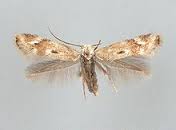
To investigate habitat differences in moth abundances, researchers from the Australian National University (ANU) in Canberra counted the number of individuals of two species of moth (recorded as A and P) along transects throughout a landscape comprising eight different habitat types ('Bank', 'Disturbed', 'Lowerside', 'NEsoak', 'NWsoak', 'SEsoak', 'SWsoak', 'Upperside'). For the data presented here, one of the habitat types ('Bank') has been ommitted as no moths were encounted in that habitat.

Although each transect was approximately the same length, each transect passed through multiple habitat types. Consequently, each transect was divided into sections according to habitat and the number of moths observed in each section recorded. Clearly, the number of observed moths in a section would be related to the length of the transect in that section. Therefore, the researchers also recorded the length of each habitat section.

Download moths data set
Format of moth.csv data files
METERS A P HABITAT
25 9 8 NWsoak
37 3 20 SWsoak
109 7 9 Lowerside
10 0 2 Lowerside
133 9 1 Upperside
26 3 18 Disturbed
METERSThe length of the section of transect
AThe number of moth species A observed in section of transect
PThe number of moth species P observed in section of transect
HABITATCategorical listing of the habitat type within section of transect.
Six-plated barnacle

Open
the day data file.
Show code
> moths <- read.csv('../downloads/data/moths.csv', header=T, strip.white=T)
> head(moths)
  METERS A  P   HABITAT
1     25 9  8    NWsoak
2     37 3 20    SWsoak
3    109 7  9 Lowerside
4     10 0  2 Lowerside
5    133 9  1 Upperside
6     26 3 18 Disturbed

The primary focus of this question will be to investigate the effect of habitat on the abundance of moth species A.

  1. To standardize the moth counts for transect section length, we could convert the counts into densities (by dividing the A by METERS. Create such as variable (DENSITY and explore the usual ANOVA assumptions.
    Show code
    > moths <- within(moths, DENSITY<-A/METERS)
    > boxplot(DENSITY~HABITAT, data=moths)
    
    plot of chunk Q2a_1
  2. Clearly, the there is an issue with normality and homogeneity of variance. Perhaps it would be worth transforming density in an attempt to normalize these data. Given that there are densities of zero, a straight logarithmic transformation would not be appropriate. Alternatives could inlude a square-root transform, a forth-root transform and a log plus 1 transform.
    Show code
    > moths <- within(moths, DENSITY<-A/METERS)
    > boxplot(sqrt(DENSITY)~HABITAT, data=moths)
    
    plot of chunk Q2a_2
    > boxplot((DENSITY)^0.25~HABITAT, data=moths)
    
    plot of chunk Q2a_2
    > boxplot(log(DENSITY+1)~HABITAT, data=moths)
    
    plot of chunk Q2a_2
  3. Arguably, non of the above transformations have improved the data's adherence to the linear modelling assumptions. Count data (such as the abundance of moth species A) is unlikely to follow a normal or even log-normal distribution. Count data are usually more appropriately modelled via a Poisson distribution. Note, dividing by transect length is unlikely to alter the underlying nature of the data distribution as it still based on counts. Fit the generalized linear model (GLM) relating the number of newly recruited barnacles to substrate type. $$log(\mu) = \beta_0+\beta_1 Habitat_i+\epsilon_i, \hspace{1cm} \epsilon \sim Poisson(\lambda)$$
    Show code
    > moths.glm <- glm(A~HABITAT, data=moths, family=poisson)
    
  4. Actually, the above model fails to account for the length of the section of transect. We could do this a couple of ways:
    1. Add METERS as a covariate. Note, since we are modelling against a Poission distribution with a log link function, we should also log the covariate - in order to maintain linearity between the expected value of species A abundance and transect length. $$log(\mu) = \beta_0+\beta_1 Habitat_i + \beta_2 log(meters) +\epsilon_i, \hspace{1cm} \epsilon \sim Poisson(\lambda)$$
      Show code
      > moths.glmC <- glm(A~log(METERS)+HABITAT, data=moths, family=poisson)
      
    2. Add METERS as an offset in which case $\beta_2$ is assumed to be 1 (a reasonable assumption in this case). The advantage is that it does not sacrifice any residual degrees of freedom. Again to maintain linearity, the offset should include the log of transect length. $$log(\mu) = \beta_0+\beta_1 Habitat_i + log(meters) +\epsilon_i, \hspace{1cm} \epsilon \sim Poisson(\lambda)$$
      Show code
      > moths.glmO <- glm(A~HABITAT, offset=log(METERS), data=moths, family=poisson)
      
  5. Check the model for lack of fit via:
    • Pearson Χ2
      Show code
      > moths.resid <- sum(resid(moths.glmO, type="pearson")^2)
      > 1-pchisq(day.resid, moths.glmO$df.resid)
      
      [1] 0.9886
      
      > #No evidence of a lack of fit
      
    • Standardized residuals (plot)
      Show code
      > plot(moths.glmO)
      
      plot of chunk Q2a_5b
      plot of chunk Q2a_5b
      plot of chunk Q2a_5b
      plot of chunk Q2a_5b
      > plot(resid(moths.glmO, type="pearson") ~ fitted(moths.glmO))
      
      plot of chunk Q2a_5b
      > plot(resid(moths.glmO, type="pearson") ~ predict(moths.glmO, type="link"))
      
      plot of chunk Q2a_5b
  6. Estimate the dispersion parameter to evaluate over dispersion in the fitted model
    • Via Pearson residuals
      Show code
      > moths.resid/moths.glmO$df.resid
      
      [1] 8.843
      
      > #No evidence of over dispersion
      
    • Via deviance
      Show code
      > moths.glmO$deviance/moths.glmO$df.resid
      
      [1] 5.463
      
      > #No evidence of over dispersion
      
  7. Compare the expected number of zeros to the actual number of zeros to determine whether the model might be zero inflated.
    • Calculate the proportion of zeros in the data
      Show code
      > moths.tab<-table(moths$A==0)
      > moths.tab/sum(moths.tab)
      
      FALSE  TRUE 
       0.85  0.15 
      
    • Now work out the proportion of zeros we would expect from a Poisson distribution with a lambda equal to the mean count of moths in this study.
      Show code
      > moths.mu <- mean(moths$A)
      > cnts <-rpois(1000,moths.mu)
      > moths.tab<-table(cnts==0)
      > moths.tab/sum(moths.tab)
      
      FALSE  TRUE 
      0.994 0.006 
      
      Clearly there are not more zeros than expected so the data are not zero inflated.

Poisson t-test with overdispersion

The same marine ecologist that featured earlier was also interested in examining the effects of wave exposure on the abundance of another intertidal marine limpet Cellana tramoserica on rocky intertidal shores. Again, a single quadrat was placed on 10 exposed (to large waves) shores and 10 sheltered shores. From each quadrat, the number of smooth limpets (Cellana tramoserica) were counted.

Download LimpetsSmooth data set
Format of limpetsSmooth.csv data files
CountShore
4sheltered
1sheltered
2sheltered
0sheltered
4sheltered
......

ShoreCategorical description of the shore type (sheltered or exposed) - Predictor variable
CountNumber of limpets per quadrat - Response variable
turf

Open the limpetsSmooth data set.

Show code
> limpets <- read.table('../downloads/data/limpetsSmooth.csv', header=T, sep=',', strip.white=T)
> limpets
   Count     Shore
1      3 sheltered
2      1 sheltered
3      6 sheltered
4      0 sheltered
5      4 sheltered
6      3 sheltered
7      8 sheltered
8      1 sheltered
9     13 sheltered
10     0 sheltered
11     2   exposed
12    14   exposed
13     2   exposed
14     3   exposed
15    31   exposed
16     1   exposed
17    13   exposed
18     8   exposed
19    14   exposed
20    11   exposed
  1. We might have initially have been tempted to perform a simple t-test on these data. However, as the response are counts (and close to zero), lets instead fit the same model with a Poisson distribution. $$log(\mu) = \beta_0+\beta1Shore_i+\epsilon_i, \hspace{1cm} \epsilon \sim Poisson(\lambda)$$
    Show code
    > limpets.glm <- glm(Count~Shore, family=poisson, data=limpets)
    
    1. Check the model for lack of fit via:
      • Pearson Χ2
        Show code
        > limpets.resid <- sum(resid(limpets.glm, type="pearson")^2)
        > 1-pchisq(limpets.resid, limpets.glm$df.resid)
        
        [1] 4.441e-16
        
        > #Evidence of a lack of fit
        
      • Deviance (G2)
        Show code
        > 1-pchisq(limpets.glm$deviance, limpets.glm$df.resid)
        
        [1] 1.887e-15
        
        > #Evidence of a lack of fit
        
      • Standardized residuals (plot)
        Show code
        > plot(limpets.glm)
        
        plot of chunk Q31c
        plot of chunk Q31c
        plot of chunk Q31c
        plot of chunk Q31c
    2. Estimate the dispersion parameter to evaluate over dispersion in the fitted model
      • Via Pearson residuals
        Show code
        > limpets.resid/limpets.glm$df.resid
        
        [1] 6.358
        
        > #Evidence of over dispersion
        
      • Via deviance
        Show code
        > limpets.glm$deviance/limpets.glm$df.resid
        
        [1] 6.178
        
        > #Evidence of over dispersion
        
    3. Compare the expected number of zeros to the actual number of zeros to determine whether the model might be zero inflated.
      • Calculate the proportion of zeros in the data
        Show code
        > limpets.tab<-table(limpets$Count==0)
        > limpets.tab/sum(limpets.tab)
        
        FALSE  TRUE 
          0.9   0.1 
        
      • Now work out the proportion of zeros we would expect from a Poisson distribution with a lambda equal to the mean count of limpets in this study.
        Show code
        > limpets.mu <- mean(limpets$Count)
        > cnts <-rpois(1000,limpets.mu)
        > limpets.tab<-table(cnts==0)
        > limpets.tab/sum(limpets.tab)
        
        FALSE  TRUE 
        0.999 0.001 
        
        There is a suggestion that there are more zeros than we should expect given the means of each population. It may be that these data are zero inflated, however, given that our other diagnostics have suggested that the model itself might be inappropriate, zero inflation is not the primary concern.
  2. Clearly there is an issue of with overdispersion. There are multiple potential reasons for this. It could be that there are major sources of variability that are not captured within the sampling design. Alternatively it could be that the data are very clumped. For example, often species abundances are clumped - individuals are either not present, or else when they are present they occur in groups.

  3. As part of the routine exploratory data analysis:
    1. Explore the distribution of counts from each population
      Show code
      > boxplot(Count~Shore,data=limpets)
      > rug(jitter(limpets$Count), side=2)
      
      plot of chunk Q32
      There does appear to be some clumping which might suggest that there are other unmeasured influences.
  4. There are generally two ways of handling this form of overdispersion.
    1. Fit the model with a quasipoisson distribution in which the dispersion factor (lambda) is not assumed to be 1. The degree of variability (and how this differs from the mean) is estimated and the dispersion factor is incorporated.
      Show code
      > limpets.glmQ <- glm(Count~Shore, family=quasipoisson, data=limpets)
      
      1. t-tests
      2. Show code
        > summary(limpets.glmQ)
        
        Call:
        glm(formula = Count ~ Shore, family = quasipoisson, data = limpets)
        
        Deviance Residuals: 
           Min      1Q  Median      3Q     Max  
        -3.635  -2.630  -0.475   1.045   5.345  
        
        Coefficients:
                       Estimate Std. Error t value Pr(>|t|)    
        (Intercept)       2.293      0.253    9.05  4.1e-08 ***
        Shoresheltered   -0.932      0.477   -1.95    0.066 .  
        ---
        Signif. codes:  0 '***' 0.001 '**' 0.01 '*' 0.05 '.' 0.1 ' ' 1
        
        (Dispersion parameter for quasipoisson family taken to be 6.358)
        
            Null deviance: 138.18  on 19  degrees of freedom
        Residual deviance: 111.20  on 18  degrees of freedom
        AIC: NA
        
        Number of Fisher Scoring iterations: 5
        
      3. Wald F-test. Note that F = t2
      4. Show code
        > library(car)
        > Anova(limpets.glmQ,test.statistic="F")
        
        Analysis of Deviance Table (Type II tests)
        
        Response: Count
                   SS Df    F Pr(>F)  
        Shore      27  1 4.24  0.054 .
        Residuals 114 18              
        ---
        Signif. codes:  0 '***' 0.001 '**' 0.01 '*' 0.05 '.' 0.1 ' ' 1
        
        > #OR
        > anova(limpets.glmQ,test="F")
        
        Analysis of Deviance Table
        
        Model: quasipoisson, link: log
        
        Response: Count
        
        Terms added sequentially (first to last)
        
        
              Df Deviance Resid. Df Resid. Dev    F Pr(>F)  
        NULL                     19        138              
        Shore  1       27        18        111 4.24  0.054 .
        ---
        Signif. codes:  0 '***' 0.001 '**' 0.01 '*' 0.05 '.' 0.1 ' ' 1
        
    2. Fit the model with a negative binomial distribution (which accounts for the clumping).
      Show code
      > limpets.glmNB <- glm.nb(Count~Shore, data=limpets)
      
      Check the fit
      Show code
      > limpets.resid <- sum(resid(limpets.glmNB, type="pearson")^2)
      > 1-pchisq(limpets.resid, limpets.glmNB$df.resid)
      
      [1] 0.4334
      
      > #Deviance
      > 1-pchisq(limpets.glmNB$deviance, limpets.glmNB$df.resid)
      
      [1] 0.2155
      
      1. Wald z-tests (these are equivalent to t-tests)
      2. Show code
        > summary(limpets.glmNB)
        
        Call:
        glm.nb(formula = Count ~ Shore, data = limpets, init.theta = 1.283382111, 
            link = log)
        
        Deviance Residuals: 
           Min      1Q  Median      3Q     Max  
        -1.893  -1.093  -0.231   0.394   1.532  
        
        Coefficients:
                       Estimate Std. Error z value Pr(>|z|)    
        (Intercept)       2.293      0.297    7.73  1.1e-14 ***
        Shoresheltered   -0.932      0.438   -2.13    0.033 *  
        ---
        Signif. codes:  0 '***' 0.001 '**' 0.01 '*' 0.05 '.' 0.1 ' ' 1
        
        (Dispersion parameter for Negative Binomial(1.283) family taken to be 1)
        
            Null deviance: 26.843  on 19  degrees of freedom
        Residual deviance: 22.382  on 18  degrees of freedom
        AIC: 122
        
        Number of Fisher Scoring iterations: 1
        
        
                      Theta:  1.283 
                  Std. Err.:  0.506 
        
         2 x log-likelihood:  -116.018 
        
      3. Wald Chisq-test. Note that Chisq = z2
      4. Show code
        > library(car)
        > Anova(limpets.glmNB,test.statistic="Wald")
        
        Analysis of Deviance Table (Type II tests)
        
        Response: Count
                  Df Chisq Pr(>Chisq)  
        Shore      1  4.53      0.033 *
        Residuals 18                   
        ---
        Signif. codes:  0 '***' 0.001 '**' 0.01 '*' 0.05 '.' 0.1 ' ' 1
        
        > anova(limpets.glmNB,test="F")
        
        Analysis of Deviance Table
        
        Model: Negative Binomial(1.283), link: log
        
        Response: Count
        
        Terms added sequentially (first to last)
        
        
              Df Deviance Resid. Df Resid. Dev    F Pr(>F)  
        NULL                     19       26.8              
        Shore  1     4.46        18       22.4 4.46  0.035 *
        ---
        Signif. codes:  0 '***' 0.001 '**' 0.01 '*' 0.05 '.' 0.1 ' ' 1
        
        > anova(limpets.glmNB,test="Chisq")
        
        Analysis of Deviance Table
        
        Model: Negative Binomial(1.283), link: log
        
        Response: Count
        
        Terms added sequentially (first to last)
        
        
              Df Deviance Resid. Df Resid. Dev Pr(>Chi)  
        NULL                     19       26.8           
        Shore  1     4.46        18       22.4    0.035 *
        ---
        Signif. codes:  0 '***' 0.001 '**' 0.01 '*' 0.05 '.' 0.1 ' ' 1
        

Poisson t-test with zero-inflation

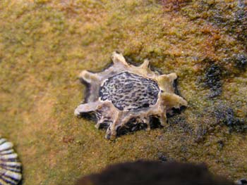
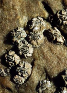
Yet again our rather fixated marine ecologist has returned to the rocky shore with an interest in examining the effects of wave exposure on the abundance of yet another intertidal marine limpet Patelloida latistrigata on rocky intertidal shores. It would appear that either this ecologist is lazy, is satisfied with the methodology or else suffers from some superstition disorder (that prevents them from deviating too far from a series of tasks), and thus, yet again, a single quadrat was placed on 10 exposed (to large waves) shores and 10 sheltered shores. From each quadrat, the number of scaley limpets (Patelloida latistrigata) were counted. Initially, faculty were mildly interested in the research of this ecologist (although lets be honest, most academics usually only display interest in the work of the other members of their school out of politeness - Oh I did not say that did I?). Nevertheless, after years of attending seminars by this ecologist in which the only difference is the target species, faculty have started to display more disturbing levels of animosity towards our ecologist. In fact, only last week, the members of the school's internal ARC review panel (when presented with yet another wave exposure proposal) were rumored to take great pleasure in concocting up numerous bogus applications involving hedgehogs and balloons just so they could rank our ecologist proposal outside of the top 50 prospects and ... Actually, I may just have digressed!

Download LimpetsScaley data set
Format of limpetsScaley.csv data files
CountShore
4sheltered
1sheltered
2sheltered
0sheltered
4sheltered
......

ShoreCategorical description of the shore type (sheltered or exposed) - Predictor variable
CountNumber of limpets per quadrat - Response variable
turf

Open the limpetsSmooth data set.

Show code
> limpets <- read.table('../downloads/data/limpetsScaley.csv', header=T, sep=',', strip.white=T)
> limpets
   Count     Shore
1      2 sheltered
2      1 sheltered
3      3 sheltered
4      1 sheltered
5      0 sheltered
6      0 sheltered
7      1 sheltered
8      0 sheltered
9      2 sheltered
10     1 sheltered
11     4   exposed
12     9   exposed
13     3   exposed
14     1   exposed
15     3   exposed
16     0   exposed
17     0   exposed
18     7   exposed
19     8   exposed
20     5   exposed
  1. As part of the routine exploratory data analysis:
    1. Explore the distribution of counts from each population
      Show code
      > boxplot(Count~Shore,data=limpets)
      > rug(jitter(limpets$Count), side=2)
      
      plot of chunk Q4_1a
    2. Compare the expected number of zeros to the actual number of zeros to determine whether the model might be zero inflated.
      • Calculate the proportion of zeros in the data
        Show code
        > limpets.tab<-table(limpets$Count==0)
        > limpets.tab/sum(limpets.tab)
        
        FALSE  TRUE 
         0.75  0.25 
        
      • Now work out the proportion of zeros we would expect from a Poisson distribution with a lambda equal to the mean count of limpets in this study.
        Show code
        > limpets.mu <- mean(limpets$Count)
        > cnts <-rpois(1000,limpets.mu)
        > limpets.tab<-table(cnts==0)
        > limpets.tab/sum(limpets.tab)
        
        FALSE  TRUE 
         0.91  0.09 
        
        Clearly there are substantially more zeros than expected so the data are likely to be zero inflated.
  2. Lets then fit these data via a zero-inflated Poisson (ZIP) model.
    Show code
    > library(pscl)
    > limpets.zip <- zeroinfl(Count~Shore|1, dist="poisson",data=limpets)
    
    1. Check the model for lack of fit via:
      • Pearson Χ2
        Show code
        > limpets.resid <- sum(resid(limpets.zip, type="pearson")^2)
        > 1-pchisq(limpets.resid, limpets.zip$df.resid)
        
        [1] 0.281
        
        > #No evidence of a lack of fit
        
    2. Estimate the dispersion parameter to evaluate over dispersion in the fitted model
      • Via Pearson residuals
        Show code
        > limpets.resid/limpets.zip$df.resid
        
        [1] 1.169
        
        > #No evidence of over dispersion
        
  3. We can now test the null hypothesis that there is no effect of shore type on the abundance of scaley limpets;
    1. Wald z-tests (these are equivalent to t-tests)
    2. Show code
      > summary(limpets.zip)
      
      Call:
      zeroinfl(formula = Count ~ Shore | 1, data = limpets, dist = "poisson")
      
      Pearson residuals:
         Min     1Q Median     3Q    Max 
      -1.540 -0.940 -0.047  0.846  1.769 
      
      Count model coefficients (poisson with log link):
                     Estimate Std. Error z value Pr(>|z|)    
      (Intercept)       1.600      0.162    9.89  < 2e-16 ***
      Shoresheltered   -1.381      0.362   -3.82  0.00014 ***
      
      Zero-inflation model coefficients (binomial with logit link):
                  Estimate Std. Error z value Pr(>|z|)  
      (Intercept)   -1.700      0.757   -2.25    0.025 *
      ---
      Signif. codes:  0 '***' 0.001 '**' 0.01 '*' 0.05 '.' 0.1 ' ' 1 
      
      Number of iterations in BFGS optimization: 13 
      Log-likelihood: -37.5 on 3 Df
      
    3. Chisq-test. Note that Chisq = z2
    4. Show code
      > library(car)
      > Anova(limpets.zip,test.statistic="Chisq")
      
      Analysis of Deviance Table (Type II tests)
      
      Response: Count
                Df Chisq Pr(>Chisq)    
      Shore      1  14.6    0.00014 ***
      Residuals 17                     
      ---
      Signif. codes:  0 '***' 0.001 '**' 0.01 '*' 0.05 '.' 0.1 ' ' 1
      
    5. F-test. Note that Chisq = z2
    6. Show code
      > library(car)
      > Anova(limpets.zip,test.statistic="F")
      
      Analysis of Deviance Table (Type II tests)
      
      Response: Count
                Df    F Pr(>F)   
      Shore      1 14.6 0.0014 **
      Residuals 17               
      ---
      Signif. codes:  0 '***' 0.001 '**' 0.01 '*' 0.05 '.' 0.1 ' ' 1
      
Interestingly, did you notice that whilst this particular marine ecologists' imagination for design seems somewhat limited, they clearly have a reasonably large statistical tool bag.

Log-linear modelling

Roberts (1993) was intested in examining the interaction between the presence of dead coolibah trees and the position of quadrats along a transect.

Download Roberts data set
Format of roberts.csv data file
COOLIBAHPOSITIONCOUNT
WITHBOTTOM15
WITHMIDDLE4
WITHTOP0
WITHOUTBOTTOM13
WITHOUTMIDDLE8
WITHOUTTOP17

COOLIBAHCategorical listing whether or not dead coolibahs are present (WITH) or absent (WITHOUT) from the quadrat
POSITIONPosition of the quadrat along a transect
PANumber of quadrats in each classification

Coolibah tree

Open the roberts data file (HINT).
Show code
> roberts <- read.table('../downloads/data/roberts.csv', header=T, sep=',', strip.white=T)
> head(roberts)
  COOLIBAH POSITION COUNT
1     WITH   BOTTOM    15
2     WITH   MIDDLE     4
3     WITH      TOP     0
4  WITHOUT   BOTTOM    13
5  WITHOUT   MIDDLE     8
6  WITHOUT      TOP    17
  1. Fit a log-linear model to examine the interaction between presence of dead coolibah trees and position along transect HINT) by first fitting a reduced model (one without the interaction, HINT), then fitting the full model (one with the interaction, HINT) and finally comparing the reduced model to the full model via analysis of deviance (HINT).
    Show code
    > #Reduced model
    > roberts.glmR <- glm(COUNT ~ POSITION + COOLIBAH, family=poisson, data=roberts)
    > #Full model
    > roberts.glmF <- glm(COUNT ~ POSITION * COOLIBAH, family=poisson, data=roberts)
    > #Compare the two models
    > anova(roberts.glmR,roberts.glmF,test='Chisq')
    
    Analysis of Deviance Table
    
    Model 1: COUNT ~ POSITION + COOLIBAH
    Model 2: COUNT ~ POSITION * COOLIBAH
      Resid. Df Resid. Dev Df Deviance Pr(>Chi)    
    1         2       18.6                         
    2         0        0.0  2     18.6  9.1e-05 ***
    ---
    Signif. codes:  0 '***' 0.001 '**' 0.01 '*' 0.05 '.' 0.1 ' ' 1
    
    Alternatively, we can just generate an ANOVA (deviance) table from the full model and ignore the non-interaction terms (HINT).
    Show code
    > anova(roberts.glmF, test="Chisq")
    
    Analysis of Deviance Table
    
    Model: poisson, link: log
    
    Response: COUNT
    
    Terms added sequentially (first to last)
    
    
                      Df Deviance Resid. Df Resid. Dev Pr(>Chi)    
    NULL                                  5       32.0             
    POSITION           2     6.90         3       25.1    0.032 *  
    COOLIBAH           1     6.46         2       18.6    0.011 *  
    POSITION:COOLIBAH  2    18.61         0        0.0  9.1e-05 ***
    ---
    Signif. codes:  0 '***' 0.001 '**' 0.01 '*' 0.05 '.' 0.1 ' ' 1
    
    Identify the following:
    1. G2
    2. df
    3. P value
  2. Perhaps to help provide more insights into the drivers of the significant association between the coolibah mortality and position along the transect, we could explore the odds ratios. Recall that for logit models, the slope terms are expressed on the log odds-ratio scale and thus can be simply translated into odds-ratios. That said, again it is only the interaction terms that are of interest.

    Nevertheless, as one of the observed counts is 0, the slope terms for any interactions involving this cell will be very large (and the exponent likely to be infinite). One possible remedy is to refit the model after adding a small constant (such as 0.5) to all the observed counts and then calculate the odds ratios.

    Show code
    > roberts.glmF1 <- glm(I(COUNT+0.5) ~ POSITION*COOLIBAH, family=poisson, data=roberts)
    > library(biology)
    
    Error: there is no package called 'biology'
    
    > odds.ratio(roberts.glmF1)
    
    Error: could not find function "odds.ratio"
    

    An additional issue that no doubt you noticed is that as the model is fitted as an 'effects' parameterization, not all pairwise calculations are defined. For example, the interaction terms define the (log) odds ratios for with and without coolibah trees in the bottom of the transect versus the middle and versus the top. Hence we only have odds ratios for two of the three comparisons (we don't have middle vs top)

    We could derive this other odds ratio by either redefining the model contrasts. Alternatively, we could just calculate the pairwise odds ratios from a cross table representation of the frequency data (again adding a constant of 0.5).

    Show code
    > roberts.xtab <- xtabs(COUNT+0.5~POSITION+COOLIBAH, data=roberts)
    > library(biology)
    
    Error: there is no package called 'biology'
    
    > oddsratios(roberts.xtab)
    
    Error: could not find function "oddsratios"
    
    > #you are 40 times more likely to encounter dead coolibah trees at the bottom of the transect than at the top.
    

    What addition conclusions would you draw?

Log-linear modelling

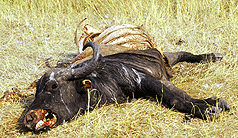
Sinclair investigated the association between sex, health and cause of death in wildebeest. To do so, they recorded the sex and cause of death (predator or not) of wildebeest carcasses along with a classification of a bone marrow sample. The color and consistency of bone marrow is apparently a reasonably good indication of the health status of an animal (even after death).

Download Sinclair data set
Format of sinclair.csv data file
SEXMARROWDEATHCOUNT
FEMALESWFPRED26
MALESWFPRED14
FEMALEOGPRED32
MALEOGPRED43
FEMALETGPRED8
MALETGPRED10
FEMALESWFNPRED6
MALESWFNPRED7
FEMALEOGNPRED26
MALEOGNPRED12
FEMALETGNPRED16
MALETGNPRED26

Wildebeast carcass
SEXCategorical listing sex of the wildebeast carcasses
MARROWCategorical listing of the bone marrow type (SWF: solid white fatty, OG: opaque gelatinous, TG: translucent gelatinous).
DEATHCategorical listing of the cause of death (predation or non-predation)
COUNTNumber of carcasses encountered in each cross-classification.

Open the sinclair data file (HINT).
Show code
> sinclair <- read.table('../downloads/data/sinclair.csv', header=T, sep=',', strip.white=T)
> head(sinclair)
     SEX MARROW DEATH COUNT
1 FEMALE    SWF  PRED    26
2   MALE    SWF  PRED    14
3 FEMALE     OG  PRED    32
4   MALE     OG  PRED    43
5 FEMALE     TG  PRED     8
6   MALE     TG  PRED    10
  1. What is the null hypothesis of interest?
  2. Log-linear models for three way tables have a greater number of interactions and therefore a greater number of combinations of terms that should be tested. As with ANOVA, it is the higher level interactions (three way) interaction that is of initial interest, followed by the various two way interactions.
  3. Test the null hypothesis that there is no three way interaction (the cause of death is independent of sex and bone marrow type). First fit a reduced model (one that contains all two way interactions as well as individual effects but without the three way interaction, HINT), then fitting the full model (one with the interaction and all other terms, HINT) and finally comparing the reduced model to the full model (HINT).
    Show code
    > sinclair.glmR <- glm(COUNT~SEX:DEATH + SEX:MARROW + MARROW:DEATH + SEX + DEATH + MARROW, family=poisson,data=sinclair)
    > sinclair.glmF <- glm(COUNT~SEX*DEATH*MARROW, family=poisson,data=sinclair)
    > anova(sinclair.glmR,sinclair.glmF,test='Chisq')
    
    Analysis of Deviance Table
    
    Model 1: COUNT ~ SEX:DEATH + SEX:MARROW + MARROW:DEATH + SEX + DEATH + 
        MARROW
    Model 2: COUNT ~ SEX * DEATH * MARROW
      Resid. Df Resid. Dev Df Deviance Pr(>Chi)  
    1         2       7.19                       
    2         0       0.00  2     7.19    0.027 *
    ---
    Signif. codes:  0 '***' 0.001 '**' 0.01 '*' 0.05 '.' 0.1 ' ' 1
    
    > #OR just 
    > anova(sinclair.glmF,test='Chisq')
    
    Analysis of Deviance Table
    
    Model: poisson, link: log
    
    Response: COUNT
    
    Terms added sequentially (first to last)
    
    
                     Df Deviance Resid. Df Resid. Dev Pr(>Chi)    
    NULL                                11       77.0             
    SEX               1     0.02        10       76.9   0.8942    
    DEATH             1     7.12         9       69.8   0.0076 ** 
    MARROW            2    27.05         7       42.8  1.3e-06 ***
    SEX:DEATH         1     0.09         6       42.7   0.7685    
    SEX:MARROW        2     4.78         4       37.9   0.0917 .  
    DEATH:MARROW      2    30.71         2        7.2  2.1e-07 ***
    SEX:DEATH:MARROW  2     7.19         0        0.0   0.0275 *  
    ---
    Signif. codes:  0 '***' 0.001 '**' 0.01 '*' 0.05 '.' 0.1 ' ' 1
    
     G2dfP
    SEX:MARROW:DEATH
  4. We would clearly reject the null hypothesis of no three way interaction. As with ANOVA, following a significant interaction it is necessary to slip the data up according to the levels of one of the factors and explore the patterns further within the multiple subsets.
    1. Sinclair and Arcese (1995) might have been interesting in investigating the associations between cause of death and marrow type separately for each sex. Split the sinclair data set up by sex. (HINT)
    2. Show code
      > sinclair.split <- split(sinclair, sinclair$SEX)
      > sinclair.split
      
      $FEMALE
            SEX MARROW DEATH COUNT
      1  FEMALE    SWF  PRED    26
      3  FEMALE     OG  PRED    32
      5  FEMALE     TG  PRED     8
      7  FEMALE    SWF NPRED     6
      9  FEMALE     OG NPRED    26
      11 FEMALE     TG NPRED    16
      
      $MALE
          SEX MARROW DEATH COUNT
      2  MALE    SWF  PRED    14
      4  MALE     OG  PRED    43
      6  MALE     TG  PRED    10
      8  MALE    SWF NPRED     7
      10 MALE     OG NPRED    12
      12 MALE     TG NPRED    26
      
    3. Perform the log-linear modelling for the associations between cause of death and marrow type separately for each sex.
      Show code
      > sinclair.glmR <- glm(COUNT~DEATH+MARROW, family=poisson, data=sinclair.split[["FEMALE"]])
      > sinclair.glmF <- glm(COUNT~DEATH*MARROW, family=poisson, data=sinclair.split[["FEMALE"]])
      > anova(sinclair.glmR, sinclair.glmF, test="Chisq")
      
      Analysis of Deviance Table
      
      Model 1: COUNT ~ DEATH + MARROW
      Model 2: COUNT ~ DEATH * MARROW
        Resid. Df Resid. Dev Df Deviance Pr(>Chi)    
      1         2         14                         
      2         0          0  2       14  0.00093 ***
      ---
      Signif. codes:  0 '***' 0.001 '**' 0.01 '*' 0.05 '.' 0.1 ' ' 1
      
      > #Alternatively, the splitting and subsetting can be performed inline
      > #I shall illustrate this with the MALE data
      > sinclair.glmR <- glm(COUNT~DEATH+MARROW, family=poisson, data=sinclair, subset=sinclair$SEX=="MALE")
      > sinclair.glmF <- glm(COUNT~DEATH*MARROW, family=poisson, data=sinclair, subset=sinclair$SEX=="MALE")
      > anova(sinclair.glmR, sinclair.glmF, test="Chisq")
      
      Analysis of Deviance Table
      
      Model 1: COUNT ~ DEATH + MARROW
      Model 2: COUNT ~ DEATH * MARROW
        Resid. Df Resid. Dev Df Deviance Pr(>Chi)    
      1         2       23.9                         
      2         0        0.0  2     23.9  6.3e-06 ***
      ---
      Signif. codes:  0 '***' 0.001 '**' 0.01 '*' 0.05 '.' 0.1 ' ' 1
      
    4.  G2dfP
      Females - MARROW:DEATH
      Males - MARROW:DEATH
  5. It appears that there are significant interactions between cause of death and bone marrow type for both females and males. Given that there was a significant interaction between cause of death and sex and bone marrow type, it is likely that the nature of the two way interactions in females is different to the two way interactions in males. To explore this further, we will examine the odds ratios for each pairwise comparison of bone marrow type with respect to predation level (for each sex)!.
    Calculate the odds ratios for wildebeest killed by predation for each pair of marrow types separately for males and females
    .
    Show code
    > library(epitools)
    
    Error: there is no package called 'epitools'
    
    > library(biology)
    
    Error: there is no package called 'biology'
    
    > #Females
    > female.tab <- xtabs(COUNT ~ DEATH + MARROW, data=sinclair.split[["FEMALE"]])
    > female.odds<-oddsratios(t(female.tab))
    
    Error: could not find function "oddsratios"
    
    > female.odds
    
    Error: object 'female.odds' not found
    
    > #Males
    > male.tab <- xtabs(COUNT ~ DEATH + MARROW, data=sinclair.split[["MALE"]])
    > male.odds<-oddsratios(t(male.tab))
    
    Error: could not find function "oddsratios"
    
     Odds ratio95% CI min95% CI max
    Females      
    OG vs TG
    SWF vs TG
    SWF vs OG
    Males      
    OG vs TG
    SWF vs TG
    SWF vs OG
  6. The patterns revealed in the odds ratios might be easier to see, if they were presented graphically - do it.
    Show code
    > par(mar=c(5,5,0,0))
    > plot(estimate~as.numeric(Comparison), data=female.odds, log="y", type="n", axes=F, ann=F, ylim=range(c(upper,lower)), xlim=c(0.5,3.5))
    
    Error: object 'female.odds' not found
    
    > with(female.odds,arrows(as.numeric(Comparison)+0.1,upper,as.numeric(Comparison)+0.1,lower,ang=90,length=0.1,code=3))
    
    Error: object 'female.odds' not found
    
    > with(female.odds,points(as.numeric(Comparison)+0.1,estimate, type="b", pch=21, bg="white"))
    
    Error: object 'female.odds' not found
    
    > #males
    > with(male.odds,arrows(as.numeric(Comparison)-0.1,upper,as.numeric(Comparison)-0.1,lower,ang=90,length=0.1,code=3))
    
    Error: object 'male.odds' not found
    
    > with(male.odds,points(as.numeric(Comparison)-0.1,estimate, type="b", pch=21, bg="black",lty=1))
    
    Error: object 'male.odds' not found
    
    > abline(h=1,lty=2)
    
    Error: plot.new has not been called yet
    
    > with(female.odds, axis(1,at=as.numeric(Comparison), lab=Comparison))
    
    Error: object 'female.odds' not found
    
    > mtext("Marrow type",1,line=3, cex=1.25)
    
    Error: plot.new has not been called yet
    
    > axis(2,las=1)
    
    Error: plot.new has not been called yet
    
    > mtext("Odds ratio of death by predation",2,line=4, cex=1.25)
    
    Error: plot.new has not been called yet
    
    > legend("topright",legend=c("Male","Female"),pch=21, bty="n", title="Sex",pt.bg=c("black","white"))
    
    Error: plot.new has not been called yet
    
    > box(bty="l")
    
    Error: plot.new has not been called yet
    
  7. What would your conclusions be?

  Reading data into R

Ensure that the working directory is pointing to the path containing the file to be imported before proceeding.
To import data into R, we read the contents of a file into a data frame. The general format of the command for reading data into a data frame is

> name <- read.table('filename.csv', header=T, sep=',', row.names=column, strip.white=T)

where name is a name you wish the data frame to be referred to as, filename.csv is the name of the csv file that you created in excel and column is the number of the column that had row labels (if there were any). The argument header=T indicates that the variable (vector) names will be created from the names supplied in the first row of the file. The argument sep=',' indicates that entries in the file are separated by a comma (hence a comma delimited file). If the data file does not contain row labels, or you are not sure whether it does, it is best to omit the row.names=column argument. The strip.white=T arguement ensures that no leading or trailing spaces are left in character names (these can be particularly nasty in categorical variables!).

As an example
> phasmid <- read.data('phasmid.csv', header=T, sep=',', row.names=1, strip.white=T)

End of instructions