Tutorial 10.3a - Contingency tables
22 Jul 2018
Scenario and Data
Contingency tables are concerned with exploring associations between two or three cross-classified factors. In essence, a table of observed frequencies (number of observations in each classification combination - table cell) are compared to the frequencies expected under some null hypothesis (no association). Lets say for example we had cross-classified a number of items into one of two levels of A (a1 and a2) and one of three levels of B (b1, b2 and b3).
| Factor B | ||||
|---|---|---|---|---|
| b1 | b2 | b3 | ||
| Factor A | a1 | a1b1 | a1b2 | a1b3 |
| a2 | a2b1 | a2b2 | a2b3 |
Lets now generate some artificial. As this section is mainly about the generation of artificial data (and not specifically about what to do with the data), understanding the actual details are optional and can be safely skipped. Consequently, I have folded (toggled) this section away.
- the base frequency (counts) are approximately 20 (a random number drawn from a Poisson distribution with centrality parameter of 20).
- the "effect" of a2 (difference in counts between a2 and a1 at level b1) is approximately 10
- the "effect" of b2 (difference in counts between b2 and b1 at level a1) is approximately -5
- the "effect" of b3 (difference in counts between b3 and b1 at level a1) is approximately -10
- the interaction "effect" of a2b2 (difference between a2b2 and a1b1 plus a2 effect plus b2 effect) is approximately 20
- the interaction "effect" of a2b3 (difference between a2b3 and a1b1 plus a2 effect plus b3 effect) is approximately -10
set.seed(4)
base <- rpois(1, 20)  # (a1b1~ 20)
base
[1] 20
# Effect of a2 vs a1 (at b1) ~ 10
a2eff <- rpois(1, 10)  # (a2b1~30)
a2eff
[1] 8
# Effect of b2 vs b1 (at a1) ~ -5
b2eff <- -1 * rpois(1, 5)  # (a1b2=15)
b2eff
[1] -7
# Effect of b3 vs b1 (at a1) ~ -10
b3eff <- -1 * rpois(1, 10)  # (a1b3=5)
b3eff
[1] -7
# Interaction effects Effect of a2b2 vs a2b1 ~ 20
a2b2eff <- rpois(1, 20)
a2b2eff
[1] 27
# Effect of a2b3 vs a2b1 ~ -10
a2b3eff <- -1 * rpois(1, 10)
a2b3eff
[1] -12
# Create the cross-classification factors as a data frame
dat <- expand.grid(A = c("a1", "a2"), B = c("b1", "b2", "b3"))
# Create an effects model matrix
dat.mm <- model.matrix(~A * B, dat)
# Calculate the outer product of the effects model matrix and the effects parameters
dat$Counts <- dat.mm %*% c(base, a2eff, b2eff, b3eff, a2b2eff, a2b3eff)
# View the resulting data
dat
   A  B Counts
1 a1 b1     20
2 a2 b1     28
3 a1 b2     13
4 a2 b2     48
5 a1 b3     13
6 a2 b3      9
| Factor B | ||||
|---|---|---|---|---|
| b1 | b2 | b3 | ||
| Factor A | a1 | 20 | 13 | 13 |
| a2 | 28 | 48 | 9 |
With these sort of data, we are primarily interested in investigating whether there is an association between Factor A and Factor B. By association, we mean interaction. That is, are the differences in counts between each level of A (a1 and a2) consistent across all levels of Factor B (b1, b2 and b3)? One of the ways of exploring this is with a $\chi^2$ statistic. The $\chi^2$ statistic compares an observed ($o$) frequencies to those expected ($e$) when the null hypothesis (no association between the Factors) is true. $$\chi^2=\sum\frac{(o-e)^2}{e}$$
When the null hypothesis is true, and specific assumptions hold, the $\chi^2$ statistic should follow a $\chi^2$ probability distribution with degrees of freedom equal to the ($df=({number~of~rows-1})\times({number~of~colummns-1})$).
Exploratory data analysis and initial assumption checking
- All of the observations are classified independently - this must be addressed at the design and collection stages
- No more than 20% of the expected values should be less than 5. Since the location and spread of the expected value of a $\chi^2$ distribution are the same parameter ($\lambda$), and that the $\chi^2$ distribution is bounded by a lower limit of zero, distributions with expected values less than 5 have an asymmetrical shape and are thus unreliable (for calculating probabilities).
So lets calculate the expected frequencies as a means to evaluate this assumption. The expected values within any cell of the table are calculated as: $$e = \frac{({row~total}\times{column~total})}{{grand~total}}$$
| Factor B | |||||
|---|---|---|---|---|---|
| b1 | b2 | b3 | Total | ||
| Factor A | a1 | e=(a1tot*b1tot)/tot | e=(a1tot*b2tot)/tot | e=(a1tot*b3tot)/tot | a1tot=a1b1+a1b2+a1b3 |
| a2 | e=(a2tot*b1tot)/tot | e=(a2tot*b2tot)/tot | e=(a2tot*b3tot)/tot | a2tot=a2b1+a2b2+a2b3 | |
| Total | b1tot=a1b1+a2b1 | b2tot=a1b2+a2b2 | b2tot=a1b3+a2b3 | tot=a1tot+a2tot |
We can use matrix algebra to calculate the expected counts (based on the scheme outlined above). What we want to do is calculate the outer product of the row totals and the column totals and then divide the outer product by the grand total. This can be visualized as: $$e_i = \frac{ \begin{bmatrix} a1total\\a2total \end{bmatrix}\times \begin{bmatrix} b1total, b2total, b3total \end{bmatrix} }{Grand total} $$ In order to perform this in R, we first need to convert the data into a cross-table (a special type of matrix). This is achieved via the xtabs function. In R, the rowSums and colSums functions can be used to calculate the row and column sums of a matrix respectively. The %o% function (actually an operator in disguise) is used to calculate the outer product of two arrays or matrices.
dat.xtab <- xtabs(Counts ~ A + B, dat)
(rowSums(dat.xtab) %o% colSums(dat.xtab))/sum(dat.xtab)
         b1       b2        b3
a1 16.85496 21.41985  7.725191
a2 31.14504 39.58015 14.274809
As the expected values are all greater than 5, the $\chi^2$ statistic is likely to be reliable.
Model fitting or statistical analysis
We perform the contingency table $\chi^2$ test with the chisq.test() function. There are only two relevant parameters for a contingency table chi-square test:
- x: the cross table of observed frequencies
- correct: whether or not to perform Yates' corrections for small sample sizes. These are no longer considered all that appropriate. Indeed there are far more appropriate means of dealing with small samples sizes (notably log-linear modelling).
dat.chisq <- chisq.test(dat.xtab, correct = FALSE)
Model evaluation
Prior to exploring the model parameters, it is prudent to confirm that the model did indeed fit the assumptions and was an appropriate fit to the data. For the $\chi^2$ test, this just means confirming the expected values.
dat.chisq$exp
    B
A          b1       b2        b3
  a1 16.85496 21.41985  7.725191
  a2 31.14504 39.58015 14.274809
Exploring the model parameters, test hypotheses
If there was any evidence that the assumptions had been violated or the model was not an appropriate fit, then we would need to reconsider the model and start the process again. In this case, there is no evidence that the test will be unreliable so we can proceed to explore the test statistics.
dat.chisq
	Pearson's Chi-squared test

data:  dat.xtab
X-squared = 11.556, df = 2, p-value = 0.003095
Conclusions: there is inferential evidence to reject the null hypothesis of no association between Factor A and Factor B. When the null hypothesis is true (no association), we would have expected a $\chi^2$ statistic of approximately 1. The $\chi^2$ statistic resulting from our observed data is substantially (significantly) greater than 1 (11. 56). The probability of obtaining a $\chi^2$ value of 11.56 or greater when the null hypothesis is true is 0.003.
Further explorations of the trends
When a significant association is identified, it is often useful to explore the patterns of residuals. Since the residuals are a (standardized) measure of the differences between observed and expected for each cross-classification group (cells of the table), they provide an indication of which cells deviate most from the expected and therefore which levels of the factors are the main driver(s) of the "effect".
In interpreting the residuals, we are looking for large (substantially larger in magnitude than 1)positive and negative values, which represent higher and lower observed frequencies than would have been expected under the null hypothesis respectively.
dat.chisq$res
    B
A            b1         b2         b3
  a1  0.7660587 -1.8192653  1.8978074
  a2 -0.5635487  1.3383370 -1.3961163
Conclusions: there were fewer observations classified as b3 and more classified as b3 when Factor A is a1 and the reverse when Factor A is a2 than would have been expected. Hence Factor B levels b2 and b3 are the main drivers of the association between Factor A and Factor B
Another useful measure is the odds-ratios. Odds ratios are a measure of the relative odds (probabilities) of events under different scenarios. In this case, we could calculate the odds ratios of a1 vs a2 for each pair of Factor B levels. Odds that deviate substantially from 1 are indicative
library(biology)
Error in library(biology): there is no package called 'biology'
# We perform pairwise oddsratios on the transposed cross table
oddsratios(t(dat.xtab))
Error in eval(expr, envir, enclos): could not find function "oddsratios"
We could even plot the odds ratios.
library(biology)
Error in library(biology): there is no package called 'biology'
        #Create an empty object in which to store the odds ratios
        or <- NULL
        #Get the colnames from the cross table
        nms <- colnames(dat.xtab)
        #Calculate each pairwise odds ratio
        for (i in 1:ncol(dat.xtab)) {
        for (j in 1:ncol(dat.xtab)) {
        if (i == j) next
        or <- rbind(or, cbind(Comp1 = nms[i], Comp2 = nms[j], oddsratios(dat.xtab[, c(i, j)])))
        }
        }
Error in cbind(Comp1 = nms[i], Comp2 = nms[j], oddsratios(dat.xtab[, c(i, : could not find function "oddsratios"
        or$Comp2s <- as.numeric(factor(as.character(or$Comp2)))
        opar <- par(mar = c(5, 6, 1, 1))
        plot(estimate ~ Comp2s, data = or, axes = F, ann = F, type = "n", log = "y",
        ylim = c(min(or$lower), max(or$upper)), xlim = c(0, 4))
Error in eval(expr, envir, enclos): object 'estimate' not found
abline(h = 1, lty = 2)
Error in int_abline(a = a, b = b, h = h, v = v, untf = untf, ...): plot.new has not been called yet
with(subset(or, Comp1 == "b1"), arrows(Comp2s - 0.1,lower,Comp2s-0.1,upper,code = 3,length = 0.05,ang = 90))
Error in subset.default(or, Comp1 == "b1"): object 'Comp1' not found
points(estimate ~ I(Comp2s - 0.1), data = subset(or, Comp1 == "b1"), type = "p", pch = 22, bg = "white")
Error in subset.default(or, Comp1 == "b1"): object 'Comp1' not found
with(subset(or, Comp1 == "b2"), arrows(Comp2s - 0,lower,Comp2s -0,upper,code = 3,length = 0.05,ang = 90))
Error in subset.default(or, Comp1 == "b2"): object 'Comp1' not found
points(estimate ~ I(Comp2s - 0), data = subset(or, Comp1 == "b2"), type = "p", pch = 21, bg = "grey70")
Error in subset.default(or, Comp1 == "b2"): object 'Comp1' not found
with(subset(or, Comp1 == "b3"), arrows(Comp2s+0.1,lower,Comp2s+0.1,upper,code = 3,length = 0.05,ang = 90))
Error in subset.default(or, Comp1 == "b3"): object 'Comp1' not found
points(estimate ~ I(Comp2s + 0.1), data = subset(or, Comp1 == "b3"), type = "p", pch = 21, bg = "black")
Error in subset.default(or, Comp1 == "b3"): object 'Comp1' not found
axis(1, at = 1:3, labels = nms)
Error in axis(1, at = 1:3, labels = nms): plot.new has not been called yet
axis(2, las = 1)
Error in axis(2, las = 1): plot.new has not been called yet
mtext("Factor B", 1, line = 3, cex = 1.5)
Error in mtext("Factor B", 1, line = 3, cex = 1.5): plot.new has not been called yet
mtext("Odds ratio", 2, line = 3.5, cex = 1.5)
Error in mtext("Odds ratio", 2, line = 3.5, cex = 1.5): plot.new has not been called yet
legend("topleft", legend = nms, pch = c(22, 21, 21), pt.bg = c("white", "grey70", "black"), bty = "n")
Error in strwidth(legend, units = "user", cex = cex, font = text.font): plot.new has not been called yet
box(bty = "l")
Error in box(bty = "l"): plot.new has not been called yet
Worked Examples
Basic χ2 references
- Logan (2010) - Chpt 16-17
- Quinn & Keough (2002) - Chpt 13-14
Continguency tables
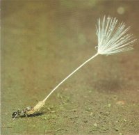
Here is a modified example from Quinn and Keough (2002). Following fire, French and Westoby (1996) cross-classified plant species by two variables: whether they regenerated by seed only or vegetatively and whether they were dispersed by ant or vertebrate vector. The two variables could not be distinguished as response or predictor since regeneration mechanisms could just as conceivably affect dispersal mode as vice versa.
Download French data set| Format of french.csv data files | ||||||||||||||||||||||||||||||||||
|---|---|---|---|---|---|---|---|---|---|---|---|---|---|---|---|---|---|---|---|---|---|---|---|---|---|---|---|---|---|---|---|---|---|---|
|
 |
|||||||||||||||||||||||||||||||||
Open the french data file. HINT.
french <- read.table("../downloads/data/french.csv", header = T, sep = ",", strip.white = T)
head(french)
  regen disp count
1  seed  ant    25
2  seed vert     6
3   veg  ant    36
4   veg vert    21
-
What null hypothesis is being tested by this test?
-
Generate a
cross table
out of the dataset in preparation for frequency analysis (HINT).
Show codefrench.tab <- xtabs(count ~ regen + disp, data = french) french.tab
      disp
regen  ant vert
  seed  25    6
  veg   36   21
- Fit
a 2 x 2 (two way) contingency table
(HINT), and explore the main assumption of the test by examining the expected frequencies
(HINT).
Show code
french.x2 <- chisq.test(french.tab, correct = F)
french.x2$exp
      disp
regen       ant      vert
  seed 21.48864  9.511364
  veg  39.51136 17.488636
-
If the assumption is OK, test this null hypothesis and identify the following.
Show codefrench.x2Pearson's Chi-squared test data: french.tab X-squared = 2.8872, df = 1, p-value = 0.08929
- X2 statistic
- df
- P value
- X2 statistic
- Calculate the odds ratio (odds of vegetative dispersal over seed dispersal for vertebrate dispersed vs ant dispersed)
Show code
library(epitools)
Error in library(epitools): there is no package called 'epitools'
oddsratio(french.tab)
Error in eval(expr, envir, enclos): could not find function "oddsratio"
- What are your conclusions (statistical and biological)?
Contingency table
Arrington et al. (2002) examined the frequency with which African, Neotropical and North American fishes have empty stomachs and found that the mean percentage of empty stomachs was around 16.2%. As part of the investigation they were interested in whether the frequency of empty stomachs was related to dietary items. The data were separated into four major trophic classifications (detritivores, omnivores, invertivores, and piscivores) and whether the fish species had greater or less than 16.2% of individuals with empty stomachs. The number of fish species in each category combination was calculated and a subset of that (just the diurnal fish) is provided.
Download Arrington data set| Format of arrington.csv data file | |||||||||||||||||||||||||||||||||||||||||
|---|---|---|---|---|---|---|---|---|---|---|---|---|---|---|---|---|---|---|---|---|---|---|---|---|---|---|---|---|---|---|---|---|---|---|---|---|---|---|---|---|---|
|

|
||||||||||||||||||||||||||||||||||||||||
arrington <- read.table("../downloads/data/arrington.csv", header = T, sep = ",", strip.white = T)
head(arrington)
  STOMACH TROPHIC
1   <16.2     DET
2   <16.2     DET
3   <16.2     DET
4   <16.2     DET
5   <16.2     DET
6   <16.2     DET
Note the format of the data file. Rather than including a compilation of the observed counts, this data file lists the categories for each individual. This example will demonstrate how to analyse two-way contingency tables from such data files. Each row of the data set represents a separate species of fish that is then cross categorised according to whether the proportion of individuals of that species with empty stomachs was higher or lower than the overall average (16.2%) and to what trophic group they belonged.
- Generate a cross table
out of the raw data file in preparation for the contingency table (HINT).
Show code
arrington.tab <- table(arrington)
arrington.tab
       TROPHIC
STOMACH DET INV OMN PISC
  <16.2  18  58  45   16
  >16.2   4  15   8   34
- Fit the model
(HINT), test the assumptions
(HINT) and, using a
two-way contingency table,
test the null hypothesis that the percentage of empty stomachs was independent of trophic classification
(HINT).
What would you conclude form the analysis?
Show codearrington.x2 <- chisq.test(arrington.tab) arrington.x2$exp
       TROPHIC
STOMACH       DET     INV      OMN     PISC
  <16.2 15.222222 50.5101 36.67172 34.59596
  >16.2  6.777778 22.4899 16.32828 15.40404
arrington.x2Pearson's Chi-squared test data: arrington.tab X-squared = 43.835, df = 3, p-value = 1.636e-09
-
Write the results out as though you were writing a research paper/thesis. For example (select the phrase that applies and fill in gaps with your results):
The percentage of empty stomachs was (choose the correct option)
trophic classification. (X2 =
, df =
, P =
).
-
Generate the residuals
(HINT) associated with the above contingency test and complete the following table of standardized residuals.
Show codearrington.x2$res
       TROPHIC
STOMACH        DET        INV        OMN       PISC
  <16.2  0.7119647  1.0538695  1.3752759 -3.1615926
  >16.2 -1.0669740 -1.5793639 -2.0610342  4.7380678
< 16.2% > 16.2% DET OMN INV PISC - Calculate the odds ratios for the different trophic levels
Show code
library(biology)
Error in library(biology): there is no package called 'biology'
or <- NULL
nms <- colnames(arrington.tab)
for (i in 1:ncol(arrington.tab)) {
    for (j in 1:ncol(arrington.tab)) {
        if (i == j)
            next
        or <- rbind(or, cbind(Comp1 = nms[i], Comp2 = nms[j], oddsratios(arrington.tab[, c(i, j)])))
    }
}
Error in cbind(Comp1 = nms[i], Comp2 = nms[j], oddsratios(arrington.tab[, : could not find function "oddsratios"
or$Comp2s <- as.numeric(factor(as.character(or$Comp2)))
opar <- par(mar = c(5, 6, 1, 1))
plot(estimate ~ Comp2s, data = or, axes = F, ann = F, type = "n", log = "y", ylim = c(min(lower), max(upper)),
    xlim = c(0, 5))
Error in eval(expr, envir, enclos): object 'lower' not found
abline(h = 1, lty = 2)
Error in int_abline(a = a, b = b, h = h, v = v, untf = untf, ...): plot.new has not been called yet
with(subset(or, Comp1 == "DET"), arrows(Comp2s - 0.1, lower, Comp2s - 0.1, upper, code = 3, length = 0.1,
    ang = 90))
Error in subset.default(or, Comp1 == "DET"): object 'Comp1' not found
points(estimate ~ I(Comp2s - 0.1), data = subset(or, Comp1 == "DET"), type = "p", pch = 22, bg = "white")
Error in subset.default(or, Comp1 == "DET"): object 'Comp1' not found
with(subset(or, Comp1 == "INV"), arrows(Comp2s - 0.05, lower, Comp2s - 0.05, upper, code = 3, length = 0.1,
    ang = 90))
Error in subset.default(or, Comp1 == "INV"): object 'Comp1' not found
points(estimate ~ I(Comp2s - 0.05), data = subset(or, Comp1 == "INV"), type = "p", pch = 21, bg = "grey90")
Error in subset.default(or, Comp1 == "INV"): object 'Comp1' not found
with(subset(or, Comp1 == "OMN"), arrows(Comp2s + 0.05, lower, Comp2s + 0.05, upper, code = 3, length = 0.1,
    ang = 90))
Error in subset.default(or, Comp1 == "OMN"): object 'Comp1' not found
points(estimate ~ I(Comp2s + 0.05), data = subset(or, Comp1 == "OMN"), type = "p", pch = 21, bg = "grey50")
Error in subset.default(or, Comp1 == "OMN"): object 'Comp1' not found
with(subset(or, Comp1 == "PISC"), arrows(Comp2s + 0.1, lower, Comp2s + 0.1, upper, code = 3, length = 0.1,
    ang = 90))
Error in subset.default(or, Comp1 == "PISC"): object 'Comp1' not found
points(estimate ~ I(Comp2s + 0.1), data = subset(or, Comp1 == "PISC"), type = "p", pch = 21, bg = "black")
Error in subset.default(or, Comp1 == "PISC"): object 'Comp1' not found
axis(1, at = 1:4, labels = nms)
Error in axis(1, at = 1:4, labels = nms): plot.new has not been called yet
axis(2, las = 1)
Error in axis(2, las = 1): plot.new has not been called yet
mtext("Trophic level", 1, line = 3, cex = 1.5)
Error in mtext("Trophic level", 1, line = 3, cex = 1.5): plot.new has not been called yetmtext("Odds ratio of empty stomachs by trophic level", 2, line = 3.5, cex = 1.5)
Error in mtext("Odds ratio of empty stomachs by trophic level", 2, line = 3.5, : plot.new has not been called yetlegend("topleft", legend = nms, pch = c(22, 21, 21, 21), pt.bg = c("white", "grey90", "grey50", "black"), bty = "n")
Error in strwidth(legend, units = "user", cex = cex, font = text.font): plot.new has not been called yet
box(bty = "l")
Error in box(bty = "l"): plot.new has not been called yet
par(opar)
- What further conclusions would you draw from the standardized residuals?
Contingency tables
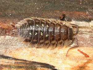
Here is an example (13.5) from Fowler, Cohen and Parvis (1998). A field biologist collected leaf litter from a 1 m2 quadrats randomly located on the ground at night in two locations - one was on clay soil the other on chalk soil. The number of woodlice of two different species (Oniscus and Armadilidium) were collected and it is assumed that all woodlice undertake their nocturnal activities independently. The number of woodlice are in the following contingency table.
Download Woodlice data set| Format of Woodlice data set | |||||||||||||
|---|---|---|---|---|---|---|---|---|---|---|---|---|---|
|
 |
||||||||||||
woodlice <- read.table("../downloads/data/woodlice.csv", header = T, sep = ",", strip.white = T)
head(woodlice)
   SOIL      SPECIES COUNTS
1  Clay      oniscus     14
2  Clay armadilidium      6
3 Chalk      oniscus     22
4 Chalk armadilidium     46
- What null hypothesis is being tested by this test?
- Generate a
cross table
out of the dataset in preparation for frequency analysis
(HINT).
Show codewoodlice.tab <- xtabs(COUNTS ~ SOIL + SPECIES, data = woodlice) woodlice.tab
       SPECIES
SOIL    armadilidium oniscus
  Chalk           46      22
  Clay             6      14
- Fit
a 2 x 2 (two way) contingency table
(HINT),
and explore the main assumption of the test by examining the expected frequencies (HINT).
Show code
woodlice.x2 <- chisq.test(woodlice.tab, correct = F)
woodlice.x2$exp
       SPECIES
SOIL    armadilidium   oniscus
  Chalk     40.18182 27.818182
  Clay      11.81818  8.181818
- If the assumption is OK, test this null hypothesis (HINT) and identify the following.
Show codewoodlice.x2Pearson's Chi-squared test data: woodlice.tab X-squared = 9.061, df = 1, p-value = 0.002611
- X2 statistic
- df
- P value
- X2 statistic
-
Generate the residuals (HINT) associated with the above contingency test and complete the following table of standardized residuals.
Show codewoodlice.x2$res
       SPECIES
SOIL    armadilidium    oniscus
  Chalk    0.9178517 -1.1031204
  Clay    -1.6924348  2.0340535
oniscus armadilidium CLAY CHALK - Calculate the odds ratio (of species presence) of clay vs chalk
Show code
oddsratio(woodlice.tab)
Error in eval(expr, envir, enclos): could not find function "oddsratio"
# oniscus are 4 times more likely to have a preference for clay over chalk than armadilidium - What are your conclusions (statistical and biological)?