Tutorial 11.7a - Generalized linear mixed effects models
23 April 2014
Generalized linear mixed effects models
Tutorials 9.15a, 9.7a, 9.8a and 9.8a introduced hierarchical (or mixed effects) designs and models in which sampling units are arranged in space and time so as to reduce associated sources of unexplained variability and the models incorporate some provisions for resulting dependency structure. Tutorials 11.4, 11.4a, and 11.5a introduced linear models that accommodated residual distributions other than Gaussian (normal) distributions.
Parameter estimation
In some respects, Generalized Linear Mixed effects Models (GLMM) are a hierarchical extension of Generalized linear models (GLM) in a similar manner that Linear Mixed effects Models (LMM) are a hierarchical extension of Linear Models (LM). However, whilst the Gaussian (normal) distribution facilitates a relatively straight way of generating the marginal likelihood of the observed response by integrating likelihoods across all possible (and unobserved) levels of a random effect to yield parameter estimates, the same cannot be said for other distributions. Consequently various approximations have been developed to estimate the fixed and random parameters for GLMM's:
Penalized quasi-likelihood (PQL)
This method approximates a quasi-likelihood by iterative fitting of (re)weighted linear mixed effects models based on the fit of GLM fit. Specifically, it estimates the fixed effects parameters by fitting a GLM that incorporates a correlation (variance-covariance) structure resulting from a LMM and then refits a LMM to re-estimate the variance-covariance structure by using the variance structure from the previous GLM. The cycle continues to iterate until either the fit improvement is below a threshold or a defined number of iterations has occurred. Whilst this is a relatively simple approach, that enables us to leverage methodologies for accommodating heterogeneity and spatial/temporal autocorrelation, it is known to perform poorly (estimates biased towards large variance) for Poisson distributions when the expected value is less than 5 and for binary data when the expected number of successes or failures are less than 5. Moreover, as it approximates quasi-likelihood rather than likelihood, likelihood based inference and information criterion methods (such as likelihood ratio tests and AIC) are not appropriate with this approach. Instead, Wald tests are required for inference.Laplace approximation
This approach utilizes a second-order Taylor series expansion to approximate (a mathematical technique for approximating the properties of a function around a point by taking multiple derivatives of the function and summing them together) the likelihood function. If we assume that the likelihood function is approximately normal and thus a quadratic function on a log scale, we can use second-order Taylor series expansion to approximate this likelihood.Whilst this approach is considered to be more accurate than PQL, it is considerably slower and unable to accommodate alternative variance and correlation structures.
Gauss-Hermite quadrature (GHQ)
This approach approximates the marginal likelihood by approximating the value of integrals at specific points (quadratures). This technique can be further adapted by allowing the number of quadratures and their weights to be optimized via a set of rules.
Markov-chain Monte-Carlo MCMC
This takes a bruit force approach by recreating the likelihood by traversing the likelihood function with sequential sampling proportional to the likelihood. Although this approach is very robust (when the posteriors have converged), they are computationally very intense. Interestingly, some (including Andrew Gelman) argue that PQL, Laplace and GHQ do not yield estimates. Rather they are only approximations of estimates. By contrast, as MCMC methods are able to integrate over all levels by bruit force, the resulting parameters are indeed true estimates.
Inference (hypothesis) testing
Inference (and hypothesis testing) in linear mixed effects models has become a very volatile topic over the last 5-10 years. The purists claim that in hierarchical models, determining the appropriate denominator degrees of freedom to use calculating F-ratio significance is without an exact (or even approximate) solution. Whilst some LME (and thus GLMM) routines do provide p-values, these are based on the traditional techniques of establishing the appropriate error mean squares (and degrees of freedom - the so called 'inner-outer' or 'Between-within' method) for each level of the hierarchy. However, as just stated, these methods are now considered potentially inappropriate. The essence of the argument is that the effective number of parameters (and thus degrees of freedom) used by random factors is somewhere between 1 (a single standard deviation estimate) and $N$ (the number of random-effect levels).
For linear mixed effects models (LMM), \citet{Bolker-2008-127} suggest performing likelihood-ratio tests. These tests involve comparing successive models with and without the terms of interest and comparing -2 times the log-likelihood ratio to a $\chi^2$ distribution. However, this approach is not recommended for generalized linear models (particularly those estimated by penalized quasilikelihood) \citep{Pinheiro-2000-2000}.
For GLMM's without over-dispersion, \citet{Bolker-2008-127} recommend the use of Wald $\chi^2$ tests for hypothesis testing, yet indicates that Wald $F$ tests are more appropriate when overdispersion exists as they account for uncertainty in the estimates of overdispersion. Unfortunately, this brings us almost full circle, since in order to perform Wald $F$ tests, estimates of residual degrees of freedom are required!
There are a number of (partially accepted current methods of estimating these degrees of freedom). To date, the major R players in this field are unsatisfied and thus take the (rather non-pragmatic) approach of not supporting any techniques. This is fine, if this is your field of research. However, if you are a research scientist trying to use these tools to analyse your data and get research passed editors and reviewers (many of whom have just enough statistical knowledge to know that there is a problem, but do not have a solutions themselves), these philosophical high-grounds are of no use.
In previous years, the most popular means of performing GLMM in R was with the glmmPQL (MASS) function. This uses a penalized quasi-likelihood method and was thought to provide a good compromise between speed and accuracy. More recent attention has been drawn to the developments of the glmer (lme4) function. This function uses either Laplace or Guass-Hermit approximations of likelihood instead of quasilikelihood and are therefore thought to yield more accurate estimates (and thus inferences). This function is apparently supposed to reflect the current state of thought and statistical theory in the fields of generalized linear mixed effects models. To that end, this function represents the bleeding edge of GLMM. The developers do not support Wald tests (for the reasons discussed above) and alternative variance-covariance structures (including spatial/temporal correlation) are yet to be incorporated. Unfortunately, such is the promise of this approach, that the development of many other routines (such as Wood's new generalized additive mixed effects modeling) are contingent on the stability, progress and appropriateness of the glmer build.
Recently Ben Bolker performed some simulations that demonstrated serious errors with glmer (lme4) when modelling with quasi families. As a result, the lme4 dev team (Douglas Bates) have now (temporarily!) forbid the use of "quasi" families in glmer. In the eyes of many, this drastically reduces the usefulness of this routine for GLMM. However, even more recently, the lme4 developers (and others) have advocated the use of observation level random effects as a means of accounting for over-dispersion in glmer. This approach constrains the residuals of the model to have magnitudes that are consistent with a theoretical variance of 1 (and thus dispersion parameter of 1), thereby restoring some of the merits of the glmer function.
Inference testing options vary depending on the estimation approximation methods used (PQL, Laplace or GHQ) well as the nature of the fitted model (whether it is overdispersed or not).
Wald $Z$ and $\chi^2$ tests
Wald $Z$ and $\chi^2$ tests compare parameter estimates (scaled by their standard errors) to a test statistic ($Z$ or $\chi^2$) of zero yet are only suitable in the absence of overdispersion. As parameters associated with random effects typically pertain to standard deviation (estimating amount of variability due to the random effect) and standard deviation cannot be less than zero, hypothesis tests that compare to a statistic of zero are said to be testing at the boundary and tend to be overly conservative (inflated Type II error). Consequently, Wald tests are not appropriate for testing inferences about random effects.
Wald $F$ and $\chi^2$ tests
Similarly Wald $F$ and $t$ tests compare parameter estimates (scaled by their standard errors) to a test statistic ($F$ or $t$) of zero, however are more suitable when the model is overdispersed. $F$ and $t$ tests require estimates of residual degrees of freedom (which supposedly reflects the effective number of parameters in the random effect). For mixed effects models, the effective number of parameters in the random effect lies somewhere between $1$ and $N-1$ (where $N$ is the number of random effects levels). As a result of the obscurity of the appropriate residual degrees of freedom, Wald $F$ and $t$ tests should be used with caution.
Likelihood ratio test (LRT)
Likelihood ratio tests (LRT) compare the fit (as measured via deviance = $-2\times \text{log-likelihood}$) of a model with and without a factor (fixed or random) and are preferred over Wald tests for testing random effects. LRT are only considered to be reliable for fixed effects when the sample sizes are very large relative to the number of fixed and random factor levels. Whilst a threshold for what constitutes 'large', ecological models would rarely be considered large enough. Moreover, LRT is inappropriate for models fit via PQL.
Summary of analysis options
The number of GLMM estimation and inference routines and associated R packages is sufficiently large and confusing to warrant a tabular summations. I will start by contrasting the various approximation routines.
| Approximation | Characteristics | Associated inference | R function |
|---|---|---|---|
| Penalized Quasi-likelihood (PQL) | Fast and simple, accommodates heterogeneity and dependency structures, biased for small samples | Wald tests only | glmmPQL (MASS) |
| Laplace | More accurate (less biased), slower, does not accommodates heterogeneity and dependency structures | LRT | glmer (lme4), glmmadmb (glmmADMB) |
| Gauss-Hermite quadrature | Even more accurate (less biased), even slower, does not accommodates heterogeneity and dependency structures | LRT | glmer (lme4)?? *Does not seem to work* |
| Markov Chain Monte Carlo (MCMC) | Bayesian, very flexible and accurate, yet very slow and complex | Bayesian credibility intervals, Bayesian P-values | Numerous (see this tutorial) |
Lets now contrast the various R functions.
| Feature | glmmPQL (MASS) | glmer (lme4) | glmmadmb (glmmADMB) |
|---|---|---|---|
| Variance and covariance structures | Yes | - | not yet |
| Overdispersed (Quasi) families | Yes | - | - |
| Complex nesting | Yes | Yes | Yes |
| Zero-inflation | - | - | Yes |
| Resid degrees of freedom | Between-Within | - | - |
| Parameter tests | Wald $t$ | Wald $z$ | Wald $z$ |
| Marginal tests (fixed effects) | Wald $F$,$\chi^2$ | Wald $F$,$\chi^2$ | Wald $F$,$\chi^2$ |
| Marginal tests (Random effects) | Wald $F$,$\chi^2$ | LRT | LRT |
| Information criterion | - | Yes | Yes |
Finally, it might also be worth capturing the essence of some of this information into a combination of decision tree and tables.

Finally, it should also go without saying that other linear modelling issues that were individually addressed in previous tutorials are also potentially important within GLMM's:
- (multi)collinearity (see tut9.3a.html)
- design balance and Type III (marginal) Sums of Squares (see tut9.6a.html)
- heterogeneity of variance (see tut9.15a.html)
- spatial and temporal autocorrelation (see tut9.15a.html)
The current tutorial focuses on the issues and techniques that arise when these two broad concepts interact in models that combine hierarchical structures with a broader set of residual distributions.
Hierarchical Poisson regression
Scenario and Data
Consider again the experimental design in which we wished to measure of the abundance of individuals of a species (or number of incidents etc) in response to some categorical influence (such as level of exposure to some disturbance(s) - 'high','medium', 'low'). In an attempt to minimize the expected extent of unexplained variability (due to highly heterogeneous underlying conditions across the landscape), each of the exposure 'treatments' were applied within a relatively small spatial scale (individual sites) - that is, they were blocked. In all, we will employ 20 randomly (or haphazardly selected) sites and the treatments will be applied randomly (or haphazardly) within sites.
- the number of sites ($sites$) = 20
- the categorical treatment $treat$ variable comprising of three levels ('High', 'Medium' and 'Low')
- the mean value of $y$ of the 'low' treatment is 10
- the standard deviation in 'low' treatment $y$ values across the 20 sites is 5
- the mean effect of the 'Medium' effect is -2
- the mean effect of the 'High' effect is -4
- to generate the values of $y$ expected at each $treat$ level within each of the $sites$, we evaluate the linear predictor (created by calculating the outer product of the model matrix and the regression parameters). These expected values are then transformed into a scale mapped by (0,$\infty$) by using the log function $e^{linear~predictor}$
- finally, we generate $y$ values by using the expected $y$ values ($\lambda$) as probabilities when drawing random numbers from a Poisson distribution. This step adds random noise to the expected $y$ values and returns only 0's and positive integers.
> set.seed(5)  #3 #7
> # number of sites
> n.sites <- 20
> n.treat <- 3
> n <- n.sites * n.treat
> sites <- gl(n = n.sites, k = n.treat, lab = paste("Site", 1:n.sites, sep = ""))
> treat <- gl(n = n.treat, 1, n, lab = c("Low", "Medium", "High"))
> Xmat <- model.matrix(~-1 + sites + treat)
>
> intercept.mean <- 10  # mu alpha
> intercept.sd <- 5  # sigma alpha
> treatM.effect <- -2
> treatH.effect <- -4
> intercept.effects <- rnorm(n = n.sites, mean = intercept.mean, sd = intercept.sd)
> all.effects <- c(intercept.effects, treatM.effect, treatH.effect)  # Put them all together
> lin.pred <- Xmat[, ] %*% all.effects
> lin.pred[lin.pred < 0] <- exp(lin.pred[lin.pred < 0])
> y <- rpois(n = n, lin.pred)
> data <- data.frame(y, treat, sites)
> head(data)
   y  treat sites
1  8    Low Site1
2  2 Medium Site1
3  3   High Site1
4 17    Low Site2
5 15 Medium Site2
6  7   High Site2
> data.hp <- data
> write.table(data.hp, file = "../downloads/data/data.hp.csv", quote = F, row.names = F, sep = ",")
To some extent this is a classic randomized complete block design. However, since the responses are effectively drawn from a Poisson distribution, the residuals may not follow a normal distribution and importantly the variances may not be independent of the means. With all count data, we should be prepared to fit models against distributions such as a Poisson distribution.
Exploratory data analysis and initial assumption checking
- All of the observations are independent - the blocking design will introduce a dependency structure (observations within each block are not strictly independent) that we need to address via mixed effects modelling.
- The response variable (and thus the residuals) should be matched by an appropriate distribution (in the case of positive integers response - a Poisson is appropriate).
- All observations are equally influential in determining the trends - or at least no observations are overly influential. This is most effectively diagnosed via residuals and other influence indices and is very difficult to diagnose prior to analysis
- the relationship between the linear predictor (right hand side of the regression formula) and the link function should be linear. A scatterplot with smoother can be useful for identifying possible non-linearity.
- If using a Poisson distribution, the dispersion factor is close to 1
There are (at least) five main potential models we could consider fitting to these data:
- Ordinary least squares ANOVA (generalized least squares model) - assumes normality and homogeneity of variance of residuals as well as an absence of a dependency structure
- Linear mixed effects model - assumes normality and homogeneity of variance of residuals
- Poisson mixed effects model - assumes mean=variance (dispersion=1)
- Quasi-poisson mixed effects model - a general solution to overdispersion. Assumes variance is a function of mean, dispersion estimated, however likelihood based statistics unavailable
- Negative binomial mixed effects model - a specific solution to overdispersion caused by clumping (due to an unmeasured latent variable). Scaling factor ($\omega$) is estimated along with the regression parameters.
- Zero-inflation mixed effects model - a specific solution to overdispersion caused by excessive zeros (due to an unmeasured latent variable). Mixture of binomial and Poisson mixed effects models.
Confirm non-normality and explore clumping
When counts are all very large (not close to 0) and their ranges do not span orders of magnitude, they take on very Gaussian-like properties (symmetrical distribution and variance independent of the mean). Given that models based on the Gaussian distribution are more optimized and recognized than Generalized Linear Mixed Effects Models (GLMM), it can be prudent to adopt Gaussian models for such data. Hence it is a good idea to first explore whether a Poisson model is likely to be more appropriate than a standard Gaussian model.
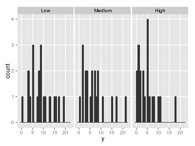
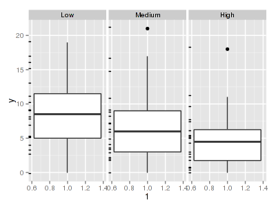
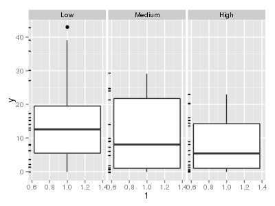
The potential for overdispersion can be explored by adding a rug to boxplot. The rug is simply tick marks on the inside of an axis at the position corresponding to an observation. As multiple identical values result in tick marks drawn over one another, it is typically a good idea to apply a slight amount of jitter (random displacement) to the values used by the rug.
> library(ggplot2)
> ggplot(data.hp, aes(x = y)) + geom_histogram() + facet_wrap(~treat)
> ggplot(data.hp, aes(y = y, x = 1)) + geom_boxplot() + geom_rug(position = "jitter", sides = "l") + facet_grid(~treat)
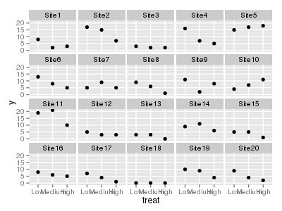
> ggplot(data.hp, aes(y = y, x = treat)) + geom_point() + facet_wrap(~sites)
Explore zero inflation
Although we have already established that there are few zeros in the data (and thus overdispersion is unlikely to be an issue), we can also explore this by comparing the number of zeros in the data to the number of zeros that would be expected from a Poisson distribution with a mean equal to the mean count of the data.
> # proportion of 0's in the data
> data.hp.tab <- table(data.hp$y == 0)
> data.hp.tab/sum(data.hp.tab)
  FALSE    TRUE
0.93333 0.06667
> # proportion of 0's expected from a Poisson distribution
> mu <- mean(data.hp$y)
> cnts <- rpois(1000, mu)
> data.hp.tab <- table(cnts == 0)
> data.hp.tab/sum(data.hp.tab)
FALSE  TRUE
0.999 0.001
6.7%) corresponds closely to the very low proportion expected (NA, NA%).
Model fitting or statistical analysis
As introduced at the start of this tutorial, Generalized Linear Mixed effects Models (GLMM) can be fit via numerous alternative processes. In a frequentist paradigm, the three most popular estimation routines are Penalized Quasi-likelihood (PQL), Laplace approximation and Gauss-Hermite quadrature (GHQ).
In R, the first of these (PQL) is provided by the glmmPQL() function in the MASS package whereas the later two are provided by the glmer() function in the lme4 package. As these functions are quite different to one another, I will tackle each separately.
PQL - glmmPQL
The most important (=commonly used) parameters/arguments for logistic regression are:- fixed: the linear model relating the response variable to the fixed components of the linear predictor
- random: the linear model relating the response variable to the random components of the linear predictor
- family: specification of the error distribution (and link function).
Can be specified as either a string or as one of the family functions (which allows for the explicit declaration of the link function).
For examples:
- family="poisson" or equivalently family=poisson(link="log")
- data: the data frame containing the data
> library(MASS)
> data.hp.glmmPQL <- glmmPQL(y ~ treat, random = ~1 | sites, data = data.hp, family = "poisson")
Laplace approximation - glmer
The most important (=commonly used) parameters/arguments for logistic regression are:- formula: the linear model relating the response variable to the linear predictor (fixed and random factors)
- family: specification of the error distribution (and link function).
Can be specified as either a string or as one of the family functions (which allows for the explicit declaration of the link function).
For examples:
- family="poisson" or equivalently family=poisson(link="log")
- data: the data frame containing the data
- nAGQ=1 indicates only a single quadrature point and therefore Laplace approximation (note, this is also the default and thus does not actually need to be specified).
> library(lme4)
> data.hp.glmerL <- glmer(y ~ treat + (1 | sites), data = data.hp, family = "poisson")  #Laplacian approximation
Gauss-Hermite quadrature - glmer
The most important (=commonly used) parameters/arguments for logistic regression are:- formula: the linear model relating the response variable to the linear predictor (fixed and random factors)
- family: specification of the error distribution (and link function).
Can be specified as either a string or as one of the family functions (which allows for the explicit declaration of the link function).
For examples:
- family="poisson" or equivalently family=poisson(link="log")
- data: the data frame containing the data
- nAGQ>1 specifies the number of quadrature points to use - the higher the number the more accurate the approximations will be.
> library(lme4)
> data.hp.glmerGHQ <- glmer(y ~ treat + (1 | sites), data = data.hp, family = "poisson", nAGQ = 7)  #Adaptive Gaussian Quadrature (L=7) gives same as Laplace here
Model evaluation
Expected values > 5
> predict(data.hp.glmmPQL, newdata = data.frame(treat = gl(3, 1, 3, c("Low", "Medium", "High"))), type = "response",
+     level = 0)
[1] 7.552 6.050 4.162
attr(,"label")
[1] "Predicted values"
> predict(data.hp.glmerL, newdata = data.frame(treat = gl(3, 1, 3, c("Low", "Medium", "High"))), REform = NA,
+     , type = "response")
    1     2     3
7.261 5.817 4.002
Residuals
Lets explore the diagnostics - particularly the residuals
> # glmmPQL
> plot(data.hp.glmmPQL)
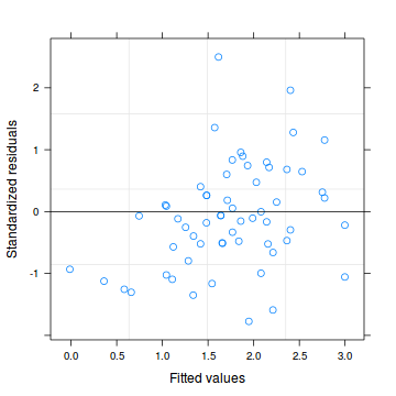
> ## OR
> plot(residuals(data.hp.glmmPQL, type = "pearson") ~ predict(data.hp.glmmPQL, type = "link"))

> plot(residuals(data.hp.glmmPQL, type = "pearson") ~ as.numeric(data.hp$treat))

> # Laplace plot(data.hp.glmerL)
> plot(residuals(data.hp.glmerL, type = "pearson") ~ predict(data.hp.glmerL, type = "link"))

> plot(residuals(data.hp.glmerL, type = "pearson") ~ as.numeric(data.hp$treat))

> # GHQ plot(data.hp.glmerGHQ)
> plot(residuals(data.hp.glmerGHQ, type = "pearson") ~ predict(data.hp.glmerGHQ, type = "link"))

> plot(residuals(data.hp.glmerGHQ, type = "pearson") ~ as.numeric(data.hp$treat))

Goodness of fit (and overdispersion) of the model
Estimating the dispersion parameter in GLMM is a reasonably tricky process. Essentially it involves calculating the ratio of the deviance (or sum of residual sums of squares) to the residual degrees of freedom. However, glmmPQL() (being an implementation of quasi-likelihood) strictly does not approximate the likelihood (and thus deviance) and the developers have gone to lengths to make the deviance difficult to obtain. On the other hand, glmer() developers have do not provide estimates of residual degrees of freedom.
Similarly, n order to estimate the goodness of fit and estimates of overdispersion we need to compare the sum of the squared residuals to chi squared. However, determining which chi squared distribution depends on having an estimation of the residual degrees of freedom. For PQL fits, residual degrees of freedom. is estimated via the 'Between-Within' method. For Laplace and GHQ fits (in R), no estimates of residual degrees of freedom are available.
Consequently, it is necessary to estimate this ourselves. A pragmatic approach is to calculate the degrees of freedom as the number of data rows minus the number of fixed effects minus one (for the residual term). This method considers the random effects as part of the residuals. Alternatively, the random effects could be considered as parameters in which case we could also subtract the number of levels of the random effects. We will adopt the former.
Ben Bolker has put together a FAQ [http://glmm.wikidot.com/faq] that provides numerous explanations and code snippets relating to issues of fitted GLMM's in R. On this page, he includes a small function that he has written that calculates the chi squared statistic, estimated residual degrees of freedom (assuming that the random effects are part of the residuals) and associated p-value for assessing overdispersion from models fit via glmer. This function also provides a measure of the dispersion statistic (ratio of sum of squared residuals to residual degrees of freedom). We can also explore the goodness of the fit of the model via:
- Pearson's $\chi^2$ residuals
- explores whether there are any significant patterns remaining in the residuals and in particular whether there is any evidence of overdispersion
Conclusions: the Pearson's residuals from neither model indicate a lack of fit or evidence of overdispersion (p values greater than 0.05).
> # PQL
> data.hp.resid <- sum(resid(data.hp.glmmPQL, type = "pearson")^2)
> 1 - pchisq(data.hp.resid, data.hp.glmmPQL$fixDF$X[2])
[1] 0.262
> # OR
> rdf <- length(data.hp.glmmPQL$data$y) - length(fixef(data.hp.glmmPQL)) - 1
> rdf
[1] 56
> 1 - pchisq(data.hp.resid, rdf)
[1] 0.8966
> data.hp.resid/rdf
[1] 0.7698
> # Laplace scale parameter (That quantity is the square root of the penalized residual sum of squares
> # divided by n, the number of observations)
> sqrt(sum(c(residuals(data.hp.glmerL), data.hp.glmerL@u)^2)/length(residuals(data.hp.glmerL)))
[1] 1.091
>
> data.hp.resid <- sum(resid(data.hp.glmerL, type = "pearson")^2)
> rdf <- nrow(model.frame(data.hp.glmerL)) - length(fixef(data.hp.glmerL)) - 1
> rdf
[1] 56
> 1 - pchisq(data.hp.resid, rdf)
[1] 0.772
> # OR using Ben Bolker's function
> overdisp_fun <- function(model) {
+     ## number of variance parameters in an n-by-n variance-covariance matrix
+     vpars <- function(m) {
+         nrow(m) * (nrow(m) + 1)/2
+     }
+     model.df <- sum(sapply(VarCorr(model), vpars)) + length(fixef(model))
+     rdf <- nrow(model.frame(model)) - model.df
+     rp <- residuals(model, type = "pearson")
+     Pearson.chisq <- sum(rp^2)
+     prat <- Pearson.chisq/rdf
+     pval <- pchisq(Pearson.chisq, df = rdf, lower.tail = FALSE)
+     c(chisq = Pearson.chisq, ratio = prat, rdf = rdf, p = pval)
+ }
>
> overdisp_fun(data.hp.glmerL)
  chisq   ratio     rdf       p
47.8657  0.8547 56.0000  0.7720
Exploring the model parameters, test hypotheses
If there was any evidence that the assumptions had been violated or the model was not an appropriate fit, then we would need to reconsider the model and start the process again. In this case, there is no evidence that the test will be unreliable so we can proceed to explore the test statistics. The main statistic of interest is the Wald statistic ($t$ for PQL $z$ for Laplace) for the fixed effects parameters.
Along with the parameter estimates (and there associated Wald tests), we can also investigate the influence of the factor as a whole. This is an approach analogous to ANOVA that explores the main effects. Since likelihood ratio tests (LRT) are inappropriate for PQL models, and LRT for fixed factors should only be based on models that employ REML (which is not currently available for GLMM in R), testing main effects is best done via Wald tests and the wald.test() function in the aod package.
The wald.test() function uses the fixed effects parameter estimates (b) along with the variance-covariance matrix (Sigma) and a specification of which fixed factor terms (Terms) to combine for the Wald statistic. In this case, to explore the overall effect of treatment, we need to combine factor effects 2 (the effect of the 'Medium' treatment) and 3 (the effect of the 'High treatment).
> summary(data.hp.glmmPQL)
Linear mixed-effects model fit by maximum likelihood
 Data: data.hp
  AIC BIC logLik
   NA  NA     NA

Random effects:
 Formula: ~1 | sites
        (Intercept) Residual
StdDev:      0.6235    1.067

Variance function:
 Structure: fixed weights
 Formula: ~invwt
Fixed effects: y ~ treat
              Value Std.Error DF t-value p-value
(Intercept)  2.0218    0.1677 38  12.054  0.0000
treatMedium -0.2217    0.1237 38  -1.793  0.0810
treatHigh   -0.5958    0.1384 38  -4.305  0.0001
 Correlation:
            (Intr) trtMdm
treatMedium -0.328
treatHigh   -0.293  0.398

Standardized Within-Group Residuals:
    Min      Q1     Med      Q3     Max
-1.7731 -0.5340 -0.1107  0.4205  2.4987

Number of Observations: 60
Number of Groups: 20
> library(aod) > wald.test(b=fixef(data.hp.glmmPQL), + Sigma=vcov(data.hp.glmmPQL),Terms=2:3)
Wald test:
----------

Chi-squared test:
X2 = 19.5, df = 2, P(> X2) = 5.8e-05
> intervals(data.hp.glmmPQL)
Approximate 95% confidence intervals

 Fixed effects:
              lower    est.    upper
(Intercept)  1.6909  2.0218  2.35279
treatMedium -0.4658 -0.2217  0.02232
treatHigh   -0.8688 -0.5958 -0.32272
attr(,"label")
[1] "Fixed effects:"

 Random Effects:
  Level: sites
                 lower   est.  upper
sd((Intercept)) 0.4123 0.6235 0.9429

 Within-group standard error:
lower  est. upper
0.847 1.067 1.343
> library(gmodels) > ci(data.hp.glmmPQL)
            Estimate CI lower CI upper Std. Error
(Intercept)   2.0218   1.6823  2.36139     0.1677
treatMedium  -0.2217  -0.4721  0.02866     0.1237
treatHigh    -0.5958  -0.8759 -0.31563     0.1384
            DF   p-value
(Intercept) 38 1.490e-14
treatMedium 38 8.099e-02
treatHigh   38 1.130e-04
> VarCorr(data.hp.glmmPQL)
sites = pdLogChol(1)
            Variance StdDev
(Intercept) 0.3888   0.6235
Residual    1.1377   1.0666
> summary(data.hp.glmerL)
Generalized linear mixed model fit by maximum likelihood ['glmerMod']
 Family: poisson ( log )
Formula: y ~ treat + (1 | sites)
   Data: data.hp

     AIC      BIC   logLik deviance
   326.0    334.4   -159.0    318.0

Random effects:
 Groups Name        Variance Std.Dev.
 sites  (Intercept) 0.435    0.66
Number of obs: 60, groups: sites, 20

Fixed effects:
            Estimate Std. Error z value Pr(>|z|)
(Intercept)    1.983      0.168   11.79  < 2e-16
treatMedium   -0.222      0.113   -1.96     0.05
treatHigh     -0.596      0.127   -4.71  2.5e-06

(Intercept) ***
treatMedium .
treatHigh   ***
---
Signif. codes:
0 '***' 0.001 '**' 0.01 '*' 0.05 '.' 0.1 ' ' 1

Correlation of Fixed Effects:
            (Intr) trtMdm
treatMedium -0.299
treatHigh   -0.267  0.398
> library(aod) > wald.test(b=fixef(data.hp.glmerL), + Sigma=vcov(data.hp.glmerL),Terms=2:3)
Wald test:
----------

Chi-squared test:
X2 = 22.1, df = 2, P(> X2) = 1.6e-05
> anova(data.hp.glmerL)
Analysis of Variance Table
      Df Sum Sq Mean Sq F value
treat  2   22.1    11.1    11.1
> confint(data.hp.glmerL)
              2.5 %     97.5 %
.sig01       0.4485  1.0175132
(Intercept)  1.6171  2.3176814
treatMedium -0.4444 -0.0008816
treatHigh   -0.8469 -0.3505665
> VarCorr(data.hp.glmerL)
 Groups Name        Std.Dev.
 sites  (Intercept) 0.66
Conclusions: Via either method we would reject the null hypothesis (p<0.05 from the global Wald test). The individual effects parameters suggest that the response is significantly higher for the 'Low' treatment effect than the 'High' treatment effect, yet was not found to be different between the 'Low' and 'Medium' treatments.
Note, the effect sizes (provided in the Fixed effects coefficients tables) are on a log scale since by default the Poisson distribution uses a log-link function.
Coefficient of determination ($R^2$) analogue
Unlike simple linear regression in which the $R^2$ value (ratio of explained variability to total variability) neatly encapsulates a property that we can interpret as the proportion of variability explained by a model, simple analogues for GLM and LMM (and thus GLMM) are not available. In part this is because it is difficult to know how to include all the sources of random variation (random effects and residuals).
Nevertheless, we can generate quasi-$R^2$ values by calculating the ratio of variance in the residuals to total variance in the response:
> #PQL
> #totalss <- var(resid(data.hp.glmmPQL)+fitted(data.hp.glmmPQL))
> totalss <- var(resid(data.hp.glmmPQL,type='pearson')+predict(data.hp.glmmPQL, type='link'))
> 1-var(residuals(data.hp.glmmPQL, type='pearson'))/(totalss)
[1] 0.5101
> #Laplace
> #totalss <- var(resid(data.hp.glmerL)+fitted(data.hp.glmerL))
> totalss <- var(resid(data.hp.glmerL, type='pearson')+predict(data.hp.glmerL, type='link'))
> 1-var(residuals(data.hp.glmerL, type='pearson'))/(totalss)
[1] 0.4974
Summary plot
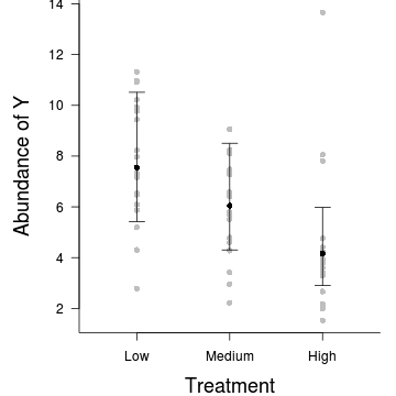
Note, plotting the raw data, is of little value when there are large effects of the random effects (sites) since the spread of points will say more about the variability between sites than the variability due the treatments. If you wish to plot something in addition to the modelled summaries (means and confidence intervals), one sensible option would be to plot the result of adding the residuals to the fitted values.
> par(mar = c(4, 5, 0, 1))
> res <- exp(predict(data.hp.glmmPQL, level = 0) + residuals(data.hp.glmmPQL))
> plot.default(res ~ treat, data = data, xlim = c(0.5, 3.5), type = "n", ann = F, axes = F)
> points(res ~ treat, data = data.hp, pch = 16, col = "grey")
> coefs <- fixef(data.hp.glmmPQL)
> pred <- data.frame(treat = gl(3, 1, 3, c("Low", "Medium", "High")))
> mm <- model.matrix(~treat, data = pred)
> fit <- as.vector(coefs %*% t(mm))
> pred$fit <- exp(fit)
> se <- sqrt(diag(mm %*% vcov(data.hp.glmmPQL) %*% t(mm)))
> pred$lwr <- exp(fit - qt(0.975, data.hp.glmmPQL$fixDF$X[2]) * se)
> pred$upr <- exp(fit + qt(0.975, data.hp.glmmPQL$fixDF$X[2]) * se)
> points(fit ~ treat, data = pred, pch = 16)
> with(pred, arrows(as.numeric(treat), lwr, as.numeric(treat), upr, code = 3, angle = 90,
+     length = 0.1))
> axis(1, at = 1:3, lab = c("Low", "Medium", "High"))
> mtext("Treatment", 1, cex = 1.5, line = 3)
> axis(2, las = 2)
> mtext("Abundance of Y", 2, cex = 1.5, line = 3)
> box(bty = "l")
Hierarchical Quasi-Poisson regression
Scenario and Data
Consider an experimental design in which we wished to measure of the abundance of individuals of a species (or number of incidents etc) in response to some categorical influence (such as level of exposure to some disturbance(s) - 'high','medium', 'low'). In an attempt to minimize the expected extent of unexplained variability (due to highly heterogeneous underlying conditions across the landscape), each of the exposure 'treatments' were applied within a relatively small spatial scale (individual sites) - that is, they were blocked. In all, we will employ 20 randomly (or haphazardly selected) sites and the treatments will be applied randomly (or haphazardly) within sites.
Random data incorporating the following trends (effect parameters)- the number of sites ($sites$) = 20
- the categorical treatment $treat$ variable comprising of three levels ('High', 'Medium' and 'Low')
- the mean value of $y$ of the 'low' treatment is 8
- the standard deviation in 'low' treatment $y$ values across the 20 sites is 0.5
- the mean effect of the 'Medium' effect is -1
- the mean effect of the 'High' effect is -2
- to generate the values of $y$ expected at each $treat$ level within each of the $sites$, we evaluate the linear predictor (created by calculating the outer product of the model matrix and the regression parameters). These expected values are then transformed into a scale mapped by (0,$\infty$) by using the log function $e^{linear~predictor}$
- finally, we generate $y$ values by using the expected $y$ values ($\lambda$) as probabilities when drawing random numbers from a Poisson distribution. This step adds random noise to the expected $y$ values and returns only 0's and positive integers.
> # Quasi-poisson distrition
> rqpois <- function(n, lambda, phi) {
+     mu = lambda
+     r = rnbinom(n, size = mu/phi/(1 - 1/phi), prob = 1/phi)
+     return(r)
+ }
> set.seed(321)  #4
> # number of sites
> n.sites <- 20
> n.treat <- 3
> n <- n.sites * n.treat
> sites <- gl(n = n.sites, k = n.treat, lab = paste("Site", 1:n.sites, sep = ""))
> treat <- gl(n = n.treat, 1, n, lab = c("Low", "Medium", "High"))
> # Xmat <- model.matrix(~sites*treat-1-treat)
> Xmat <- model.matrix(~-1 + sites + treat)
>
> intercept.mean <- 12  # mu alpha
> intercept.sd <- 5  # sigma alpha
> # effect.sd <- 1.1
> treatM.effect <- -3
> treatH.effect <- -5
> intercept.effects <- rnorm(n = n.sites, mean = intercept.mean, sd = intercept.sd)
> # treatM.effects <- rnorm(n=n.sites, mean=treatM.effect, sd=effect.sd)
> # treatH.effects <- rnorm(n=n.sites, mean=treatH.effect, sd=effect.sd)
> all.effects <- c(intercept.effects, treatM.effect, treatH.effect)  # Put them all together
> lin.pred <- Xmat[, ] %*% all.effects
> lin.pred[lin.pred < 0] <- exp(lin.pred[lin.pred < 0])
> y <- rqpois(n = n, lambda = lin.pred, phi = 6)  #as.integer(lin.pred+eps)
> data.hqp <- data.frame(y, treat, sites)
> head(data.hqp)
   y  treat sites
1 27    Low Site1
2 19 Medium Site1
3  1   High Site1
4  0    Low Site2
5  0 Medium Site2
6  0   High Site2
> write.table(data.hqp, file = "../downloads/data/data.hqp.csv", quote = F, row.names = F,
+     sep = ",")
Exploratory data analysis and initial assumption checking
The assumptions are:- All of the observations are independent - the blocking design will introduce a dependency structure (observations within each block are not strictly independent) that we need to address via mixed effects modelling.
- The response variable (and thus the residuals) should be matched by an appropriate distribution (in the case of positive integers response - a Poisson is appropriate).
- All observations are equally influential in determining the trends - or at least no observations are overly influential. This is most effectively diagnosed via residuals and other influence indices and is very difficult to diagnose prior to analysis
- the relationship between the linear predictor (right hand side of the regression formula) and the link function should be linear. A scatterplot with smoother can be useful for identifying possible non-linearity.
- If using a Poisson distribution, the dispersion factor is close to 1
There are (at least) five main potential models we could consider fitting to these data:
- Ordinary least squares ANOVA (generalized least squares model) - assumes normality and homogeneity of variance of residuals as well as an absence of a dependency structure
- Linear mixed effects model - assumes normality and homogeneity of variance of residuals
- Poisson mixed effects model - assumes mean=variance (dispersion=1)
- Quasi-poisson mixed effects model - a general solution to overdispersion. Assumes variance is a function of mean, dispersion estimated, however likelihood based statistics unavailable
- Negative binomial mixed effects model - a specific solution to overdispersion caused by clumping (due to an unmeasured latent variable). Scaling factor ($\omega$) is estimated along with the regression parameters.
- Zero-inflation mixed effects model - a specific solution to overdispersion caused by excessive zeros (due to an unmeasured latent variable). Mixture of binomial and Poisson mixed effects models.
Confirm non-normality and explore clumping
When counts are all very large (not close to 0) and their ranges do not span orders of magnitude, they take on very Gaussian-like properties (symmetrical distribution and variance independent of the mean). Given that models based on the Gaussian distribution are more optimized and recognized than Generalized Linear Mixed Effects Models (GLMM), it can be prudent to adopt Gaussian models for such data. Hence it is a good idea to first explore whether a Poisson model is likely to be more appropriate than a standard Gaussian model.
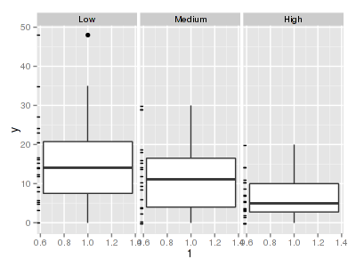
The potential for overdispersion can be explored by adding a rug to boxplot. The rug is simply tick marks on the inside of an axis at the position corresponding to an observation. As multiple identical values result in tick marks drawn over one another, it is typically a good idea to apply a slight amount of jitter (random displacement) to the values used by the rug.
There are signs of non-normality that would warrant Poisson models. The rug applied to the boxplots does not indicate a serious degree of clumping and there appears to be few zeros. So if there is overdispersion it is unlikely that it is due to either clumping or excessive zeros.> library(ggplot2) > ggplot(data.hqp, aes(x = y)) + geom_histogram() + facet_wrap(~treat)
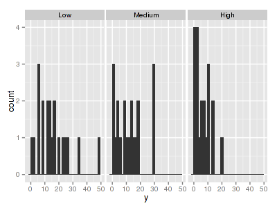
> ggplot(data.hqp, aes(y = y, x = 1)) + geom_boxplot() + geom_rug(position = "jitter",
+     sides = "l") + facet_grid(~treat)
> ggplot(data.hqp, aes(y = y, x = treat)) + geom_point() + facet_wrap(~sites)

Explore zero inflation
Although we have already established that there are few zeros in the data (and thus overdispersion is unlikely to be an issue), we can also explore this by comparing the number of zeros in the data to the number of zeros that would be expected from a Poisson distribution with a mean equal to the mean count of the data.
In the above, the value under FALSE is the proportion of non-zero values in the data and the value under TRUE is the proportion of zeros in the data. In this example, the observed proportion (> # proportion of 0's in the data1 > data.hqp.tab <- table(data.hqp$y == 0) > data.hqp.tab/sum(data.hqp.tab)
 FALSE   TRUE
0.8833 0.1167
> # proportion of 0's expected from a Poisson distribution
> mu <- mean(data.hqp$y)
> cnts <- rpois(1000, mu)
> data.hqp.tab <- table(cnts == 0)
> data.hqp.tab/sum(data.hqp.tab)
FALSE 111.7%) is not substantially higher than the expected number of zeros (0.0%).Model fitting or statistical analysis
As introduced at the start of this tutorial, Generalized Linear Mixed effects Models (GLMM) can be fit via numerous alternative processes. In a frequentist paradigm, the three most popular estimation routines are Penalized Quasi-likelihood (PQL), Laplace approximation and Gauss-Hermite quadrature (GHQ).
At this point, we could fit a Poisson mixed effects model and explore the fit of the model (particularly with respect to overdispersion and residuals). For the purpose of this tutorial, we will assume that the data are overdispersed. However, if you expand the following section, you will be able to see the data fit with a Poisson model and the diagnostics.
> # PQL
> library(MASS)
> data.hqp.glmmPQL <- glmmPQL(y ~ treat, random = list(~1 | sites), data = data.hqp,
+     family = "poisson")
> # Laplace
> library(lme4)
> data.hqp.glmerL <- glmer(y ~ treat + (1 | sites), data = data.hqp, family = "poisson")  #Laplacian approximation
> # Laplace (via glmmADMB)
> library(glmmADMB)
> data.hqp.admb <- glmmadmb(y ~ treat + (1 | sites), family = "poisson", data = data.hqp)
> # Note that glmer and glmmadmb for simple Laplace balanced GLMM are identical,
> # therefore I will cease to present the glmmADMB model
Model evaluation
Expected values > 5
Conclusions: the expected values are all greater than 5 and thus PQL is likely to yield reasonably good approximations.> # from PQL > predict(data.hqp.glmmPQL, newdata = data.frame(treat = gl(3, 1, 3, c("Low", "Medium", + "High"))), type = "response", level = 0)
[1] 14.042 10.722  5.742
attr(,"label")
[1] "Predicted values"
> # from Laplace
> predict(data.hqp.glmerL, newdata = data.frame(treat = gl(3, 1, 3, c("Low", "Medium",
+     "High"))), REform = NA, type = "response")
     1      2      3
12.195  9.312  4.987
Lets explore the diagnostics - particularly the residuals
Conclusions: there are no immediately obvious patterns in the residuals. All three approximation techniques yield very similar residuals.> plot(data.hqp.glmmPQL)
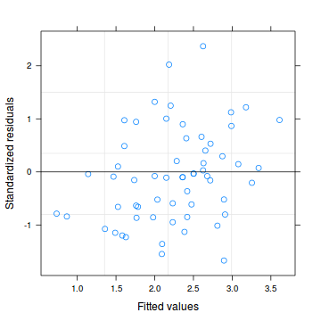
> # OR
> plot(residuals(data.hqp.glmmPQL, type = "pearson") ~ predict(data.hqp.glmmPQL, type = "link"))

> plot(residuals(data.hqp.glmmPQL, type = "pearson") ~ as.numeric(data.hqp$treat))

> # Laplace plot(data.hqp.glmerL)
> plot(residuals(data.hp.glmerL, type = "pearson") ~ predict(data.hp.glmerL, type = "link"))

> plot(residuals(data.hqp.glmerL, type = "pearson") ~ as.numeric(data.hqp$treat))

Goodness of fit (and overdispersion) of the model
Conclusions: there is some evidence that the data are overdispersed and that a regular Poisson distribution does not adequately capture all of the variance in the data.> # PQL > data.hqp.resid <- sum(resid(data.hqp.glmmPQL, type = "pearson")^2) > rdf <- length(data.hqp.glmmPQL$data$y) - length(fixef(data.hqp.glmmPQL)) - 1 > 1 - pchisq(data.hqp.resid, rdf)
[1] 0.8419
> data.hqp.resid/rdf
[1] 0.8118
> # Laplace
> data.hqp.resid <- sum(resid(data.hqp.glmerL, type = "pearson")^2)
> rdf <- nrow(model.frame(data.hqp.glmerL)) - length(fixef(data.hqp.glmerL)) - 1
> 1 - pchisq(data.hqp.resid, rdf)
[1] 4.427e-08
> # OR using Ben Bolker's function
> overdisp_fun <- function(model) {
+     ## number of variance parameters in an n-by-n variance-covariance matrix
+     vpars <- function(m) {
+         nrow(m) * (nrow(m) + 1)/2
+     }
+     model.df <- sum(sapply(VarCorr(model), vpars)) + length(fixef(model))
+     rdf <- nrow(model.frame(model)) - model.df
+     rp <- residuals(model, type = "pearson")
+     Pearson.chisq <- sum(rp^2)
+     prat <- Pearson.chisq/rdf
+     pval <- pchisq(Pearson.chisq, df = rdf, lower.tail = FALSE)
+     c(chisq = Pearson.chisq, ratio = prat, rdf = rdf, p = pval)
+ }
>
> overdisp_fun(data.hqp.glmerL)
    chisq     ratio       rdf         p
1.320e+02 2.357e+00 5.600e+01 4.427e-08
The focus of this demonstration will be on fitting a Quasi-Poisson mixed effects model. Simulations by Ben Bolker have indicated that glmer does not consistently perform correctly with Quasi family distributions. Instead, lme4 developers are now advocating the use of observation-level random effects (the focus of the next major section in the tutorial).
In R, the first of these (PQL) is provided by the glmmPQL() function in the MASS package whereas the later two are provided by the glmer() function in the lme4 package. As these functions are quite different to one another, I will tackle each separately.
> library(MASS)
> data.hqp.glmmPQL <- glmmPQL(y ~ treat, random = list(~1 | sites), data = data.hqp,
+     family = quasipoisson(link = log))
Model evaluation
Expected values > 5
Conclusions: the expected values are all greater than 5 and thus PQL is likely to yield reasonably good approximations.> predict(data.hqp.glmmPQL, newdata = data.frame(treat = gl(3, 1, 3, c("Low", "Medium", + "High"))), type = "response", level = 0)
[1] 14.042 10.722  5.742
attr(,"label")
[1] "Predicted values"
Lets explore the diagnostics - particularly the residuals
Conclusions: there are no immediately obvious patterns in the residuals. All three approximation techniques yield very similar residuals.> plot(data.hqp.glmmPQL)

> plot(residuals(data.hqp.glmmPQL, type = "pearson") ~ as.numeric(data.hqp$treat))

Goodness of fit (and overdispersion) of the model
- Pearson's $\chi^2$ residuals
- explores whether there are any significant patterns remaining in the residuals and in particular whether there is any evidence of overdispersion
> # PQL
> data.hqp.resid <- sum(resid(data.hqp.glmmPQL, type = "pearson")^2)
> # str(data.glmmPQL)
> rdf <- length(data.hqp.glmmPQL$data$y) - length(fixef(data.hqp.glmmPQL)) - 1
> rdf
[1] 56
> 1 - pchisq(data.hqp.resid, rdf)
[1] 0.8419
>
> data.hqp.resid/(nrow(data.hqp) - length(fixef(data.hqp.glmmPQL)) - 1)
[1] 0.8118
Exploring the model parameters, test hypotheses
If there was any evidence that the assumptions had been violated or the model was not an appropriate fit, then we would need to reconsider the model and start the process again. In this case, there is no evidence that the test will be unreliable so we can proceed to explore the test statistics. The main statistic of interest is the Wald statistic ($t$ for PQL) for the fixed effects parameters.
Along with the parameter estimates (and there associated Wald tests), we can also investigate the influence of the factor as a whole. This is an approach analogous to ANOVA that explores the main effects. Since likelihood ratio tests (LRT) are inappropriate for PQL models, and LRT for fixed factors should only be based on models that employ REML (which is not currently available for GLMM in R), testing main effects is best done via Wald tests and the wald.test() function in the aod package.
The wald.test() function uses the fixed effects parameter estimates (b) along with the variance-covariance matrix (Sigma) and a specification of which fixed factor terms (Terms) to combine for the Wald statistic. In this case, to explore the overall effect of treatment, we need to combine factor effects 2 (the effect of the 'Medium' treatment) and 3 (the effect of the 'High treatment).
> summary(data.hqp.glmmPQL)
Linear mixed-effects model fit by maximum likelihood
 Data: data.hqp
  AIC BIC logLik
   NA  NA     NA

Random effects:
 Formula: ~1 | sites
        (Intercept) Residual
StdDev:      0.5574    1.841

Variance function:
 Structure: fixed weights
 Formula: ~invwt
Fixed effects: y ~ treat
              Value Std.Error DF t-value p-value
(Intercept)  2.6420    0.1693 38  15.610  0.0000
treatMedium -0.2697    0.1622 38  -1.663  0.1046
treatHigh   -0.8942    0.1981 38  -4.513  0.0001
 Correlation:
            (Intr) trtMdm
treatMedium -0.415
treatHigh   -0.340  0.354

Standardized Within-Group Residuals:
     Min       Q1      Med       Q3      Max
-1.66946 -0.79020 -0.09365  0.49892  2.36924

Number of Observations: 60
Number of Groups: 20
> library(aod) > wald.test(b = fixef(data.hqp.glmmPQL), Sigma = vcov(data.hqp.glmmPQL), Terms = 2:3)
Wald test:
----------

Chi-squared test:
X2 = 21.4, df = 2, P(> X2) = 2.2e-05
> intervals(data.hqp.glmmPQL)
Approximate 95% confidence intervals

 Fixed effects:
              lower    est.    upper
(Intercept)  2.3081  2.6420  2.97601
treatMedium -0.5898 -0.2697  0.05037
treatHigh   -1.2851 -0.8942 -0.50321
attr(,"label")
[1] "Fixed effects:"

 Random Effects:
  Level: sites
                lower   est.  upper
sd((Intercept)) 0.342 0.5574 0.9086

 Within-group standard error:
lower  est. upper
1.462 1.841 2.318
> library(gmodels) > ci(data.hqp.glmmPQL)
            Estimate CI lower CI upper Std. Error DF   p-value
(Intercept)   2.6420   2.2994  2.98468     0.1693 38 4.073e-18
treatMedium  -0.2697  -0.5982  0.05868     0.1622 38 1.046e-01
treatHigh    -0.8942  -1.2953 -0.49305     0.1981 38 6.004e-05
> VarCorr(data.hqp.glmmPQL)
sites = pdLogChol(1)
            Variance StdDev
(Intercept) 0.3107   0.5574
Residual    3.3892   1.8410
Conclusions: Via either method we would reject the null hypothesis (p<0.05 from the global Wald test). The individual effects parameters suggest that the response is significantly higher for the 'Low' treatment effect than the 'High' treatment effect, yet was not found to be different between the 'Low' and 'Medium' treatments.
Note, the effect sizes (provided in the Fixed effects coefficients tables) are on a log scale since by default the Poisson distribution uses a log-link function.
Coefficient of determination ($R^2$) analogue
Unlike simple linear regression in which the $R^2$ value (ratio of explained variability to total variability) neatly encapsulates a property that we can interpret as the proportion of variability explained by a model, simple analogues for GLM and LMM (and thus GLMM) are not available. In part this is because it is difficult to know how to include all the sources of random variation (random effects and residuals).
Nevertheless, we can generate quasi-$R^2$ values by calculating the ratio of variance in the residuals to total variance in the response:
> totalss <- var(resid(data.hqp.glmmPQL, type='pearson')+predict(data.hqp.glmmPQL, type='link'))
> 1-var(residuals(data.hqp.glmmPQL, type='pearson'))/(totalss)
[1] 0.4698
Summary plot
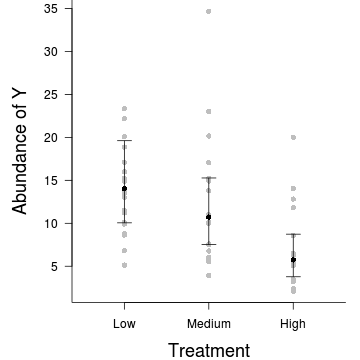
> par(mar = c(4, 5, 0, 1))
> res <- exp(predict(data.hqp.glmmPQL, level = 0) + residuals(data.hqp.glmmPQL))
> plot.default(res ~ treat, data = data.hqp, xlim = c(0.5, 3.5), type = "n", ann = F,
+     axes = F)
> points(res ~ treat, data = data.hqp, pch = 16, col = "grey")
> coefs <- fixef(data.hqp.glmmPQL)
> pred <- data.frame(treat = gl(3, 1, 3, c("Low", "Medium", "High")))
> mm <- model.matrix(~treat, data = pred)
> fit <- as.vector(coefs %*% t(mm))
> pred$fit <- exp(fit)
> se <- sqrt(diag(mm %*% vcov(data.hqp.glmmPQL) %*% t(mm)))
> pred$lwr <- exp(fit - qt(0.975, data.hqp.glmmPQL$fixDF$X[2]) * se)
> pred$upr <- exp(fit + qt(0.975, data.hqp.glmmPQL$fixDF$X[2]) * se)
> points(fit ~ treat, data = pred, pch = 16)
> with(pred, arrows(as.numeric(treat), lwr, as.numeric(treat), upr, code = 3, angle = 90,
+     length = 0.1))
> axis(1, at = 1:3, lab = c("Low", "Medium", "High"))
> mtext("Treatment", 1, cex = 1.5, line = 3)
> axis(2, las = 2)
> mtext("Abundance of Y", 2, cex = 1.5, line = 3)
> box(bty = "l")
Hierarchical Poisson regression with observation-level random effects
We will use the same data from above and thus the data exploration is identical to that illustrated above.
Model fitting or statistical analysis
> data.hob <- data.hqp
> data.hob$Obs <- factor(1:nrow(data.hob))
> # PQL
> library(MASS)
> data.hob.glmmPQL <- glmmPQL(y ~ treat, random = list(~1 | sites, ~1 | Obs), data = data.hob,
+     family = quasipoisson(link = log))
> # Laplace
> library(lme4)
> data.hob.glmerL <- glmer(y ~ treat + (1 | sites) + (1 | Obs), data = data.hob, family = "poisson")
> # ADMB
> library(glmmADMB)
> data.hob.admb <- glmmadmb(y ~ treat + (1 | sites) + (1 | Obs), data = data.hob, family = "poisson")
Expected values > 5
Conclusions: the expected values are all greater than 5 and thus PQL is likely to yield reasonably good approximations.> # from PQL > predict(data.hob.glmmPQL, newdata = data.frame(treat = gl(3, 1, 3, c("Low", "Medium", + "High"))), type = "response", level = 0)
[1] 13.590 10.367  5.685
attr(,"label")
[1] "Predicted values"
> # from Laplace
> predict(data.hob.glmerL, newdata = data.frame(treat = gl(3, 1, 3, c("Low", "Medium",
+     "High"))), REform = NA, type = "response")
     1      2      3
11.571  8.283  4.495
> # from Laplace
> predict(data.hob.admb, newdata = data.frame(treat = gl(3, 1, 3, c("Low", "Medium",
+     "High"))), REform = NA, type = "response")
[1] 11.569 8.281 4.491
Lets explore the diagnostics - particularly the residuals
Conclusions: there are no immediately obvious patterns in the residuals. All three approximation techniques yield very similar residuals.> plot(data.hob.glmmPQL)
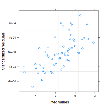
> plot(residuals(data.hob.glmmPQL, type = "pearson") ~ predict(data.hob.glmmPQL, type = "link"))

> plot(residuals(data.hob.glmmPQL, type = "pearson") ~ as.numeric(data.hob$treat))

>
> # Laplace
> plot(data.hob.glmerL)

> plot(residuals(data.hob.glmerL, type = "pearson") ~ predict(data.hob.glmerL, type = "link"))

> plot(residuals(data.hob.glmerL, type = "pearson") ~ as.numeric(data.hob$treat))

>
> # ADM
> plot(resid(data.hob.admb, type = "pearson") ~ predict(data.hob.admb, type = "link"))

> plot(residuals(data.hob.admb, type = "pearson") ~ as.numeric(data.hob$treat))

Exploring the model parameters, test hypotheses
> summary(data.hob.glmmPQL)
Linear mixed-effects model fit by maximum likelihood
 Data: data.hob
  AIC BIC logLik
   NA  NA     NA

Random effects:
 Formula: ~1 | sites
        (Intercept)
StdDev:      0.5527

 Formula: ~1 | Obs %in% sites
        (Intercept)  Residual
StdDev:      0.4772 0.0001938

Variance function:
 Structure: fixed weights
 Formula: ~invwt
Fixed effects: y ~ treat
              Value Std.Error DF t-value p-value
(Intercept)  2.6093    0.1675 38  15.576  0.0000
treatMedium -0.2707    0.1548 38  -1.748  0.0885
treatHigh   -0.8715    0.1548 38  -5.629  0.0000
 Correlation:
            (Intr) trtMdm
treatMedium -0.462
treatHigh   -0.462  0.500

Standardized Within-Group Residuals:
       Min         Q1        Med         Q3
-2.373e-04 -8.653e-05 -8.213e-06  6.891e-05
       Max
 2.517e-04

Number of Observations: 60
Number of Groups:
         sites Obs %in% sites
            20             60
> library(aod) > wald.test(b=fixef(data.hob.glmmPQL), + Sigma=vcov(data.hob.glmmPQL),Terms=2:3)
Wald test:
----------

Chi-squared test:
X2 = 34.9, df = 2, P(> X2) = 2.6e-08
> intervals(data.hob.glmmPQL)
Error: cannot get confidence intervals on var-cov
components: Non-positive definite approximate
variance-covariance
> library(gmodels)
> ci(data.hob.glmmPQL)
            Estimate CI lower CI upper Std. Error
(Intercept)   2.6093   2.2702  2.94846     0.1675
treatMedium  -0.2707  -0.5842  0.04273     0.1548
treatHigh    -0.8715  -1.1849 -0.55805     0.1548
            DF   p-value
(Intercept) 38 4.374e-18
treatMedium 38 8.846e-02
treatHigh   38 1.840e-06
> VarCorr(data.hob.glmmPQL)
            Variance     StdDev
sites =     pdLogChol(1)
(Intercept) 3.055e-01    0.5526874
Obs =       pdLogChol(1)
(Intercept) 2.277e-01    0.4772214
Residual    3.756e-08    0.0001938
> summary(data.hob.glmerL)
Generalized linear mixed model fit by maximum likelihood ['glmerMod']
 Family: poisson ( log )
Formula: y ~ treat + (1 | sites) + (1 | Obs)
   Data: data.hob

     AIC      BIC   logLik deviance
   410.9    421.4   -200.5    400.9

Random effects:
 Groups Name        Variance Std.Dev.
 Obs    (Intercept) 0.285    0.534
 sites  (Intercept) 0.599    0.774
Number of obs: 60, groups: Obs, 60; sites, 20

Fixed effects:
            Estimate Std. Error z value Pr(>|z|)
(Intercept)    2.448      0.222   11.02  < 2e-16
treatMedium   -0.334      0.200   -1.67    0.094
treatHigh     -0.946      0.210   -4.50  6.7e-06

(Intercept) ***
treatMedium .
treatHigh   ***
---
Signif. codes:
0 '***' 0.001 '**' 0.01 '*' 0.05 '.' 0.1 ' ' 1

Correlation of Fixed Effects:
            (Intr) trtMdm
treatMedium -0.427
treatHigh   -0.404  0.453
> library(aod) > wald.test(b=fixef(data.hob.glmerL), + Sigma=vcov(data.hob.glmerL),Terms=2:3)
Wald test:
----------

Chi-squared test:
X2 = 20.4, df = 2, P(> X2) = 3.7e-05
> anova(data.hob.glmerL)
Analysis of Variance Table
      Df Sum Sq Mean Sq F value
treat  2   20.4    10.2    10.2
> confint(data.hob.glmerL)
              2.5 %   97.5 %
.sig01       0.3694  0.76088
.sig02       0.4720  1.24557
(Intercept)  1.9750  2.89330
treatMedium -0.7533  0.06495
treatHigh   -1.3846 -0.52754
> VarCorr(data.hob.glmerL)
 Groups Name        Std.Dev.
 Obs    (Intercept) 0.534
 sites  (Intercept) 0.774
Coefficient of determination ($R^2$) analogue
> #PQL
> totalss <- var(resid(data.hob.glmmPQL, type='pearson')+predict(data.hob.glmmPQL, type='link'))
> 1-var(residuals(data.hob.glmmPQL, type='pearson'))/(totalss)
[1] 1
> #Laplace
> totalss <- var(resid(data.hob.glmerL)+fitted(data.hob.glmerL))
> 1-var(residuals(data.hob.glmerL))/(totalss)
[1] 0.9948
Summary plot
Note, plotting the raw data, is of little value when there are large effects of the random effects (sites) since the spread of points will say more about the variability between sites than the variability due the treatments. If you wish to plot something in addition to the modelled summaries (means and confidence intervals), one sensible option would be to plot the result of adding the residuals to the fitted values.
> par(mar = c(4, 5, 0, 1))
> res <- exp(predict(data.hob.glmmPQL, level = 0) + residuals(data.hob.glmmPQL))
> plot.default(res ~ treat, data = data.hob, xlim = c(0.5, 3.5), type = "n", ann = F,
+     axes = F)
> points(res ~ treat, data = data.hob, pch = 16, col = "grey")
> coefs <- fixef(data.hob.glmmPQL)
> pred <- data.frame(treat = gl(3, 1, 3, c("Low", "Medium", "High")))
> mm <- model.matrix(~treat, data = pred)
> fit <- as.vector(coefs %*% t(mm))
> pred$fit <- exp(fit)
> se <- sqrt(diag(mm %*% vcov(data.hob.glmmPQL) %*% t(mm)))
> pred$lwr <- exp(fit - qt(0.975, data.hob.glmmPQL$fixDF$X[2]) * se)
> pred$upr <- exp(fit + qt(0.975, data.hob.glmmPQL$fixDF$X[2]) * se)
> points(fit ~ treat, data = pred, pch = 16)
> with(pred, arrows(as.numeric(treat), lwr, as.numeric(treat), upr, code = 3, angle = 90,
+     length = 0.1))
> axis(1, at = 1:3, lab = c("Low", "Medium", "High"))
> mtext("Treatment", 1, cex = 1.5, line = 3)
> axis(2, las = 2)
> mtext("Abundance of Y", 2, cex = 1.5, line = 3)
> box(bty = "l")

Hierarchical negative binomial
Consider again the experimental design in which we wished to measure of the abundance of individuals of a species (or number of incidents etc) in response to some categorical influence (such as level of exposure to some disturbance(s) - 'high','medium', 'low'). In an attempt to minimize the expected extent of unexplained variability (due to highly heterogeneous underlying conditions across the landscape), each of the exposure 'treatments' were applied within a relatively small spatial scale (individual sites) - that is, they were blocked. In all, we will employ 20 randomly (or haphazardly selected) sites and the treatments will be applied randomly (or haphazardly) within sites.
Random data incorporating the following trends (effect parameters)- the number of sites ($sites$) = 20
- the categorical treatment $treat$ variable comprising of three levels ('High', 'Medium' and 'Low')
- the mean value of $y$ of the 'low' treatment is 8
- the standard deviation in 'low' treatment $y$ values across the 20 sites is 0.5
- the mean effect of the 'Medium' effect is -1
- the mean effect of the 'High' effect is -2
- to generate the values of $y$ expected at each $treat$ level within each of the $sites$, we evaluate the linear predictor (created by calculating the outer product of the model matrix and the regression parameters). These expected values are then transformed into a scale mapped by (0,$\infty$) by using the log function $e^{linear~predictor}$
- finally, we generate $y$ values by using the expected $y$ values ($\lambda$) as probabilities when drawing random numbers from a Poisson distribution. This step adds random noise to the expected $y$ values and returns only 0's and positive integers.
> set.seed(1)  #3 #7
> # number of sites
> n.sites <- 20
> n.treat <- 3
> n <- n.sites * n.treat
> sites <- gl(n = n.sites, k = n.treat, lab = paste("Site", 1:n.sites, sep = ""))
> treat <- gl(n = n.treat, 1, n, lab = c("Low", "Medium", "High"))
> # Xmat <- model.matrix(~sites*treat-1-treat)
> Xmat <- model.matrix(~-1 + sites + treat)
>
> intercept.mean <- 15  # mu alpha
> intercept.sd <- 5  # sigma alpha
> # effect.sd <- 1
> treatM.effect <- -4
> treatH.effect <- -8
> intercept.effects <- rnorm(n = n.sites, mean = intercept.mean, sd = intercept.sd)
> # treatM.effects <- rnorm(n=n.sites, mean=treatM.effect, sd=effect.sd)
> # treatH.effects <- rnorm(n=n.sites, mean=treatH.effect, sd=effect.sd)
> all.effects <- c(intercept.effects, treatM.effect, treatH.effect)  # Put them all together
> lin.pred <- Xmat[, ] %*% all.effects
> lin.pred[lin.pred < 0] <- exp(lin.pred[lin.pred < 0])
> eps <- rpois(n = n, n.treat)
> # y <- rpois(n=n, lin.pred) #as.integer(lin.pred+eps)
> y <- rnbinom(n = n, mu = lin.pred, size = 1)
> data.hnb <- data.frame(y, treat, sites)
> head(data.hnb)
   y  treat sites
1  8    Low Site1
2 24 Medium Site1
3 14   High Site1
4 15    Low Site2
5  5 Medium Site2
6  0   High Site2
> library(ggplot2)
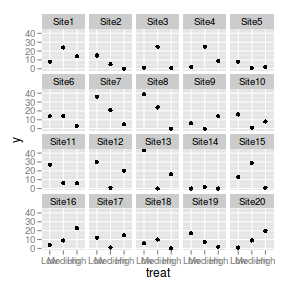
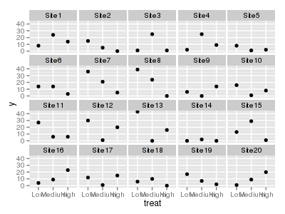
> ggplot(data.hnb, aes(y = y, x = treat)) + geom_point() + facet_wrap(~sites)
> write.table(data.hnb, file = "../downloads/data/data.hnb.csv", quote = F, row.names = F,
+     sep = ",")
Exploratory data analysis and initial assumption checking
Confirm non-normality and explore clumping
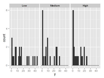
When counts are all very large (not close to 0) and their ranges do not span orders of magnitude, they take on very Gaussian-like properties (symmetrical distribution and variance independent of the mean). Given that models based on the Gaussian distribution are more optimized and recognized than Generalized Linear Mixed Effects Models (GLMM), it can be prudent to adopt Gaussian models for such data. Hence it is a good idea to first explore whether a Poisson model is likely to be more appropriate than a standard Gaussian model.
The potential for overdispersion can be explored by adding a rug to boxplot. The rug is simply tick marks on the inside of an axis at the position corresponding to an observation. As multiple identical values result in tick marks drawn over one another, it is typically a good idea to apply a slight amount of jitter (random displacement) to the values used by the rug.
There are signs of non-normality that would warrant Poisson models. The rug applied to the boxplots does not indicate a serious degree of clumping and there appears to be few zeros. Thus overdispersion is unlikely to be an issue.> library(ggplot2) > ggplot(data.hnb, aes(x = y)) + geom_histogram() + facet_wrap(~treat)
> ggplot(data.hnb, aes(y = y, x = 1)) + geom_boxplot() + geom_rug(position = "jitter",
+     sides = "l") + facet_grid(~treat)
> ggplot(data.hnb, aes(y = y, x = treat)) + geom_point() + facet_wrap(~sites)
Explore zero inflation
Although we have already established that there are few zeros in the data (and thus overdispersion is unlikely to be an issue), we can also explore this by comparing the number of zeros in the data to the number of zeros that would be expected from a Poisson distribution with a mean equal to the mean count of the data.
In the above, the value under FALSE is the proportion of non-zero values in the data and the value under TRUE is the proportion of zeros in the data. In this example, the observed proportion (> # proportion of 0's in the data > data.tab <- table(data.hnb$y == 0) > data.tab/sum(data.tab)
 FALSE   TRUE
0.8833 0.1167
> # proportion of 0's expected from a Poisson distribution
> mu <- mean(data.hnb$y)
> cnts <- rpois(1000, mu)
> data.tab <- table(cnts == 0)
> data.tab/sum(data.tab)
FALSE 1%) corresponds closely to the very low proportion expected (Error in table(data.nb$y == 0) : object 'data.nb' not found
NA%).Model fitting or statistical analysis
> # PQL
> library(MASS)
> a <- glm.nb(y ~ treat, data = data.hnb)
> theta <- a$theta
> data.hnb.glmmPQL <- glmmPQL(y ~ treat, random = list(~1 | sites), data = data.hnb,
+     family = negative.binomial(theta))
>
> # Laplace
> library(lme4)
> data.hnb.glmerL <- glmer(y ~ treat + (1 | sites), data = data.hnb, family = negative.binomial(theta))
> # ADMB
> library(glmmADMB)
> data.hnb.admb <- glmmadmb(y ~ treat + (1 | sites), data = data.hnb, family = "nbinom")
Expected values > 5
Conclusions: the expected values are all greater than 5 and thus PQL is likely to yield reasonably good approximations.> # from PQL > predict(data.hnb.glmmPQL, newdata = data.frame(treat = gl(3, 1, 3, c("Low", "Medium", + "High"))), type = "response", level = 0)
[1] 14.90 10.70  7.95
attr(,"label")
[1] "Predicted values"
> # from Laplace
> predict(data.hnb.glmerL, newdata = data.frame(treat = gl(3, 1, 3, c("Low", "Medium",
+     "High"))), REform = NA, type = "response")
    1     2     3
14.90 10.70  7.95
> # from Laplace
> predict(data.hnb.admb, newdata = data.frame(treat = gl(3, 1, 3, c("Low", "Medium",
+     "High"))), REform = NA, type = "response")
[1] 14.90 10.70 7.95
Lets explore the diagnostics - particularly the residuals
Conclusions: there are no immediately obvious patterns in the residuals. All three approximation techniques yield very similar residuals.> plot(data.hnb.glmmPQL)
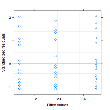
> plot(residuals(data.hnb.glmmPQL, type = "pearson") ~ predict(data.hnb.glmmPQL, type = "link"))

> plot(residuals(data.hnb.glmmPQL, type = "pearson") ~ as.numeric(data.hnb$treat))

>
> # Laplace plot(data.hnb.glmerL)
> plot(residuals(data.hnb.glmerL, type = "pearson") ~ predict(data.hnb.glmerL, type = "link"))

> plot(residuals(data.hnb.glmerL, type = "pearson") ~ as.numeric(data.hnb$treat))

Exploring the model parameters, test hypotheses
> summary(data.hnb.glmmPQL)
Linear mixed-effects model fit by maximum likelihood
 Data: data.hnb
  AIC BIC logLik
   NA  NA     NA

Random effects:
 Formula: ~1 | sites
        (Intercept) Residual
StdDev:   3.657e-05   0.8249

Variance function:
 Structure: fixed weights
 Formula: ~invwt
Fixed effects: y ~ treat
              Value Std.Error DF t-value p-value
(Intercept)  2.7014    0.2084 38  12.963  0.0000
treatMedium -0.3311    0.2963 38  -1.117  0.2708
treatHigh   -0.6282    0.2983 38  -2.106  0.0419
 Correlation:
            (Intr) trtMdm
treatMedium -0.703
treatHigh   -0.699  0.491

Standardized Within-Group Residuals:
    Min      Q1     Med      Q3     Max
-1.1009 -0.9399 -0.2390  0.9089  2.0761

Number of Observations: 60
Number of Groups: 20
> library(aod) > wald.test(b=fixef(data.hnb.glmmPQL), + Sigma=vcov(data.hnb.glmmPQL),Terms=2:3)
Wald test:
----------

Chi-squared test:
X2 = 4.7, df = 2, P(> X2) = 0.096
> intervals(data.hnb.glmmPQL)
Error: cannot get confidence intervals on var-cov
components: Non-positive definite approximate
variance-covariance
> library(gmodels)
> ci(data.hnb.glmmPQL)
            Estimate CI lower CI upper Std. Error
(Intercept)   2.7014    2.279  3.12324     0.2084
treatMedium  -0.3311   -0.931  0.26874     0.2963
treatHigh    -0.6282   -1.232 -0.02439     0.2983
            DF   p-value
(Intercept) 38 1.593e-15
treatMedium 38 2.708e-01
treatHigh   38 4.185e-02
> VarCorr(data.hnb.glmmPQL)
sites = pdLogChol(1)
            Variance  StdDev
(Intercept) 1.337e-09 3.657e-05
Residual    6.805e-01 8.249e-01
> summary(data.hnb.glmerL)
Generalized linear mixed model fit by maximum likelihood ['glmerMod']
 Family: Negative Binomial(0.873) ( log )
Formula: y ~ treat + (1 | sites)
   Data: data.hnb

     AIC      BIC   logLik deviance
   420.9    431.3   -205.4    410.9

Random effects:
 Groups   Name        Variance Std.Dev.
 sites    (Intercept) 0.000    0.000
 Residual             0.681    0.825
Number of obs: 60, groups: sites, 20

Fixed effects:
            Estimate Std. Error t value Pr(>|z|)
(Intercept)    2.701      0.203   13.30   <2e-16
treatMedium   -0.331      0.289   -1.15    0.252
treatHigh     -0.628      0.291   -2.16    0.031

(Intercept) ***
treatMedium
treatHigh   *
---
Signif. codes:
0 '***' 0.001 '**' 0.01 '*' 0.05 '.' 0.1 ' ' 1

Correlation of Fixed Effects:
            (Intr) trtMdm
treatMedium -0.703
treatHigh   -0.699  0.491
> library(aod) > wald.test(b=fixef(data.hnb.glmerL), + Sigma=vcov(data.hnb.glmerL),Terms=2:3)
Wald test:
----------

Chi-squared test:
X2 = 4.7, df = 2, P(> X2) = 0.096
> anova(data.hnb.glmerL)
Analysis of Variance Table
      Df Sum Sq Mean Sq F value
treat  2   3.18    1.59    2.34
> confint(data.hnb.glmerL)
Error: can't (yet) profile GLMMs with non-fixed
scale parameters
> VarCorr(data.hnb.glmerL)
 Groups   Name        Std.Dev.
 sites    (Intercept) 0.000
 Residual             0.825
> summary(data.hnb.admb)
Call:
glmmadmb(formula = y ~ treat + (1 | sites), data = data.hnb,
    family = "nbinom")


Coefficients:
            Estimate Std. Error z value Pr(>|z|)
(Intercept)    2.701      0.246   10.97   <2e-16
treatMedium   -0.331      0.350   -0.95    0.344
treatHigh     -0.628      0.352   -1.78    0.075

(Intercept) ***
treatMedium
treatHigh   .
---
Signif. codes:
0 '***' 0.001 '**' 0.01 '*' 0.05 '.' 0.1 ' ' 1

Number of observations: total=60, sites=20
Random effect variance(s):
Group=sites
             Variance    StdDev
(Intercept) 2.141e-07 0.0004627
Negative binomial dispersion parameter: 0.8745 (std. err.: 0.1764)

Log-likelihood: -205.4
> library(aod) > wald.test(b=fixef(data.hnb.admb), + Sigma=vcov(data.hnb.admb),Terms=2:3)
Wald test:
----------

Chi-squared test:
X2 = 4.1, df = 2, P(> X2) = 0.13
> anova(data.hnb.admb)
Error: Two or more model fits required.
> confint(data.hnb.admb)
             2.5 %  97.5 %
(Intercept)  2.219 3.18395
treatMedium -1.017 0.35507
treatHigh   -1.319 0.06252
> VarCorr(data.hnb.admb)
Group=sites
             Variance    StdDev
(Intercept) 2.141e-07 0.0004627
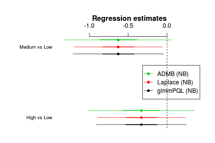
> #install.packages("coefplot2",repos="http://www.math.mcmaster.ca/bolker/R") > library(coefplot2) > > coefplot2(list('glmmPQL (NB)'=data.hnb.glmmPQL, 'Laplace (NB)'=data.hnb.glmerL, 'ADMB (NB)'=data.hnb.admb), varnames=c('High vs Low', 'Medium vs Low'),legend=TRUE,legend.x='right')
Zero-inflation Poisson (ZIP) regression
Scenario and Data
Lets say we wanted to model the abundance of an item ($y$) against a continuous predictor ($x$). As this section is mainly about the generation of artificial data (and not specifically about what to do with the data), understanding the actual details are optional and can be safely skipped. Consequently, I have folded (toggled) this section away.
Random data incorporating the following trends (effect parameters)- the sample size = 20
- the continuous $x$ variable is a random uniform spread of measurements between 1 and 20
- the rate of change in log $y$ per unit of $x$ (slope) = 0.1.
- the value of $x$ when log$y$ equals 0 (when $y$=1)
- to generate the values of $y$ expected at each $x$ value, we evaluate the linear predictor (created by calculating the outer product of the model matrix and the regression parameters). These expected values are then transformed into a scale mapped by (0,$\infty$) by using the log function $e^{linear~predictor}$
- finally, we generate $y$ values by using the expected $y$ values ($\lambda$) as probabilities when drawing random numbers from a Poisson distribution. This step adds random noise to the expected $y$ values and returns only 0's and positive integers.
> set.seed(123)  #3 #7
> # number of sites
> n.sites <- 20
> n.treat <- 3
> n <- n.sites * n.treat
> sites <- gl(n = n.sites, k = n.treat, lab = paste("Site",
+     1:n.sites, sep = ""))
> treat <- gl(n = n.treat, 1, n, lab = c("Low", "Medium",
+     "High"))
> # Xmat <- model.matrix(~sites*treat-1-treat)
> Xmat <- model.matrix(~-1 + sites + treat)
>
> intercept.mean <- 10  # mu alpha
> intercept.sd <- 5  # sigma alpha
> # effect.sd <- 1
> treatM.effect <- -2
> treatH.effect <- -4
> intercept.effects <- rnorm(n = n.sites, mean = intercept.mean,
+     sd = intercept.sd)
> # treatM.effects <- rnorm(n=n.sites,
> # mean=treatM.effect, sd=effect.sd) treatH.effects
> # <- rnorm(n=n.sites, mean=treatH.effect,
> # sd=effect.sd)
> all.effects <- c(intercept.effects, treatM.effect,
+     treatH.effect)  # Put them all together
> lin.pred <- Xmat[, ] %*% all.effects
> lin.pred[lin.pred < 0] <- exp(lin.pred[lin.pred < 0])
> # eps <- rpois(n=n, n.treat) Add some noise and
> # make binomial
> library(gamlss.dist)
> # fixed latent binomial
> y <- rZIP(n, lin.pred, 0.4)
> data.hzip <- data.frame(y, treat, sites)
> head(data.hzip)
  y  treat sites
1 0    Low Site1
2 1 Medium Site1
3 0   High Site1
4 0    Low Site2
5 0 Medium Site2
6 0   High Site2
> write.table(data.hzip, file = "../downloads/data/data.hzip.csv",
+     quote = F, row.names = F, sep = ",")
Exploratory data analysis and initial assumption checking
Confirm non-normality and explore clumping
When counts are all very large (not close to 0) and their ranges do not span orders of magnitude, they take on very Gaussian-like properties (symmetrical distribution and variance independent of the mean). Given that models based on the Gaussian distribution are more optimized and recognized than Generalized Linear Mixed Effects Models (GLMM), it can be prudent to adopt Gaussian models for such data. Hence it is a good idea to first explore whether a Poisson model is likely to be more appropriate than a standard Gaussian model.
The potential for overdispersion can be explored by adding a rug to boxplot. The rug is simply tick marks on the inside of an axis at the position corresponding to an observation. As multiple identical values result in tick marks drawn over one another, it is typically a good idea to apply a slight amount of jitter (random displacement) to the values used by the rug.
There are signs of non-normality that would warrant Poisson models. The rug applied to the boxplots does not indicate a serious degree of clumping and there appears to be few zeros. Thus overdispersion is unlikely to be an issue.> library(ggplot2) > ggplot(data.hzip, aes(x = y)) + geom_histogram() + + facet_wrap(~treat)
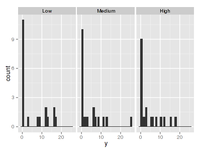
> ggplot(data.hzip, aes(y = y, x = 1)) + geom_boxplot() +
+     geom_rug(position = "jitter", sides = "l") + facet_grid(~treat)
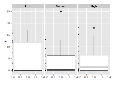
> ggplot(data.hzip, aes(y = y, x = treat)) + geom_point() +
+     facet_wrap(~sites)
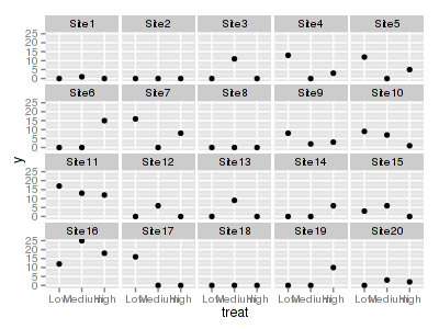
Explore zero inflation
Although we have already established that there are few zeros in the data (and thus overdispersion is unlikely to be an issue), we can also explore this by comparing the number of zeros in the data to the number of zeros that would be expected from a Poisson distribution with a mean equal to the mean count of the data.
In the above, the value under FALSE is the proportion of non-zero values in the data and the value under TRUE is the proportion of zeros in the data. In this example, the observed proportion (> # proportion of 0's in the data > data.tab <- table(data.hzip$y == 0) > data.tab/sum(data.tab)
FALSE  TRUE
  0.5   0.5
> # proportion of 0's expected from a Poisson
> # distribution
> mu <- mean(data.hzip$y)
> cnts <- rpois(1000, mu)
> data.tab <- table(cnts == 0)
> data.tab/sum(data.tab)
FALSE  TRUE
0.988 0.012
50%) corresponds closely to the very low proportion expected (NA, NA%).Model fitting or statistical analysis
> # ADMB ZIP
> library(glmmADMB)
> data.hzip.zip <- glmmadmb(y ~ treat + (1 | sites),
+     data = data.hzip, family = "poisson", zeroInflation = TRUE,
+     admb.opts = admbControl(shess = FALSE, noinit = FALSE))
> # ADMB ZINB
> data.hzip.zinb <- glmmadmb(y ~ treat + (1 | sites),
+     data = data.hzip, family = "nbinom", zeroInflation = TRUE,
+     admb.opts = admbControl(shess = FALSE, noinit = FALSE))
Lets explore
e diagnostics - particularly the residuals Conclusions: there are no immediately obvious patterns in the residuals. All three approximation techniques yield very similar residuals.> plot(resid(data.hzip.zip, type = "pearson") ~ predict(data.hzip.zip, + type = "link"))

> plot(resid(data.hzip.zinb) ~ predict(data.hzip.zinb,
+     type = "link"))

Exploring the model parameters, test hypotheses
> summary(data.hzip.zip)
Call:
glmmadmb(formula = y ~ treat + (1 | sites), data = data.hzip,
    family = "poisson", zeroInflation = TRUE, admb.opts = admbControl(shess = FALSE,
        noinit = FALSE))


Coefficients:
            Estimate Std. Error z value Pr(>|z|)
(Intercept)    0.824      0.160    5.15  2.6e-07
treatMedium    0.312      0.188    1.66    0.097
treatHigh     -0.271      0.173   -1.56    0.118

(Intercept) ***
treatMedium .
treatHigh
---
Signif. codes:
0 '***' 0.001 '**' 0.01 '*' 0.05 '.' 0.1 ' ' 1

Number of observations: total=60, sites=20
Random effect variance(s):
Group=sites
            Variance StdDev
(Intercept)    1.067  1.033
Zero-inflation: 0.4895  (std. err.:  0.06974 )

Log-likelihood: -144.6
> library(aod) > wald.test(b=fixef(data.hzip.zip), + Sigma=vcov(data.hzip.zip),Terms=2:3)
Wald test:
----------

Chi-squared test:
X2 = 20.6, df = 2, P(> X2) = 3.4e-05
> intervals(data.hzip.zip)
Error: no applicable method for 'intervals'
applied to an object of class "glmmadmb"
> library(gmodels)
> ci(data.hzip.zip)
Error: (list) object cannot be coerced to type
'double'
> VarCorr(data.hzip.zip)
Group=sites
            Variance StdDev
(Intercept)    1.067  1.033
> summary(data.hzip.zinb)
Call:
glmmadmb(formula = y ~ treat + (1 | sites), data = data.hzip,
    family = "nbinom", zeroInflation = TRUE, admb.opts = admbControl(shess = FALSE,
        noinit = FALSE))


Coefficients:
            Estimate Std. Error z value Pr(>|z|)
(Intercept)    2.360      0.211   11.20   <2e-16
treatMedium   -0.287      0.249   -1.15    0.250
treatHigh     -0.562      0.222   -2.54    0.011

(Intercept) ***
treatMedium
treatHigh   *
---
Signif. codes:
0 '***' 0.001 '**' 0.01 '*' 0.05 '.' 0.1 ' ' 1

Number of observations: total=60, sites=20
Random effect variance(s):
Group=sites
            Variance StdDev
(Intercept)   0.2491 0.4991
Negative binomial dispersion parameter: 13.45 (std. err.: 13.89)
Zero-inflation: 0.4949  (std. err.:  0.06534 )

Log-likelihood: -130.3
> library(aod) > wald.test(b=fixef(data.hzip.zinb), + Sigma=vcov(data.hzip.zinb),Terms=2:3)
Wald test:
----------

Chi-squared test:
X2 = 8.5, df = 2, P(> X2) = 0.015
> anova(data.hzip.zinb)
Error: Two or more model fits required.
> confint(data.hzip.zinb)
              2.5 %  97.5 %
(Intercept)  1.9467  2.7725
treatMedium -0.7754  0.2018
treatHigh   -0.9967 -0.1278
> VarCorr(data.hzip.zinb)
Group=sites
            Variance StdDev
(Intercept)   0.2491 0.4991
Bonus
> copper <- read.table("../downloads/data/copper.csv",
+     header = T, sep = ",", strip.white = T)
> head(copper)
   COPPER PLATE DIST WORMS
1 control   200    4 11.50
2 control   200    3 13.00
3 control   200    2 13.50
4 control   200    1 12.00
5 control    39    4 17.75
6 control    39    3 13.75
> copper$PLATE <- factor(copper$PLATE)
> copper$DIST <- factor(copper$DIST)
> replications(WORMS ~ COPPER + Error(PLATE) + DIST +
+     COPPER:DIST, data = copper)
     COPPER        DIST COPPER:DIST
         20          15           5
> > copper.lme <- lme(WORMS ~ COPPER * DIST, random = ~1 | + PLATE, data = copper) > copper.lme1 <- lme(WORMS ~ COPPER * DIST, random = ~1 | + PLATE, data = copper, correlation = corCompSymm(form = ~1 | + PLATE)) > copper.lme2 <- lme(WORMS ~ COPPER * DIST, random = ~1 | + PLATE, data = copper, correlation = corAR1(form = ~1 | + PLATE)) > anova(copper.lme, copper.lme1)
            Model df   AIC   BIC logLik   Test
copper.lme      1 14 218.2 244.4 -95.13
copper.lme1     2 15 220.2 248.3 -95.13 1 vs 2
              L.Ratio p-value
copper.lme
copper.lme1 2.274e-13       1
> # Check whether a first order autoregressive > # correlation structure is more appropriate > copper.lme2 <- update(copper.lme, correlation = corAR1(form = ~1 | + PLATE)) > anova(copper.lme, copper.lme2)
            Model df   AIC   BIC logLik   Test
copper.lme      1 14 218.2 244.4 -95.13
copper.lme2     2 15 214.4 242.4 -92.19 1 vs 2
            L.Ratio p-value
copper.lme
copper.lme2   5.881  0.0153
> # Now fit the 'best'' model with REML copper.lme3 > # <-update(copper.lme2, method='REML') > anova.lme(copper.lme2)
            numDF denDF F-value p-value
(Intercept)     1    36   980.6  <.0001
COPPER          2    12    93.1  <.0001
DIST            3    36    25.1  <.0001
COPPER:DIST     6    36     4.3  0.0025
>
>
> library(MASS)
> copper.glmmPQL <- glmmPQL(WORMS ~ COPPER * DIST, random = ~1 |
+     PLATE, data = copper, family = "poisson")
> copper.glmmPQL1 <- update(copper.glmmPQL, correlation = corCompSymm(form = ~1 |
+     PLATE))
> copper.glmmPQL2 <- update(copper.glmmPQL, correlation = corAR1(form = ~1 |
+     PLATE))
>
> plot(residuals(copper.glmmPQL, type = "pearson") ~
+     predict(copper.glmmPQL, type = "link"))

> plot(residuals(copper.glmmPQL, type = "pearson") ~
+     as.numeric(copper$COPPER))

> plot(residuals(copper.glmmPQL, type = "pearson") ~
+     as.numeric(copper$DIST))

>
>
> plot(residuals(copper.glmmPQL2, type = "pearson") ~
+     predict(copper.glmmPQL2, type = "link"))

> plot(residuals(copper.glmmPQL2, type = "pearson") ~
+     as.numeric(copper$COPPER))

> plot(residuals(copper.glmmPQL2, type = "pearson") ~
+     as.numeric(copper$DIST))

>
>
> # cant do anova(..), cant do AIC
>
> # test interaction
> wald.test(b = fixef(copper.glmmPQL2), Sigma = vcov(copper.glmmPQL2),
+     Terms = 7:12)
Wald test:
----------

Chi-squared test:
X2 = 74.0, df = 6, P(> X2) = 6.1e-14
>
> plot(allEffects(copper.glmmPQL), type = "response")
Error: could not find function "allEffects"
>
> contrasts(copper$DIST) <- contr.poly
> contrasts(copper$COPPER) <- contr.treatment
> bb <- update(copper.glmmPQL2, contrasts = list(DIST = "contr.poly"))
> library(contrast)
> contrast(copper.glmmPQL2, a = list(COPPER == "Week 2",
+     DIST = 1:4), b = list(COPPER == "Week 2", DIST = 1:4))
Error: object 'COPPER' not found
