Tutorial 9.3a - Randomized Complete Block ANOVA
20 Jul 2018
Overview
When single sampling units are selected amongst highly heterogeneous conditions, it is unlikely that these single units will adequately represent the populations and repeated sampling is likely to yield very different outcomes.
Tutorial 9.2a (Nested ANOVA), introduced the concept of employing sub-replicates that are nested within the main treatment levels as a means of absorbing some of the unexplained variability that would otherwise arise from designs in which sampling units are selected from amongst highly heterogeneous conditions. Such (nested) designs are useful in circumstances where the levels of the main treatment (such as burnt and un-burnt sites) occur at a much larger temporal or spatial scale than the experimental/sampling units (e.g. vegetation monitoring quadrats).
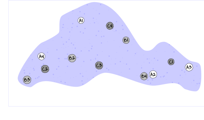
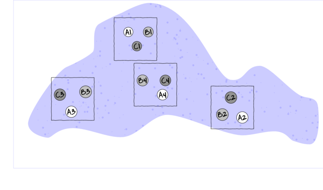
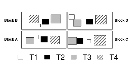
For circumstances in which the main treatments can be applied (or naturally occur) at the same scale as the sampling units (such as whether a stream rock is enclosed by a fish proof fence or not), an alternative design is available. In this design (randomized complete block design), each of the levels of the main treatment factor are grouped (blocked) together (in space and/or time) and therefore, whilst the conditions between the groups (referred to as `blocks') might vary substantially, the conditions under which each of the levels of the treatment are tested within any given block are far more homogeneous (see Figure below).
If any differences between blocks (due to the heterogeneity) can account for some of the total variability between the sampling units (thereby reducing the amount of variability that the main treatment(s) failed to explain), then the main test of treatment effects will be more powerful/sensitive.
As an simple example of a randomized complete block (RCB) design, consider an investigation into the roles of different organism scales (microbial, macro invertebrate and vertebrate) on the breakdown of leaf debris packs within streams. An experiment could consist of four treatment levels - leaf packs protected by fish-proof mesh, leaf packs protected by fine macro invertebrate exclusion mesh, leaf packs protected by dissolving antibacterial tablets, and leaf packs relatively unprotected as controls.
As an acknowledgement that there are many other unmeasured factors that could influence leaf pack breakdown (such as flow velocity, light levels, etc) and that these are likely to vary substantially throughout a stream, the treatments are to be arranged into groups or 'blocks' (each containing a single control, microbial, macro invertebrate and fish protected leaf pack). Blocks of treatment sets are then secured in locations haphazardly selected throughout a particular reach of stream. Importantly, the arrangement of treatments in each block must be randomized to prevent the introduction of some systematic bias - such as light angle, current direction etc.
Blocking does however come at a cost. The blocks absorb both unexplained variability as well as degrees of freedom from the residuals. Consequently, if the amount of the total unexplained variation that is absorbed by the blocks is not sufficiently large enough to offset the reduction in degrees of freedom (which may result from either less than expected heterogeneity, or due to the scale at which the blocks are established being inappropriate to explain much of the variation), for a given number of sampling units (leaf packs), the tests of main treatment effects will suffer power reductions.
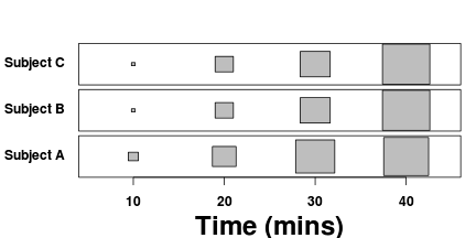
Treatments can also be applied sequentially or repeatedly at the scale of the entire block, such that at any single time, only a single treatment level is being applied (see the lower two sub-figures above). Such designs are called repeated measures. A repeated measures ANOVA is to an single factor ANOVA as a paired t-test is to a independent samples t-test.
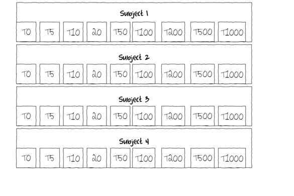
One example of a repeated measures analysis might be an investigation into the effects of a five different diet drugs (four doses and a placebo) on the food intake of lab rats. Each of the rats (`subjects') is subject to each of the four drugs (within subject effects) which are administered in a random order.
In another example, temporal recovery responses of sharks to bi-catch entanglement stresses might be simulated by analyzing blood samples collected from captive sharks (subjects) every half hour for three hours following a stress inducing restraint. This repeated measures design allows the anticipated variability in stress tolerances between individual sharks to be accounted for in the analysis (so as to permit more powerful test of the main treatments). Furthermore, by performing repeated measures on the same subjects, repeated measures designs reduce the number of subjects required for the investigation.
Essentially, this is a randomized complete block design except that the within subject (block) effect (e.g. time since stress exposure) cannot be randomized (the consequences of which are discussed in section on Sphericity).
To suppress contamination effects resulting from the proximity of treatment sampling units within a block, units should be adequately spaced in time and space. For example, the leaf packs should not be so close to one another that the control packs are effected by the antibacterial tablets and there should be sufficient recovery time between subsequent drug administrations.
In addition, the order or arrangement of treatments within the blocks must be randomized so as to prevent both confounding as well as computational complications (Sphericity). Whilst this is relatively straight forward for the classic randomized complete block design (such as the leaf packs in streams), it is logically not possible for repeated measures designs.
Blocking factors are typically random factors (see section~\ref{chpt:ANOVA.fixedVsRandomFactor}) that represent all the possible blocks that could be selected. As such, no individual block can truly be replicated. Randomized complete block and repeated measures designs can therefore also be thought of as un-replicated factorial designs in which there are two or more factors but that the interactions between the blocks and all the within block factors are not replicated.
Linear models
The linear models for two and three factor nested design are:
$$
\begin{align}
y_{ij}&=\mu+\beta_{i}+\alpha_j + \varepsilon_{ij} &\hspace{2em} \varepsilon_{ij} &\sim\mathcal{N}(0,\sigma^2), \hspace{1em}\sum{}{\beta=0}\\
y_{ijk}&=\mu+\beta_{i} + \alpha_j + \gamma_{k} + \beta\alpha_{ij} + \beta\gamma_{ik} + \alpha\gamma_{jk} + \gamma\alpha\beta_{ijk} + \varepsilon_{ijk} \hspace{2em} (Model 1)\\
y_{ijk}&=\mu+\beta_{i} + \alpha_j + \gamma_{k} + \alpha\gamma_{jk} + \varepsilon_{ijk} \hspace{2em}(Model 2)
\end{align}
$$
where $\mu$ is the overall mean, $\beta$ is the effect of the Blocking
Factor B, $\alpha$ and $\gamma$ are the effects of withing block Factor A
and Factor C respectively and $\varepsilon$ is the random unexplained or
residual component.
Tests for the effects of blocks as well as effects within blocks assume that there are no interactions between blocks and the within block effects. That is, it is assumed that any effects are of similar nature within each of the blocks. Whilst this assumption may well hold for experiments that are able to consciously set the scale over which the blocking units are arranged, when designs utilize arbitrary or naturally occurring blocking units, the magnitude and even polarity of the main effects are likely to vary substantially between the blocks.
The preferred (non-additive or `Model 1') approach to un-replicated factorial analysis of some bio-statisticians is to include the block by within subject effect interactions (e.g. $\beta\alpha$). Whilst these interaction effects cannot be formally tested, they can be used as the denominators in F-ratio calculations of their respective main effects tests (see the tables that follow).
Proponents argue that since these blocking interactions cannot be formally tested, there is no sound inferential basis for using these error terms separately. Alternatively, models can be fitted additively (`Model 2') whereby all the block by within subject effect interactions are pooled into a single residual term ($\varepsilon$). Although the latter approach is simpler, each of the within subject effects tests do assume that there are no interactions involving the blocks and that perhaps even more restrictively, that sphericity (see section Sphericity) holds across the entire design.
Null hypotheses
Separate null hypotheses are associated with each of the factors, however, blocking factors are typically only added to absorb some of the unexplained variability and therefore specific hypothesis tests associated with blocking factors are of lesser biological importance.
Factor A - the main within block treatment effect
Fixed (typical case)
H$_0(A)$: $\mu_1=\mu_2=...=\mu_i=\mu$ (the population group means of A (pooling B) are all equal)
The mean of population 1 (pooling blocks) is equal to that of population 2 and so on, and thus all population means are equal to an overall mean.
No effect of A within each block (Model 2) or over and above the effect of blocks.
If the effect of the $i^{th}$ group is the difference between the $i^{th}$ group mean and the overall mean ($\alpha_i = \mu_i - \mu$) then the H$_0$ can alternatively be written as:
H$_0(A)$: $\alpha_1 = \alpha_2 = ... = \alpha_i = 0$ (the effect of each group equals zero)
If one or more of the $\alpha_i$ are different from zero (the response mean for this treatment differs from the overall response mean), the null hypothesis is not true indicating that the treatment does affect the response variable.
Random
H$_0(A)$: $\sigma_\alpha^2=0$ (population variance equals zero)
There is no added variance due to all possible levels of A (pooling B).
Factor B - the blocking factor
Random (typical case)
H$_0(B)$: $\sigma_\beta^2=0$ (population variance equals zero)
There is no added variance due to all possible levels of B.
Fixed
H$_0(B)$: $\mu_{1}=\mu_{2}=...=\mu_{i}=\mu$ (the population group means of B are all equal)
H$_0(B)$: $\beta_{1} = \beta_{2}= ... = \beta_{i} = 0$ (the effect of each chosen B group equals zero)
The null hypotheses associated with additional within block factors, are treated similarly to Factor A above.
Analysis of Variance
Partitioning of the total variance sequentially into explained and unexplained components and F-ratio calculations predominantly follows the rules established in tutorials on Nested ANOVA and Factorial ANOVA. Randomized block and repeated measures designs can essentially be analysed as Model III ANOVAs. The appropriate unexplained residuals and therefore the appropriate F-ratios for each factor differ according to the different null hypotheses associated with different combinations of fixed and random factors and what analysis approach (Model 1 or 2) is adopted for the randomized block linear model (see the following tables).
In additively (Model 2) fitted models (in which block interactions are assumed not to exist and are thus pooled into a single residual term), hypothesis tests of the effect of B (blocking factor) are possible. However, since blocking designs are usually employed out of expectation for substantial variability between blocks, such tests are rarely of much biological interest.
| F-ratio | ||||||
|---|---|---|---|---|---|---|
| Factor | d.f | MS | Model 1 (non-additive) | Model 2 (additive) | ||
| B$^\prime$ (block) | $b-1$ | $MS_{B^\prime}$ | $\large\frac{MS_{B^\prime}}{MS_{Resid}}$ | $\large\frac{MS_{B^\prime}}{MS_{Resid}}$ | ||
| A | $a-1$ | $MS_A$ | $\large\frac{MS_A}{MS_{Resid}}$ | $\large\frac{MS_A}{MS_{Resid}}$ | ||
| Residual (=B$^\prime$A)) | $(b-1)(a-1)$ | $MS_{Resid}$ | ||||
| R syntax | ||||||
| Balanced |
summary(aov(y~A+Error(B), data)) |
|||||
| Balanced or unbalanced |
library(nlme) summary(lme(y~A, random=~1|B, data)) anova(lme(y~A, random=~1|B, data)) #OR library(lme4) summary(lmer(y~(1|B)+A, data)) |
|||||
| Variance components |
library(nlme) summary(lme(y~1, random=~1|B/A, data)) #OR library(lme4) summary(lmer(y~(1|B)+(1|A), data)) |
|||||
| F-ratio | ||||||||
|---|---|---|---|---|---|---|---|---|
| A&C fixed, B random | A fixed, B&C random | A,B&C random | ||||||
| Factor | d.f. | Model 1 | Model 2 | Model 1 | Model 2 | Model 1 | Model 2 | |
| 1 | B | $b-1$ | $1/7$ | $1/7$ | $1/6$ | $1/7$ | $1/(5+6-7)$ | $1/7$ |
| 2 | A | $a-1$ | $2/5$ | $2/7$ | $2/(4+5-7)$ | $2/4$ | $2/(4+5-7)$ | $1/4$ |
| 3 | C | $c-1$ | $3/6$ | $3/7$ | $3/6$ | $3/7$ | $3/(4+6-7)$ | $3/4$ |
| 4 | A$\times$C | $(a-1)(c-1)$ | $4/7$ | $4/7$ | $4/7$ | $4/7$ | $4/7$ | $4/7$ |
| 5 | B${^\prime}\times$A | $(b-1)(a-1)$ | No test | No test | $5/7$ | |||
| 6 | B${^\prime}\times$C | $(b-1)(c-1)$ | No test | No test | $6/7$ | |||
| 7 | Residuals (=B$^{\prime}\times$A$\times$C) | $(b-1)(a-1)(c-1)$ | ||||||
| B random, A&C fixed | ||||||||
| Model 1 |
summary(aov(y~Error(B/(A*C))+A*C, data)) |
|||||||
| Model 2 |
summary(aov(y~Error(B)+A*C, data)) #or library(nlme) summary(lme(y~A*C, random=~1|B, data)) |
|||||||
| Unbalanced |
anova(lme(DV~A*C, random=~1|B), type='marginal') anova(lme(DV~A*C, random=~1|B, correlation=corAR1(form=~1|B)), type='marginal') |
|||||||
| Other models | ||||||||
library(lmer) summary(lmer(DV~(~1|A*C)+(1|B)), data) #for example # or summary(lm(y~A*B*C, data)) # and make manual F-ratio etc adjustments |
||||||||
| Variance components |
library(nlme) summary(lme(y~1, random=~1|B/(A*C), data)) |
|||||||
Assumptions
As with other ANOVA designs, the reliability of hypothesis tests is dependent on the residuals being:
- normally distributed. Boxplots using the appropriate scale of replication (reflecting the appropriate residuals/F-ratio denominator (see Tables above) should be used to explore normality. Scale transformations are often useful.
- equally varied. Boxplots and plots of means against variance (using the appropriate scale of replication) should be used to explore the spread of values. Residual plots should reveal no patterns. Scale transformations are often useful.
- independent of one another. Although the observations within a block may not strictly be independent, provided the treatments are applied or ordered randomly within each block or subject, within block proximity effects on the residuals should be random across all blocks and thus the residuals should still be independent of one another. Nevertheless, it is important that experimental units within blocks are adequately spaced in space and time so as to suppress contamination or carryover effects.
Sphericity
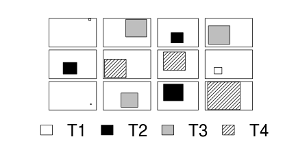
Un-replicated factorial designs extend the usual equal variance (no relationship between mean and variance) assumption to further assume that the differences between each pair of within block treatments are equally varied across the blocks (see the following figure). To meet this assumption a matrix of variances (between pairs of observations within treatments) and covariances (between treatment pairs within each block) must display a pattern known as sphericity. Strickly, the variance-covariance matrix must display a very specific pattern of sphericity in which both variances and covariances are equal (compound symmetry), however an F-ratio will still reliably follow an F distribution provided basic sphericity holds.
| Single factor ANOVA | |||||||||||||||||||||||||||
|---|---|---|---|---|---|---|---|---|---|---|---|---|---|---|---|---|---|---|---|---|---|---|---|---|---|---|---|
|
Variance-covariance structure
|
||||||||||||||||||||||||||
| Randomized Complete Block | |||||||||||||||||||||||||||
|
Variance-covariance structure
|
||||||||||||||||||||||||||
| Repeated Measures Design | |||||||||||||||||||||||||||
|
Variance-covariance structure
|
||||||||||||||||||||||||||
Typically, un-replicated factorial designs in which the treatment levels have been randomly arranged (temporally and spatially) within each block (randomized complete block) should meet this sphericity assumption. Conversely, repeated measures designs that incorporate factors whose levels cannot be randomized within each block (such as distances from a source or time), are likely to violate this assumption. In such designs, the differences between treatments that are arranged closer together (in either space or time) are likely to be less variable (greater paired covariances) than the differences between treatments that are further apart.
Hypothesis tests are not very robust to substantial deviations from sphericity and consequently tend to have inflated type I errors. There are three broad techniques for compensating or tackling the issues of sphericity:
- reducing the degrees of freedom for F tests according to the degree of departure from sphericity (measured by epsilon ($\epsilon$)). The two main estimates of epsilon are Greenhouse-Geisser and Huynh-Feldt, the former of which is preferred (as it provides more liberal protection) unless its value is less than 0.5.
- perform a multivariate ANOVA (MANOVA). Although the sphericity assumption does not apply to such procedures, MANOVA's essentially test null hypotheses about the differences between multiple treatment pairs (and thus test whether an array of population means equals zero), and therefore assume multivariate normality - a difficult assumption to explore.
- fit a linear mixed effects (lme) model and incorporate a particular correlation structure into the modelling. The approximate form of the correlation structure can be specified up-front when fitting linear mixed effects models (via lme) and thus correlated data are more appropriately handled. A selection of variance-covariance structures appropriate for biological data are listed in Table~\ref{tab:randomizedBlockAnova-correlationStructures}. It is generally recommended that linear mixed effects models be fitted with a range of covariance structures. The "best" covariance structure is that the results in a better fit (as measured by either AIC, BIC or ANOVA) than a model fitted with a compound symmetry structure.
Block by treatment interactions
The presence of block by treatment interactions have important implications for models that incorporate a single within block factor as well as additive models involving two or more within block factors. In both cases, the blocking interactions and overall random errors are pooled into a residual term that is used as the denominator in F-ratio calculations (see the tables above).
Consequently, block by treatment interactions increase the denominator ($MS_{Resid}$) resulting in lower F-ratios (lower power). Moreover, the presence of strong blocking interactions would imply that any effects of the main factor are not consistent. Drawing conclusions from such an analysis (particularly in light of non-significant main effects) is difficult. Unless we assume that there are no block by within block interactions, non-significant within block effects could be due to either an absence of a treatment effect, or as a result of opposing effects within different blocks. As these block by within block interactions are unreplicated, they can neither be formally tested nor is it possible to perform main effects tests to diagnose non-significant within block effects.
Block by treatment interactions can be diagnosed by examining;
- interaction (cell means) plot. The mean ($n=1$) response for each level of the main factor is plotted against the block number. Parallel lines infer no block by treatment interaction.
- residual plot. A curvilinear pattern in which the residual values switch from positive to negative and back again (or visa versa) over the range of predicted values implies that the scale (magnitude but not polarity) of the main treatment effects differs substantially across the range of blocks. Scale transformations can be useful in removing such interactions.
- Tukey's test for non-additivity evaluated at $\alpha=0.10$ or even $\alpha=0.25$. This (curvilinear test) formally tests for the presence of a quadratic trend in the relationship between residuals and predicted values. As such, it too is only appropriate for simple interactions of scale.
$R^2$ approximations
Whilst $R^2$ is a popular goodness of fit metric in simple linear models, its use is rarely extended to (generalized) linear mixed effects models. The reasons for this include:
- there are numerous ways that $R^2$ could be defined for mixed effects models, some of which can result in values that are either difficult to interpret or illogical (for example negative $R^2$).
- perhaps as a consequence, software implementation is also largely lacking.
Nakagawa and Schielzeth (2013) discuss the issues associated with $R^2$ calculations and
suggest a series of simple calculations to yield sensible $R^2$ values from mixed effects models.
An $R^2$ value quantifies the proportion of variance explained by a model (or by terms in a model) - the higher the
value, the better the model (or term) fit.
Nakagawa and Schielzeth (2013) offered up two $R^2$ for mixed effects models:
- Marginal $R^2$ - the proportion of total variance explained by the fixed effects. $$ \text{Marginal}~R^2 = \frac{\sigma^2_f}{\sigma^2_f + \sum^z_l{\sigma^2_l} + \sigma^2_d + \sigma^2_e} $$ where $\sigma^2_f$ is the variance of the fitted values (i.e. $\sigma^2_f = var(\mathbf{X\beta})$) on the link scale, $\sum^z_l{\sigma^2_l}$ is the sum of the $z$ random effects (including the residuals) and $\sigma^2_d$ and $\sigma^2_e$ are additional variance components appropriate when using non-Gaussian distributions.
- Conditional $R^2$ - the proportion of the total variance collectively explained by the fixed and random factors $$ \text{Conditional}~R^2 = \frac{\sigma^2_f + \sum^z_l{\sigma^2_l}}{\sigma^2_f + \sum^z_l{\sigma^2_l} + \sigma^2_d + \sigma^2_e} $$
ANOVA in R
Simple RCB
Scenario and Data
Imagine we has designed an experiment in which we intend to measure a response ($y$) to one of treatments (three levels; 'a1', 'a2' and 'a3'). Unfortunately, the system that we intend to sample is spatially heterogeneous and thus will add a great deal of noise to the data that will make it difficult to detect a signal (impact of treatment).
Thus in an attempt to constrain this variability you decide to apply a design (RCB) in which each of the treatments within each of 35 blocks dispersed randomly throughout the landscape. As this section is mainly about the generation of artificial data (and not specifically about what to do with the data), understanding the actual details are optional and can be safely skipped. Consequently, I have folded (toggled) this section away.
- the number of treatments = 3
- the number of blocks containing treatments = 35
- the mean of the treatments = 40, 70 and 80 respectively
- the variability (standard deviation) between blocks of the same treatment = 12
- the variability (standard deviation) between treatments withing blocks = 5
library(plyr)
set.seed(1)
nTreat <- 3
nBlock <- 35
sigma <- 5
sigma.block <- 12
n <- nBlock * nTreat
Block <- gl(nBlock, k = 1)
A <- gl(nTreat, k = 1, lab = LETTERS[1:nTreat])
dt <- expand.grid(A = A, Block = Block)
# Xmat <- model.matrix(~Block + A + Block:A, data=dt)
Xmat <- model.matrix(~-1 + Block + A, data = dt)
block.effects <- rnorm(n = nBlock, mean = 40, sd = sigma.block)
A.effects <- c(30, 40)
all.effects <- c(block.effects, A.effects)
lin.pred <- Xmat %*% all.effects

# OR
Xmat <- cbind(model.matrix(~-1 + Block, data = dt), model.matrix(~-1 + A, data = dt))
## Sum to zero block effects
block.effects <- rnorm(n = nBlock, mean = 0, sd = sigma.block)
A.effects <- c(40, 70, 80)
all.effects <- c(block.effects, A.effects)
lin.pred <- Xmat %*% all.effects


## the quadrat observations (within sites) are drawn from normal distributions with means according to
## the site means and standard deviations of 5
y <- rnorm(n, lin.pred, sigma)
data.rcb1 <- data.frame(y = y, expand.grid(A = A, Block = paste0("B", Block)))
head(data.rcb1)  #print out the first six rows of the data set
         y A Block
1 37.39761 A    B1
2 61.47033 B    B1
3 78.07370 C    B1
4 30.59803 A    B2
5 59.00035 B    B2
6 76.72575 C    B2
write.table(data.rcb1, file = "../downloads/data/data.rcb1.csv", quote = FALSE, row.names = FALSE, sep = ",")
Exploratory data analysis
Normality and Homogeneity of variance
boxplot(y ~ A, data.rcb1)

Conclusions:
- there is no evidence that the response variable is consistently non-normal across all populations - each boxplot is approximately symmetrical
- there is no evidence that variance (as estimated by the height of the boxplots) differs between the five populations. . More importantly, there is no evidence of a relationship between mean and variance - the height of boxplots does not increase with increasing position along the y-axis. Hence it there is no evidence of non-homogeneity
- transform the scale of the response variables (to address normality etc). Note transformations should be applied to the entire response variable (not just those populations that are skewed).
Block by within-Block interaction
library(car)
with(data.rcb1, interaction.plot(A, Block, y))

# OR with ggplot
library(ggplot2)
ggplot(data.rcb1, aes(y = y, x = A, group = Block, color = Block)) +
    geom_line() + guides(color = guide_legend(ncol = 3))

library(car)
residualPlots(lm(y ~ Block + A, data.rcb1))

           Test stat Pr(>|t|)
Block             NA       NA
A                 NA       NA
Tukey test    -0.885    0.376
# the Tukey's non-additivity test by itself can be obtained via an
# internal function within the car package
car:::tukeyNonaddTest(lm(y ~ Block + A, data.rcb1))
      Test     Pvalue
-0.8854414  0.3759186
# alternatively, there is also a Tukey's non-additivity test
# within the asbio package
library(asbio)
with(data.rcb1, tukey.add.test(y, A, Block))
Tukey's one df test for additivity
F = 0.7840065   Denom df = 67    p-value = 0.3790855
Conclusions:
- there is no visual or inferential evidence of any major interactions between Block and the within-Block effect (A). Any trends appear to be reasonably consistent between Blocks.
Model fitting or statistical analysis
There are numerous ways of fitting a nested ANOVA in R.
Linear mixed effects modelling via the lme() function. This method is one of the original implementations in which separate variance-covariance matrices are incorporated into a interactive sequence of (generalized least squares) and maximum likelihood (actually REML) estimates of 'fixed' and 'random effects'.
Rather than fit just a single, simple random intercepts model, it is common to fit other related alternative models and explore which model fits the data best. For example, we could also fit a random intercepts and slope model. We could also explore other variance-covariance structures (autocorrelation or heterogeneity).
library(nlme)
# random intercept
data.rcb1.lme <- lme(y ~ A, random = ~1 | Block, data.rcb1, method = "REML")
# random intercept/slope
data.rcb1.lme1 <- lme(y ~ A, random = ~A | Block, data.rcb1, method = "REML")
anova(data.rcb1.lme, data.rcb1.lme1)
               Model df      AIC      BIC    logLik   Test  L.Ratio p-value
data.rcb1.lme      1  5 722.1087 735.2336 -356.0544
data.rcb1.lme1     2 10 727.2001 753.4499 -353.6001 1 vs 2 4.908574  0.4271
More modern linear mixed effects modelling via the lmer() function. In contrast to the lme() function, the lmer() function supports are more complex combination of random effects (such as crossed random effects). However, unfortunately, it does not yet (and probably never will) have a mechanism to support specifying alternative covariance structures needed to accommodate spatial and temporal autocorrelation
library(lme4)
data.rcb1.lmer <- lmer(y ~ A + (1 | Block), data.rcb1, REML = TRUE)  #random intercept
data.rcb1.lmer1 <- lmer(y ~ A + (A | Block), data.rcb1, REML = TRUE,
    control = lmerControl(check.nobs.vs.nRE = "ignore"))  #random intercept/slope
anova(data.rcb1.lmer, data.rcb1.lmer1)
Data: data.rcb1
Models:
data.rcb1.lmer: y ~ A + (1 | Block)
data.rcb1.lmer1: y ~ A + (A | Block)
                Df    AIC    BIC  logLik deviance  Chisq Chi Df Pr(>Chisq)
data.rcb1.lmer   5 729.03 742.30 -359.51   719.03
data.rcb1.lmer1 10 733.98 760.52 -356.99   713.98 5.0529      5     0.4095
Mixed effects models can also be fit using the Template Model Builder automatic differentiation engine via the glmmTMB() function from a package with the same name. glmmTMB is able to fit similar models to lmer, yet can also incorporate more complex features such as zero inflation and temporal autocorrelation. Random effects are assumed to be Gaussian on the scale of the linear predictor and are integrated out via Laplace approximation. On the downsides, REML is not available for this technique yet and nor is Gauss-Hermite quadrature (which can be useful when dealing with small sample sizes and non-gaussian errors.
library(glmmTMB)
data.rcb1.glmmTMB <- glmmTMB(y ~ A + (1 | Block), data.rcb1)  #random intercept
data.rcb1.glmmTMB1 <- glmmTMB(y ~ A + (A | Block), data.rcb1)  #random intercept/slope
anova(data.rcb1.glmmTMB, data.rcb1.glmmTMB1)
Data: data.rcb1
Models:
data.rcb1.glmmTMB: y ~ A + (1 | Block), zi=~0, disp=~1
data.rcb1.glmmTMB1: y ~ A + (A | Block), zi=~0, disp=~1
                   Df    AIC   BIC  logLik deviance Chisq Chi Df Pr(>Chisq)
data.rcb1.glmmTMB   5 729.03 742.3 -359.51   719.03
data.rcb1.glmmTMB1 10                                          5
Traditional OLS with multiple error strata using the aov() function. The aov() function is actually a wrapper for a specialized lm() call that defines multiple residual terms and thus adds some properties and class attributes to the fitted model that modify the output. This option is illustrated purely as a link to the past, it is no longer considered as robust or flexible as more modern techniques.
data.rcb1.aov <- aov(y ~ A + Error(Block), data.rcb1)
Model evaluation
Residuals
As always, exploring the residuals can reveal issues of heteroscadacity, non-linearity and potential issues with autocorrelation. Note for lme() and lmer() residual plots use standardized (normalized) residuals rather than raw residuals as the former reflect changes to the variance-covariance matrix whereas the later do not.
The following function will be used for the production of some of the qqnormal plots.
qq.line = function(x) {
    # following four lines from base R's qqline()
    y <- quantile(x[!is.na(x)], c(0.25, 0.75))
    x <- qnorm(c(0.25, 0.75))
    slope <- diff(y)/diff(x)
    int <- y[1L] - slope * x[1L]
    return(c(int = int, slope = slope))
}
plot(data.rcb1.lme)

qqnorm(resid(data.rcb1.lme))
qqline(resid(data.rcb1.lme))

library(sjPlot)
plot_grid(plot_model(data.rcb1.lme, type = "diag"))

plot(data.rcb1.lmer)

plot(fitted(data.rcb1.lmer), residuals(data.rcb1.lmer, type = "pearson",
    scaled = TRUE))

ggplot(fortify(data.rcb1.lmer), aes(y = .scresid, x = .fitted)) +
    geom_point()

QQline = qq.line(fortify(data.rcb1.lmer)$.scresid)
ggplot(fortify(data.rcb1.lmer), aes(sample = .scresid)) + stat_qq() +
    geom_abline(intercept = QQline[1], slope = QQline[2])

qqnorm(resid(data.rcb1.lmer))
qqline(resid(data.rcb1.lmer))

library(sjPlot)
plot_grid(plot_model(data.rcb1.lmer, type = "diag"))

ggplot(data = NULL, aes(y = resid(data.rcb1.glmmTMB, type = "pearson"),
    x = fitted(data.rcb1.glmmTMB))) + geom_point()

QQline = qq.line(resid(data.rcb1.glmmTMB, type = "pearson"))
ggplot(data = NULL, aes(sample = resid(data.rcb1.glmmTMB, type = "pearson"))) +
    stat_qq() + geom_abline(intercept = QQline[1], slope = QQline[2])

library(sjPlot)
plot_grid(plot_model(data.rcb1.glmmTMB, type = "diag"))  #not working yet - bug
Error in UseMethod("rstudent"): no applicable method for 'rstudent' applied to an object of class "glmmTMB"
par(mfrow = c(2, 2))
plot(lm(data.rcb1.aov))

Exploring model parameters
If there was any evidence that the assumptions had been violated, then we would need to reconsider the model and start the process again. In this case, there is no evidence that the test will be unreliable so we can proceed to explore the test statistics. As I had elected to illustrate multiple techniques for analysing this nested design, I will also deal with the summaries etc separately.
Partial effects plots
It is often useful to visualize partial effects plots while exploring the parameter estimates. Having a graphical representation of the partial effects typically makes it a lot easier to interpret the parameter estimates and inferences.
library(effects)
plot(allEffects(data.rcb1.lme))

library(sjPlot)
plot_model(data.rcb1.lme, type = "eff", terms = "A")

library(effects)
plot(allEffects(data.rcb1.lmer))

library(sjPlot)
plot_model(data.rcb1.lmer, type = "eff", terms = "A")

library(ggeffects)
# observation level effects averaged across margins
p = ggaverage(data.rcb1.glmmTMB, terms = "A")
p = cbind(p, A = levels(data.rcb1$A))
ggplot(p, aes(y = predicted, x = A)) + geom_pointrange(aes(ymin = conf.low,
    ymax = conf.high))

# marginal effects
p = ggpredict(data.rcb1.glmmTMB, terms = "A")
p = cbind(p, A = levels(data.rcb1$A))
ggplot(p, aes(y = predicted, x = A)) + geom_pointrange(aes(ymin = conf.low,
    ymax = conf.high))

Extractor functions
There are a number of extractor functions (functions that extract or derive specific information from a model) available including:| Extractor | Description |
|---|---|
| residuals() | Extracts the residuals from the model |
| fitted() | Extracts the predicted (expected) response values (on the link scale) at the observed levels of the linear predictor |
| predict() | Extracts the predicted (expected) response values (on either the link, response or terms (linear predictor) scale) |
| coef() | Extracts the model coefficients |
| confint() | Calculate confidence intervals for the model coefficients |
| summary() | Summarizes the important output and characteristics of the model |
| anova() | Computes an analysis of variance (variance partitioning) from the model |
| VarCorr() | Computes variance components (of random effects) from the model |
| AIC() | Computes Akaike Information Criterion from the model |
| plot() | Generates a series of diagnostic plots from the model |
| effect() | effects package - estimates the marginal (partial) effects of a factor (useful for plotting) |
| avPlot() | car package - generates partial regression plots |
Parameter estimates
summary(data.rcb1.lme)
Linear mixed-effects model fit by REML
 Data: data.rcb1
       AIC      BIC    logLik
  722.1087 735.2336 -356.0544

Random effects:
 Formula: ~1 | Block
        (Intercept) Residual
StdDev:    11.51409 4.572284

Fixed effects: y ~ A
               Value Std.Error DF  t-value p-value
(Intercept) 43.03434  2.094074 68 20.55053       0
AB          28.45241  1.092985 68 26.03185       0
AC          40.15556  1.092985 68 36.73936       0
 Correlation:
   (Intr) AB
AB -0.261
AC -0.261  0.500

Standardized Within-Group Residuals:
        Min          Q1         Med          Q3         Max
-1.78748258 -0.57867597 -0.07108159  0.49990644  2.33727672

Number of Observations: 105
Number of Groups: 35
intervals(data.rcb1.lme)
Approximate 95% confidence intervals

 Fixed effects:
               lower     est.    upper
(Intercept) 38.85568 43.03434 47.21300
AB          26.27140 28.45241 30.63343
AC          37.97455 40.15556 42.33658
attr(,"label")
[1] "Fixed effects:"

 Random Effects:
  Level: Block
                   lower     est.    upper
sd((Intercept)) 8.964242 11.51409 14.78924

 Within-group standard error:
   lower     est.    upper
3.864949 4.572284 5.409070
anova(data.rcb1.lme)
            numDF denDF   F-value p-value
(Intercept)     1    68 1089.3799  <.0001
A               2    68  714.0295  <.0001
library(broom)
tidy(data.rcb1.lme, effects = "fixed", conf.int = TRUE)
# A tibble: 3 x 5
  term        estimate std.error statistic  p.value
  <chr>          <dbl>     <dbl>     <dbl>    <dbl>
1 (Intercept)     43.0      2.09      20.6 6.99e-31
2 AB              28.5      1.09      26.0 4.40e-37
3 AC              40.2      1.09      36.7 1.40e-46
glance(data.rcb1.lme)
# A tibble: 1 x 5
  sigma logLik   AIC   BIC deviance
  <dbl>  <dbl> <dbl> <dbl> <lgl>
1  4.57  -356.  722.  735. NA
The output comprises:
- various information criterion (for model comparison)
- the random effects variance components
- the estimated standard deviation between Blocks is
11.514093 - the estimated standard deviation within treatments is
4.572284 - Blocks represent
71.5766701% of the variability (based on SD).
- the estimated standard deviation between Blocks is
- the fixed effects
- The effects parameter estimates along with their hypothesis tests
- $y$ is significantly higher with Treatment $A2$ or $A3$ than $A1$
summary(data.rcb1.lmer)
Linear mixed model fit by REML ['lmerMod']
Formula: y ~ A + (1 | Block)
   Data: data.rcb1

REML criterion at convergence: 712.1

Scaled residuals:
     Min       1Q   Median       3Q      Max
-1.78748 -0.57868 -0.07108  0.49991  2.33728

Random effects:
 Groups   Name        Variance Std.Dev.
 Block    (Intercept) 132.57   11.514
 Residual              20.91    4.572
Number of obs: 105, groups:  Block, 35

Fixed effects:
            Estimate Std. Error t value
(Intercept)   43.034      2.094   20.55
AB            28.452      1.093   26.03
AC            40.156      1.093   36.74

Correlation of Fixed Effects:
   (Intr) AB
AB -0.261
AC -0.261  0.500
confint(data.rcb1.lmer)
                2.5 %    97.5 %
.sig01       8.996205 14.784207
.sigma       3.851781  5.370067
(Intercept) 38.894075 47.174609
AB          26.311725 30.593100
AC          38.014876 42.296251
anova(data.rcb1.lmer)
Analysis of Variance Table
  Df Sum Sq Mean Sq F value
A  2  29855   14927  714.03
library(broom)
tidy(data.rcb1.lmer, effects = "fixed", conf.int = TRUE)
# A tibble: 3 x 6
  term        estimate std.error statistic conf.low conf.high
  <chr>          <dbl>     <dbl>     <dbl>    <dbl>     <dbl>
1 (Intercept)     43.0      2.09      20.6     38.9      47.1
2 AB              28.5      1.09      26.0     26.3      30.6
3 AC              40.2      1.09      36.7     38.0      42.3
glance(data.rcb1.lmer)
# A tibble: 1 x 6
  sigma logLik   AIC   BIC deviance df.residual
  <dbl>  <dbl> <dbl> <dbl>    <dbl>       <int>
1  4.57  -356.  722.  735.     719.         100
As a result of disagreement and discontent concerning the appropriate residual degrees of freedom, lmer() does not provide p-values in summary or anova tables. For hypothesis testing, the following options exist:
- Confidence intervals on the estimated parameters.
confint(data.rcb1.lmer)
                2.5 %    97.5 %
.sig01       8.996205 14.784207
.sigma       3.851781  5.370067
(Intercept) 38.894075 47.174609
AB          26.311725 30.593100
AC          38.014876 42.296251
- Likelihood Ratio Test (LRT). Note, as this is contrasting a fixed component, the models need to be fitted with ML rather than REML.
mod1 = update(data.rcb1.lmer, REML = FALSE)
mod2 = update(data.rcb1.lmer, ~. - A, REML = FALSE)
anova(mod1, mod2)
Data: data.rcb1 Models: mod2: y ~ (1 | Block) mod1: y ~ A + (1 | Block) Df AIC BIC logLik deviance Chisq Chi Df Pr(>Chisq) mod2 3 941.51 949.47 -467.75 935.51 mod1 5 729.03 742.30 -359.51 719.03 216.48 2 < 2.2e-16 *** --- Signif. codes: 0 '***' 0.001 '**' 0.01 '*' 0.05 '.' 0.1 ' ' 1 - Adopt the Satterthwaite or Kenward-Roger methods to denominator degrees of freedom (as used in SAS). This approach requires the lmerTest
and pbkrtest packages and requires that they be loaded before fitting the model (update() will suffice).
Note just because these are the approaches adopted by SAS, this does not mean that they are 'correct'.
library(lmerTest)
data.rcb1.lmer <- update(data.rcb1.lmer)
summary(data.rcb1.lmer)
Linear mixed model fit by REML t-tests use Satterthwaite approximations to degrees of freedom [ lmerMod] Formula: y ~ A + (1 | Block) Data: data.rcb1 REML criterion at convergence: 712.1 Scaled residuals: Min 1Q Median 3Q Max -1.78748 -0.57868 -0.07108 0.49991 2.33728 Random effects: Groups Name Variance Std.Dev. Block (Intercept) 132.57 11.514 Residual 20.91 4.572 Number of obs: 105, groups: Block, 35 Fixed effects: Estimate Std. Error df t value Pr(>|t|) (Intercept) 43.034 2.094 40.927 20.55 <2e-16 *** AB 28.452 1.093 68.000 26.03 <2e-16 *** AC 40.156 1.093 68.000 36.74 <2e-16 *** --- Signif. codes: 0 '***' 0.001 '**' 0.01 '*' 0.05 '.' 0.1 ' ' 1 Correlation of Fixed Effects: (Intr) AB AB -0.261 AC -0.261 0.500anova(data.rcb1.lmer) # Satterthwaite denominator df method
Analysis of Variance Table of type III  with  Satterthwaite
approximation for degrees of freedom
  Sum Sq Mean Sq NumDF DenDF F.value    Pr(>F)
A  29855   14927     2    68  714.03 < 2.2e-16 ***
---
Signif. codes:  0 '***' 0.001 '**' 0.01 '*' 0.05 '.' 0.1 ' ' 1
anova(data.rcb1.lmer, ddf = "Kenward-Roger")
Analysis of Variance Table of type III  with  Kenward-Roger
approximation for degrees of freedom
  Sum Sq Mean Sq NumDF DenDF F.value    Pr(>F)
A  29855   14927     2    68  714.03 < 2.2e-16 ***
---
Signif. codes:  0 '***' 0.001 '**' 0.01 '*' 0.05 '.' 0.1 ' ' 1
The output comprises:
- various information criterion (for model comparison)
- the random effects variance components
- the estimated standard deviation between Blocks is
11.5140929 - the estimated standard deviation within treatments is
4.5722836 - Blocks represent
71.5766716% of the variability (based on SD).
- the estimated standard deviation between Blocks is
- the fixed effects
- The effects parameter estimates along with their hypothesis tests
- $y$ is significantly higher with Treatment $A2$ or $A3$ than $A1$
summary(data.rcb1.glmmTMB)
 Family: gaussian  ( identity )
Formula:          y ~ A + (1 | Block)
Data: data.rcb1

     AIC      BIC   logLik deviance df.resid
   729.0    742.3   -359.5    719.0      100

Random effects:

Conditional model:
 Groups   Name        Variance Std.Dev.
 Block    (Intercept) 128.79   11.348
 Residual              20.31    4.506
Number of obs: 105, groups:  Block, 35

Dispersion estimate for gaussian family (sigma^2): 20.3

Conditional model:
            Estimate Std. Error z value Pr(>|z|)
(Intercept)   43.034      2.064   20.85   <2e-16 ***
AB            28.452      1.077   26.41   <2e-16 ***
AC            40.156      1.077   37.28   <2e-16 ***
---
Signif. codes:  0 '***' 0.001 '**' 0.01 '*' 0.05 '.' 0.1 ' ' 1
confint(data.rcb1.glmmTMB)
                                   2.5 %    97.5 %  Estimate
cond.(Intercept)               38.989093 47.079596 43.034345
cond.AB                        26.341021 30.563794 28.452407
cond.AC                        38.044174 42.266947 40.155561
cond.Std.Dev.Block.(Intercept)  8.867121 14.524046 11.348413
sigma                           3.818554  5.318367  4.506492
The output comprises:
- various information criterion (for model comparison)
- the random effects variance components
- the estimated standard deviation between Blocks is
- the estimated standard deviation within treatments is
TRUE - Blocks represent % of the variability (based on SD).
- the fixed effects
- The effects parameter estimates along with their hypothesis tests
- $y$ is significantly higher with Treatment $A2$ or $A3$ than $A1$
summary(data.rcb1.aov)
Error: Block
          Df Sum Sq Mean Sq F value Pr(>F)
Residuals 34  14233   418.6

Error: Within
          Df Sum Sq Mean Sq F value Pr(>F)
A          2  29855   14927     714 <2e-16 ***
Residuals 68   1422      21
---
Signif. codes:  0 '***' 0.001 '**' 0.01 '*' 0.05 '.' 0.1 ' ' 1
Planned comparisons and pairwise post-hoc tests
As with non-heirarchical models, we can incorporate alternative contrasts for the fixed effects (other than the default treatment contrasts). The random factors must be sum-to-zero contrasts in order to ensure that the model is identifiable (possible to estimate true values of the parameters).
Likewise, post-hoc tests such as Tukey's tests can be performed.
library(multcomp)
summary(glht(data.rcb1.lme, linfct = mcp(A = "Tukey")))
	 Simultaneous Tests for General Linear Hypotheses

Multiple Comparisons of Means: Tukey Contrasts


Fit: lme.formula(fixed = y ~ A, data = data.rcb1, random = ~1 | Block,
    method = "REML")

Linear Hypotheses:
           Estimate Std. Error z value Pr(>|z|)
B - A == 0   28.452      1.093   26.03   <2e-16 ***
C - A == 0   40.156      1.093   36.74   <2e-16 ***
C - B == 0   11.703      1.093   10.71   <2e-16 ***
---
Signif. codes:  0 '***' 0.001 '**' 0.01 '*' 0.05 '.' 0.1 ' ' 1
(Adjusted p values reported -- single-step method)
library(broom)
tidy(confint(glht(data.rcb1.lme, linfct = mcp(A = "Tukey"))))
# A tibble: 3 x 5
  lhs     rhs estimate conf.low conf.high
  <chr> <dbl>    <dbl>    <dbl>     <dbl>
1 B - A    0.     28.5    25.9       31.0
2 C - A    0.     40.2    37.6       42.7
3 C - B    0.     11.7     9.14      14.3
library(lsmeans)
lsmeans(data.rcb1.lme, pairwise ~ A)
$lsmeans
 A   lsmean       SE df lower.CL upper.CL
 A 43.03434 2.094074 34 38.77867 47.29001
 B 71.48675 2.094074 34 67.23108 75.74242
 C 83.18991 2.094074 34 78.93423 87.44558

Confidence level used: 0.95

$contrasts
 contrast  estimate       SE df t.ratio p.value
 A - B    -28.45241 1.092985 68 -26.032  <.0001
 A - C    -40.15556 1.092985 68 -36.739  <.0001
 B - C    -11.70315 1.092985 68 -10.708  <.0001

P value adjustment: tukey method for comparing a family of 3 estimates
summary(glht(data.rcb1.lme, linfct = lsm(pairwise ~ A)))
	 Simultaneous Tests for General Linear Hypotheses

Fit: lme.formula(fixed = y ~ A, data = data.rcb1, random = ~1 | Block,
    method = "REML")

Linear Hypotheses:
           Estimate Std. Error t value Pr(>|t|)
A - B == 0  -28.452      1.093  -26.03   <1e-10 ***
A - C == 0  -40.156      1.093  -36.74   <1e-10 ***
B - C == 0  -11.703      1.093  -10.71   <1e-10 ***
---
Signif. codes:  0 '***' 0.001 '**' 0.01 '*' 0.05 '.' 0.1 ' ' 1
(Adjusted p values reported -- single-step method)
confint(glht(data.rcb1.lme, linfct = lsm(pairwise ~ A)))
	 Simultaneous Confidence Intervals

Fit: lme.formula(fixed = y ~ A, data = data.rcb1, random = ~1 | Block,
    method = "REML")

Quantile = 2.3963
95% family-wise confidence level


Linear Hypotheses:
           Estimate lwr      upr
A - B == 0 -28.4524 -31.0715 -25.8333
A - C == 0 -40.1556 -42.7746 -37.5365
B - C == 0 -11.7032 -14.3222  -9.0841
Comp1: Group B vs Group C
Comp2: Group A vs (Group B,C)
library(multcomp)
contr = rbind(`B-C` = c(0, 1, -1), `A-(B,C)` = c(1, -0.5, -0.5))
g = glht(data.rcb1.lme, linfct = mcp(A = contr))
summary(g, test = adjusted("none"))
	 Simultaneous Tests for General Linear Hypotheses

Multiple Comparisons of Means: User-defined Contrasts


Fit: lme.formula(fixed = y ~ A, data = data.rcb1, random = ~1 | Block,
    method = "REML")

Linear Hypotheses:
             Estimate Std. Error z value Pr(>|z|)
B-C == 0     -11.7032     1.0930  -10.71   <2e-16 ***
A-(B,C) == 0 -34.3040     0.9466  -36.24   <2e-16 ***
---
Signif. codes:  0 '***' 0.001 '**' 0.01 '*' 0.05 '.' 0.1 ' ' 1
(Adjusted p values reported -- none method)
confint(g)
	 Simultaneous Confidence Intervals

Multiple Comparisons of Means: User-defined Contrasts


Fit: lme.formula(fixed = y ~ A, data = data.rcb1, random = ~1 | Block,
    method = "REML")

Quantile = 2.2364
95% family-wise confidence level


Linear Hypotheses:
             Estimate lwr      upr
B-C == 0     -11.7032 -14.1475  -9.2588
A-(B,C) == 0 -34.3040 -36.4209 -32.1871
library(broom)
tidy(confint(g))
# A tibble: 2 x 5
  lhs       rhs estimate conf.low conf.high
  <chr>   <dbl>    <dbl>    <dbl>     <dbl>
1 B-C        0.    -11.7    -14.1     -9.26
2 A-(B,C)    0.    -34.3    -36.4    -32.2
# OR manually
cmat = cbind(`B-C` = c(0, 1, -1), `A-(B,C)` = c(1, -0.5, -0.5))
crossprod(cmat)
        B-C A-(B,C)
B-C       2     0.0
A-(B,C)   0     1.5
newdata = data.frame(A = levels(data.rcb1$A))
Xmat = model.matrix(~A, data = newdata)
Xmat = t(cmat) %*% Xmat
coefs = fixef(data.rcb1.lme)
fit = as.vector(coefs %*% t(Xmat))
se = sqrt(diag(Xmat %*% vcov(data.rcb1.lme) %*% t(Xmat)))
q = qt(0.975, df = nrow(data.rcb1.lme$data) - length(coefs) - 2)
newdata = data.frame(Contrast = rownames(Xmat), fit = fit, lower = fit - q * se, upper = fit + q * se)
newdata
        Contrast       fit     lower     upper
B-C          B-C -11.70315 -13.87160  -9.53470
A-(B,C)  A-(B,C) -34.30399 -36.18192 -32.42605
library(multcomp)
summary(glht(data.rcb1.lmer, linfct = mcp(A = "Tukey")))
	 Simultaneous Tests for General Linear Hypotheses

Multiple Comparisons of Means: Tukey Contrasts


Fit: lme4::lmer(formula = y ~ A + (1 | Block), data = data.rcb1, REML = TRUE)

Linear Hypotheses:
           Estimate Std. Error z value Pr(>|z|)
B - A == 0   28.452      1.093   26.03   <2e-16 ***
C - A == 0   40.156      1.093   36.74   <2e-16 ***
C - B == 0   11.703      1.093   10.71   <2e-16 ***
---
Signif. codes:  0 '***' 0.001 '**' 0.01 '*' 0.05 '.' 0.1 ' ' 1
(Adjusted p values reported -- single-step method)
library(broom)
tidy(confint(glht(data.rcb1.lmer, linfct = mcp(A = "Tukey"))))
# A tibble: 3 x 5
  lhs     rhs estimate conf.low conf.high
  <chr> <dbl>    <dbl>    <dbl>     <dbl>
1 B - A    0.     28.5    25.9       31.0
2 C - A    0.     40.2    37.6       42.7
3 C - B    0.     11.7     9.14      14.3
library(lsmeans)
lsmeans(data.rcb1.lmer, pairwise ~ A)
$lsmeans
 A   lsmean       SE    df lower.CL upper.CL
 A 43.03434 2.094074 40.93 38.80504 47.26364
 B 71.48675 2.094074 40.93 67.25746 75.71605
 C 83.18991 2.094074 40.93 78.96061 87.41920

Degrees-of-freedom method: satterthwaite
Confidence level used: 0.95

$contrasts
 contrast  estimate       SE df t.ratio p.value
 A - B    -28.45241 1.092985 68 -26.032  <.0001
 A - C    -40.15556 1.092985 68 -36.739  <.0001
 B - C    -11.70315 1.092985 68 -10.708  <.0001

P value adjustment: tukey method for comparing a family of 3 estimates
summary(glht(data.rcb1.lmer, linfct = lsm(pairwise ~ A)))
	 Simultaneous Tests for General Linear Hypotheses

Fit: lme4::lmer(formula = y ~ A + (1 | Block), data = data.rcb1, REML = TRUE)

Linear Hypotheses:
           Estimate Std. Error t value Pr(>|t|)
A - B == 0  -28.452      1.093  -26.03   <2e-16 ***
A - C == 0  -40.156      1.093  -36.74   <2e-16 ***
B - C == 0  -11.703      1.093  -10.71   <2e-16 ***
---
Signif. codes:  0 '***' 0.001 '**' 0.01 '*' 0.05 '.' 0.1 ' ' 1
(Adjusted p values reported -- single-step method)
confint(glht(data.rcb1.lmer, linfct = lsm(pairwise ~ A)))
	 Simultaneous Confidence Intervals

Fit: lme4::lmer(formula = y ~ A + (1 | Block), data = data.rcb1, REML = TRUE)

Quantile = 2.3959
95% family-wise confidence level


Linear Hypotheses:
           Estimate lwr      upr
A - B == 0 -28.4524 -31.0711 -25.8337
A - C == 0 -40.1556 -42.7743 -37.5369
B - C == 0 -11.7032 -14.3218  -9.0845
Comp1: Group B vs Group C
Comp2: Group A vs (Group B,C)
library(multcomp)
contr = rbind(`B-C` = c(0, 1, -1), `A-(B,C)` = c(1, -0.5, -0.5))
g = glht(data.rcb1.lmer, linfct = mcp(A = contr))
summary(g, test = adjusted("none"))
	 Simultaneous Tests for General Linear Hypotheses

Multiple Comparisons of Means: User-defined Contrasts


Fit: lme4::lmer(formula = y ~ A + (1 | Block), data = data.rcb1, REML = TRUE)

Linear Hypotheses:
             Estimate Std. Error z value Pr(>|z|)
B-C == 0     -11.7032     1.0930  -10.71   <2e-16 ***
A-(B,C) == 0 -34.3040     0.9466  -36.24   <2e-16 ***
---
Signif. codes:  0 '***' 0.001 '**' 0.01 '*' 0.05 '.' 0.1 ' ' 1
(Adjusted p values reported -- none method)
confint(g)
	 Simultaneous Confidence Intervals

Multiple Comparisons of Means: User-defined Contrasts


Fit: lme4::lmer(formula = y ~ A + (1 | Block), data = data.rcb1, REML = TRUE)

Quantile = 2.2364
95% family-wise confidence level


Linear Hypotheses:
             Estimate lwr      upr
B-C == 0     -11.7032 -14.1475  -9.2588
A-(B,C) == 0 -34.3040 -36.4209 -32.1871
# OR manually
cmat = cbind(`B-C` = c(0, 1, -1), `A-(B,C)` = c(1, -0.5, -0.5))
crossprod(cmat)
        B-C A-(B,C)
B-C       2     0.0
A-(B,C)   0     1.5
newdata = data.frame(A = levels(data.rcb1$A))
Xmat = model.matrix(~A, data = newdata)
Xmat = t(cmat) %*% Xmat
coefs = fixef(data.rcb1.lmer)
fit = as.vector(coefs %*% t(Xmat))
se = sqrt(diag(Xmat %*% vcov(data.rcb1.lmer) %*% t(Xmat)))
q = qt(0.975, df = df.residual(data.rcb1.lmer))
newdata = data.frame(Contrast = rownames(Xmat), fit = fit, lower = fit - q * se, upper = fit + q * se)
newdata
  Contrast       fit     lower     upper
1      B-C -11.70315 -13.87160  -9.53470
2  A-(B,C) -34.30399 -36.18192 -32.42605
library(multcomp)
tuk.mat <- contrMat(n = table(data.rcb1$A), type = "Tukey")
newdata = data.frame(A = levels(data.rcb1$A))
Xmat = model.matrix(~A, data = newdata)
Xmat = tuk.mat %*% Xmat
coefs = fixef(data.rcb1.glmmTMB)[[1]]
fit = as.vector(coefs %*% t(Xmat))
se = sqrt(diag(Xmat %*% vcov(data.rcb1.glmmTMB)[[1]] %*% t(Xmat)))
q = qt(0.975, df = df.residual(data.rcb1.glmmTMB))
newdata = data.frame(Contrast = rownames(Xmat), fit = fit, lower = fit - q * se, upper = fit + q * se)
newdata
      Contrast      fit     lower    upper
B - A    B - A 28.45241 26.315159 30.58966
C - A    C - A 40.15556 38.018312 42.29281
C - B    C - B 11.70315  9.565905 13.84040
Alternatively, we can use the lsmeans() function from a package with the same name. This package computes least-squares (predicted marginal) means and is essentially a re-implimentation of a routine popularized by SAS. This routine uses the Satterthwaite method of calculating degrees of freedom and so will yield slightly different confidence intervals than the method above.
Presently, the lsmeans package does not support glmmTMB models out of the box. Nevertheless, ben Bolker to the rescue (https://github.com/glmmTMB/glmmTMB/issues/205). Ben has written a couple of accessor functions to bridge the gap.
library(lsmeans)
recover.data.glmmTMB <- function(object, ...) {
    fcall <- getCall(object)
    recover.data(fcall, delete.response(terms(object)), attr(model.frame(object),
        "na.action"), ...)
}
lsm.basis.glmmTMB <- function(object, trms, xlev, grid, vcov., mode = "asymptotic",
    component = "cond", ...) {
    if (mode != "asymptotic")
        stop("only asymptotic mode is available")
    if (component != "cond")
        stop("only tested for conditional component")
    if (missing(vcov.))
        V <- as.matrix(vcov(object)[[component]]) else V <- as.matrix(.my.vcov(object, vcov.))
    dfargs = misc = list()
    if (mode == "asymptotic") {
        dffun = function(k, dfargs) NA
    }
    ## use this? misc = .std.link.labels(family(object), misc)
    contrasts = attr(model.matrix(object), "contrasts")
    m = model.frame(trms, grid, na.action = na.pass, xlev = xlev)
    X = model.matrix(trms, m, contrasts.arg = contrasts)
    bhat = fixef(object)[[component]]
    if (length(bhat) < ncol(X)) {
        kept = match(names(bhat), dimnames(X)[[2]])
        bhat = NA * X[1, ]
        bhat[kept] = fixef(object)[[component]]
        modmat = model.matrix(trms, model.frame(object), contrasts.arg = contrasts)
        nbasis = estimability::nonest.basis(modmat)
    } else nbasis = estimability::all.estble
    list(X = X, bhat = bhat, nbasis = nbasis, V = V, dffun = dffun,
        dfargs = dfargs, misc = misc)
}
lsmeans(data.rcb1.glmmTMB, pairwise ~ A)
$lsmeans
 A   lsmean       SE df asymp.LCL asymp.UCL
 A 43.03434 2.063942 NA  38.98909  47.07960
 B 71.48675 2.063942 NA  67.44150  75.53200
 C 83.18991 2.063942 NA  79.14465  87.23516

Confidence level used: 0.95

$contrasts
 contrast  estimate       SE df z.ratio p.value
 A - B    -28.45241 1.077258 NA -26.412  <.0001
 A - C    -40.15556 1.077258 NA -37.276  <.0001
 B - C    -11.70315 1.077258 NA -10.864  <.0001

P value adjustment: tukey method for comparing a family of 3 estimates
# summary(glht(data.rcb1.lmer, linfct=lsm(pairwise ~ A)))
# confint(glht(data.rcb1.lmer, linfct=lsm(pairwise ~ A)))
Comp1: Group B vs Group C
Comp2: Group A vs (Group B,C)
cmat = cbind(`B-C` = c(0, 1, -1), `A-(B,C)` = c(1, -0.5, -0.5))
crossprod(cmat)
        B-C A-(B,C)
B-C       2     0.0
A-(B,C)   0     1.5
newdata = data.frame(A = levels(data.rcb1$A))
Xmat = model.matrix(~A, data = newdata)
Xmat = t(cmat) %*% Xmat
coefs = fixef(data.rcb1.glmmTMB)[[1]]
fit = as.vector(coefs %*% t(Xmat))
se = sqrt(diag(Xmat %*% vcov(data.rcb1.glmmTMB)[[1]] %*% t(Xmat)))
q = qt(0.975, df = df.residual(data.rcb1.glmmTMB))
newdata = data.frame(Contrast = rownames(Xmat), fit = fit, lower = fit - q * se, upper = fit + q * se)
newdata
        Contrast       fit    lower      upper
B-C          B-C -11.70315 -13.8404  -9.565905
A-(B,C)  A-(B,C) -34.30398 -36.1549 -32.453072
Predictions
As with other linear models, it is possible to generate predicted values from the fitted model. Since the linear mixed effects model (with random intercepts) captures information on the levels of the random effects, we can indicate multiple hierarchy from which predictions could be generated. For example, do we wish to predict a new value of $Y$ from a specific level of $A$ regardless of the level of the random effect(s) - this is like predicting a new value at a random level of $A$ and is the typical case. Alternatively we could be interested in predicting the value of $Y$ at a specific level of $A$ and for a specific level of the random factor (in this case $Block$).
Note, the predict() function does not provide confidence or prediction intervals for mixed effects models. It they are wanted then they need to be calculated manually.
predict(data.rcb1.lme, newdata = data.frame(A = levels(data.rcb1$A)), level = 0)
[1] 43.03434 71.48675 83.18991
attr(,"label")
[1] "Predicted values"
library(ggeffects)
ggpredict(data.rcb1.lme, terms = "A", x.as.factor = TRUE)
# A tibble: 3 x 5
  x     predicted conf.low conf.high group
  <fct>     <dbl>    <dbl>     <dbl> <fct>
1 A          43.0     38.9      47.1 1
2 B          71.5     67.4      75.6 1
3 C          83.2     79.1      87.3 1
library(effects)
as.data.frame(Effect(focal = "A", mod = data.rcb1.lme))
  A      fit       se    lower    upper
1 A 43.03434 2.094074 38.88076 47.18793
2 B 71.48675 2.094074 67.33317 75.64034
3 C 83.18991 2.094074 79.03632 87.34349
library(lsmeans)
lsmeans(data.rcb1.lme, eff ~ A)$lsmeans
 A   lsmean       SE df lower.CL upper.CL
 A 43.03434 2.094074 34 38.77867 47.29001
 B 71.48675 2.094074 34 67.23108 75.74242
 C 83.18991 2.094074 34 78.93423 87.44558

Confidence level used: 0.95
newdata = expand.grid(A = levels(data.rcb1$A), Block = levels(data.rcb1$Block)[c(3, 5)])
predict(data.rcb1.lme, newdata = newdata, level = 1)
      B3       B3       B3       B5       B5       B5
39.33369 67.78610 79.48925 49.68656 78.13898 89.84213
attr(,"label")
[1] "Predicted values"
# OR
newdata1 <- expand.grid(A = levels(data.rcb1$A), Block = levels(data.rcb1$Block)[c(3, 5)])
augment(data.rcb1.lme, newdata = newdata1)
# A tibble: 6 x 3
  A     Block .fitted
  <fct> <fct>   <dbl>
1 A     B3       39.3
2 B     B3       67.8
3 C     B3       79.5
4 A     B5       49.7
5 B     B5       78.1
6 C     B5       89.8
# Manual confidence intervals
newdata1 <- expand.grid(A = levels(data.rcb1$A), Block = levels(data.rcb1$Block)[c(3, 5)])
coefs <- as.matrix(coef(data.rcb1.lme))[c(3, 5), ]
Xmat <- model.matrix(~A, newdata1)
## Split the Xmat and Coefs up by Blocks
Xmat.list = split(as.data.frame(Xmat), newdata1$Block)
coefs.list = split(coefs, rownames(coefs))
## Perform matrix multiplication listwise
fit = unlist(Map("%*%", coefs.list, lapply(Xmat.list, function(x) t(as.matrix(x)))))
se <- sqrt(diag(Xmat %*% vcov(data.rcb1.lme) %*% t(Xmat)))
q = qt(0.975, df = nrow(data.rcb1.lme$data) - length(coefs) - 1)
(newdata1 = cbind(newdata1, fit = fit, lower = fit - q * se, upper = fit + q * se))
    A Block      fit    lower    upper
B31 A    B3 39.33369 35.17807 43.48931
B32 B    B3 67.78610 63.63048 71.94173
B33 C    B3 79.48925 75.33363 83.64488
B51 A    B5 49.68656 45.53094 53.84218
B52 B    B5 78.13898 73.98335 82.29460
B53 C    B5 89.84213 85.68650 93.99775
## Manual prediction invervals
sigma = sigma(data.rcb1.lme)
(newdata1 = cbind(newdata1, lowerP = fit - q * (se * sigma), upperP = fit + q * (se * sigma)))
    A Block      fit    lower    upper   lowerP    upperP
B31 A    B3 39.33369 35.17807 43.48931 20.33301  58.33437
B32 B    B3 67.78610 63.63048 71.94173 48.78542  86.78679
B33 C    B3 79.48925 75.33363 83.64488 60.48857  98.48994
B51 A    B5 49.68656 45.53094 53.84218 30.68588  68.68724
B52 B    B5 78.13898 73.98335 82.29460 59.13829  97.13966
B53 C    B5 89.84213 85.68650 93.99775 70.84144 108.84281
predict(data.rcb1.lmer, newdata = data.frame(A = levels(data.rcb1$A)), re.form = NA)
       1        2        3
43.03434 71.48675 83.18991
library(ggeffects)
ggpredict(data.rcb1.lmer, terms = "A", x.as.factor = TRUE)
# A tibble: 3 x 5
  x     predicted conf.low conf.high group
  <fct>     <dbl>    <dbl>     <dbl> <fct>
1 A          43.0     38.9      47.1 1
2 B          71.5     67.4      75.6 1
3 C          83.2     79.1      87.3 1
library(effects)
as.data.frame(Effect(focal = "A", mod = data.rcb1.lmer))
  A      fit       se    lower    upper
1 A 43.03434 2.094074 38.88076 47.18793
2 B 71.48675 2.094074 67.33317 75.64034
3 C 83.18991 2.094074 79.03632 87.34349
library(lsmeans)
lsmeans(data.rcb1.lmer, eff ~ A)$lsmeans
 A   lsmean       SE    df lower.CL upper.CL
 A 43.03434 2.094074 40.93 38.80504 47.26364
 B 71.48675 2.094074 40.93 67.25746 75.71605
 C 83.18991 2.094074 40.93 78.96061 87.41920

Degrees-of-freedom method: satterthwaite
Confidence level used: 0.95
newdata = expand.grid(A = levels(data.rcb1$A), Block = levels(data.rcb1$Block)[c(3, 5)])
predict(data.rcb1.lmer, newdata = newdata, re.form = ~1 | Block)
       1        2        3        4        5        6
39.33369 67.78610 79.48925 49.68656 78.13898 89.84213
# OR
newdata1 <- expand.grid(A = levels(data.rcb1$A), Block = levels(data.rcb1$Block)[c(3, 5)])
augment(data.rcb1.lmer, newdata = newdata1)
  A Block  .fitted      .mu .offset .sqrtXwt .sqrtrwt .weights     .wtres
1 A    B3 39.33369 36.45695       0        1        1        1  0.9406589
2 B    B3 67.78610 64.90937       0        1        1        1 -3.4390334
3 C    B3 79.48925 76.61252       0        1        1        1  1.4611797
4 A    B5 49.68656 33.09453       0        1        1        1 -2.4964946
5 B    B5 78.13898 61.54694       0        1        1        1 -2.5465860
6 C    B5 89.84213 73.25009       0        1        1        1  3.4756614
# Manual confidence intervals
newdata1 <- expand.grid(A = levels(data.rcb1$A), Block = levels(data.rcb1$Block)[c(3, 5)])
coefs <- as.matrix(coef(data.rcb1.lmer)$Block)[c(3, 5), ]
Xmat <- model.matrix(~A, newdata1)
## Split the Xmat and Coefs up by Blocks
Xmat.list = split(as.data.frame(Xmat), newdata1$Block)
coefs.list = split(coefs, rownames(coefs))
## Perform matrix multiplication listwise
fit = unlist(Map("%*%", coefs.list, lapply(Xmat.list, function(x) t(as.matrix(x)))))
se <- sqrt(diag(Xmat %*% vcov(data.rcb1.lmer) %*% t(Xmat)))
q = qt(0.975, df = df.residual(data.rcb1.lmer))
(newdata1 = cbind(newdata1, fit = fit, lower = fit - q * se, upper = fit + q * se))
    A Block      fit    lower    upper
B31 A    B3 39.33369 35.17911 43.48827
B32 B    B3 67.78610 63.63152 71.94069
B33 C    B3 79.48925 75.33467 83.64384
B51 A    B5 49.68656 45.53198 53.84115
B52 B    B5 78.13898 73.98439 82.29356
B53 C    B5 89.84213 85.68754 93.99671
## Manual prediction invervals
sigma = sigma(data.rcb1.lmer)
(newdata1 = cbind(newdata1, lowerP = fit - q * (se * sigma), upperP = fit + q * (se * sigma)))
    A Block      fit    lower    upper   lowerP    upperP
B31 A    B3 39.33369 35.17911 43.48827 20.33776  58.32962
B32 B    B3 67.78610 63.63152 71.94069 48.79017  86.78204
B33 C    B3 79.48925 75.33467 83.64384 60.49332  98.48519
B51 A    B5 49.68656 45.53198 53.84115 30.69063  68.68250
B52 B    B5 78.13898 73.98439 82.29356 59.14304  97.13491
B53 C    B5 89.84213 85.68754 93.99671 70.84619 108.83806
predict(data.rcb1.glmmTMB, newdata = data.frame(A = levels(data.rcb1$A)), re.form = NA)
Error in predict.glmmTMB(data.rcb1.glmmTMB, newdata = data.frame(A = levels(data.rcb1$A)), : re.form not yet implemented
library(ggeffects)
ggpredict(data.rcb1.glmmTMB, terms = "A", x.as.factor = TRUE)
# A tibble: 3 x 5
  x     predicted conf.low conf.high group
  <fct>     <dbl>    <dbl>     <dbl> <fct>
1 A          36.5     31.3      41.6 1
2 B          64.9     59.8      70.0 1
3 C          76.6     71.5      81.7 1
library(effects)
as.data.frame(Effect(focal = "A", mod = data.rcb1.glmmTMB))
  A      fit       se    lower    upper
1 A 43.03434 2.094074 38.88076 47.18793
2 B 71.48675 2.094074 67.33317 75.64034
3 C 83.18991 2.094074 79.03632 87.34349
library(lsmeans)
lsmeans(data.rcb1.glmmTMB, eff ~ A)$lsmeans
 A   lsmean       SE df asymp.LCL asymp.UCL
 A 43.03434 2.063942 NA  38.98909  47.07960
 B 71.48675 2.063942 NA  67.44150  75.53200
 C 83.18991 2.063942 NA  79.14465  87.23516

Confidence level used: 0.95
newdata = expand.grid(A = levels(data.rcb1$A), Block = levels(data.rcb1$Block)[c(3, 5)])
predict(data.rcb1.glmmTMB, newdata = newdata, re.form = ~1 | Block)
Error in predict.glmmTMB(data.rcb1.glmmTMB, newdata = newdata, re.form = ~1 | : re.form not yet implemented
# OR
newdata1 <- expand.grid(A = levels(data.rcb1$A), Block = levels(data.rcb1$Block)[c(3, 5)])
augment(data.rcb1.glmmTMB, newdata = newdata1)
Error: No augment method for objects of class glmmTMB
# Manual confidence intervals
newdata1 <- expand.grid(A = levels(data.rcb1$A), Block = levels(data.rcb1$Block)[c(3, 5)])
coefs <- as.matrix(coef(data.rcb1.glmmTMB)$Block)[c(3, 5), ]
Error in array(x, c(length(x), 1L), if (!is.null(names(x))) list(names(x), : 'data' must be of a vector type, was 'NULL'
Xmat <- model.matrix(~A, newdata1)
## Split the Xmat and Coefs up by Blocks
Xmat.list = split(as.data.frame(Xmat), newdata1$Block)
coefs.list = split(coefs, rownames(coefs))
## Perform matrix multiplication listwise
fit = unlist(Map("%*%", coefs.list, lapply(Xmat.list, function(x) t(as.matrix(x)))))
se <- sqrt(diag(Xmat %*% vcov(data.rcb1.glmmTMB) %*% t(Xmat)))
Error in Xmat %*% vcov(data.rcb1.glmmTMB): requires numeric/complex matrix/vector arguments
q = qt(0.975, df = df.residual(data.rcb1.glmmTMB))
(newdata1 = cbind(newdata1, fit = fit, lower = fit - q * se, upper = fit + q * se))
    A Block      fit    lower    upper
B31 A    B3 39.33369 35.17911 43.48827
B32 B    B3 67.78610 63.63152 71.94069
B33 C    B3 79.48925 75.33467 83.64384
B51 A    B5 49.68656 45.53198 53.84115
B52 B    B5 78.13898 73.98439 82.29356
B53 C    B5 89.84213 85.68754 93.99671
## Manual prediction invervals
sigma = sigma(data.rcb1.glmmTMB)
(newdata1 = cbind(newdata1, lowerP = fit - q * (se * sigma), upperP = fit + q * (se * sigma)))
    A Block      fit    lower    upper   lowerP    upperP
B31 A    B3 39.33369 35.17911 43.48827 20.61109  58.05629
B32 B    B3 67.78610 63.63152 71.94069 49.06351  86.50870
B33 C    B3 79.48925 75.33467 83.64384 60.76666  98.21185
B51 A    B5 49.68656 45.53198 53.84115 30.96396  68.40916
B52 B    B5 78.13898 73.98439 82.29356 59.41638  96.86157
B53 C    B5 89.84213 85.68754 93.99671 71.11953 108.56472
$R^2$ approximations
library(MuMIn)
r.squaredGLMM(data.rcb1.lme)
      R2m       R2c
0.6516126 0.9525456
library(MuMIn)
r.squaredGLMM(data.rcb1.lmer)
      R2m       R2c
0.6516126 0.9525456
source(system.file("misc/rsqglmm.R", package = "glmmTMB"))
my_rsq(data.rcb1.glmmTMB)
$family
[1] "gaussian"

$link
[1] "identity"

$Marginal
[1] 0.6581639

$Conditional
[1] 0.9534379
The fixed effect of A (within Block) accounts for approximately 65.16% of the total variation in Y.
The random effect of Block accounts for approximately 30.09% of the total variation in Y and collectively,
the hierarchical level of Block (containing the fixed effect) explains approximately 95.25% of the total variation in Y.
Graphical summary
It is relatively trivial to produce a summary figure based on the raw data. Arguably a more satisfying figure would be one based on the modelled data.
library(effects)
data.rcb1.eff = as.data.frame(allEffects(data.rcb1.lme)[[1]])
# OR
data.rcb1.eff = as.data.frame(Effect("A", data.rcb1.lme))

ggplot(data.rcb1.eff, aes(y = fit, x = A)) + geom_pointrange(aes(ymin = lower,
    ymax = upper)) + scale_y_continuous("Y") + theme_classic()

# OR using lsmeans
fit = summary(ref.grid(data.rcb1.lme), infer = TRUE)
ggplot(fit, aes(y = prediction, x = A)) + geom_pointrange(aes(ymin = lower.CL,
    ymax = upper.CL)) + scale_y_continuous("Y") + theme_classic()

# OR
fit = summary(lsmeans(data.rcb1.lme, eff ~ A)$lsmean)
ggplot(fit, aes(y = lsmean, x = A)) + geom_pointrange(aes(ymin = lower.CL,
    ymax = upper.CL)) + scale_y_continuous("Y") + theme_classic()

newdata = data.frame(A = levels(data.rcb1$A))
Xmat = model.matrix(~A, data = newdata)
coefs = fixef(data.rcb1.lme)
fit = as.vector(coefs %*% t(Xmat))
se = sqrt(diag(Xmat %*% vcov(data.rcb1.lme) %*% t(Xmat)))
q = qt(0.975, df = nrow(data.rcb1.lme$data) - length(coefs) -
    2)
newdata = cbind(newdata, fit = fit, lower = fit - q * se, upper = fit +
    q * se)
ggplot(newdata, aes(y = fit, x = A)) + geom_pointrange(aes(ymin = lower,
    ymax = upper)) + scale_y_continuous("Y") + theme_classic()

library(effects)
data.rcb1.eff = as.data.frame(allEffects(data.rcb1.lmer)[[1]])
# OR
data.rcb1.eff = as.data.frame(Effect("A", data.rcb1.lmer))

ggplot(data.rcb1.eff, aes(y = fit, x = A)) + geom_pointrange(aes(ymin = lower,
    ymax = upper)) + scale_y_continuous("Y") + theme_classic()

# OR using lsmeans
fit = summary(ref.grid(data.rcb1.lmer), infer = TRUE)
ggplot(fit, aes(y = prediction, x = A)) + geom_pointrange(aes(ymin = lower.CL,
    ymax = upper.CL)) + scale_y_continuous("Y") + theme_classic()

# OR
fit = summary(lsmeans(data.rcb1.lmer, eff ~ A)$lsmean)
ggplot(fit, aes(y = lsmean, x = A)) + geom_pointrange(aes(ymin = lower.CL,
    ymax = upper.CL)) + scale_y_continuous("Y") + theme_classic()

newdata = data.frame(A = levels(data.rcb1$A))
Xmat = model.matrix(~A, data = newdata)
coefs = fixef(data.rcb1.lmer)
fit = as.vector(coefs %*% t(Xmat))
se = sqrt(diag(Xmat %*% vcov(data.rcb1.lmer) %*% t(Xmat)))
q = qt(0.975, df = df.residual(data.rcb1.lmer))
newdata = cbind(newdata, fit = fit, lower = fit - q * se, upper = fit +
    q * se)
ggplot(newdata, aes(y = fit, x = A)) + geom_pointrange(aes(ymin = lower,
    ymax = upper)) + scale_y_continuous("Y") + theme_classic()

fit = summary(ref.grid(data.rcb1.glmmTMB), infer = TRUE)
ggplot(fit, aes(y = prediction, x = A)) + geom_pointrange(aes(ymin = asymp.LCL,
    ymax = asymp.UCL)) + scale_y_continuous("Y") + theme_classic()

# OR
fit = summary(lsmeans(data.rcb1.glmmTMB, eff ~ A)$lsmean)
ggplot(fit, aes(y = lsmean, x = A)) + geom_pointrange(aes(ymin = asymp.LCL,
    ymax = asymp.UCL)) + scale_y_continuous("Y") + theme_classic()

newdata = data.frame(A = levels(data.rcb1$A))
Xmat = model.matrix(~A, data = newdata)
coefs = fixef(data.rcb1.glmmTMB)[[1]]
fit = as.vector(coefs %*% t(Xmat))
se = sqrt(diag(Xmat %*% vcov(data.rcb1.glmmTMB)[[1]] %*% t(Xmat)))
q = qt(0.975, df = df.residual(data.rcb1.glmmTMB))
newdata = cbind(newdata, fit = fit, lower = fit - q * se, upper = fit +
    q * se)
ggplot(newdata, aes(y = fit, x = A)) + geom_pointrange(aes(ymin = lower,
    ymax = upper)) + scale_y_continuous("Y") + theme_classic()

RCB (repeated measures) ANOVA in R - continuous within and AR1 temporal autocorrelation
Scenario and Data
Imagine now that we has designed an experiment to investigate the effects of a continuous predictor ($x$, for example time) on a response ($y$). Again, the system that we intend to sample is spatially heterogeneous and thus will add a great deal of noise to the data that will make it difficult to detect a signal (impact of treatment).
Thus in an attempt to constrain this variability, we again decide to apply a design (RCB) in which each of the levels of X (such as time) treatments within each of 35 blocks dispersed randomly throughout the landscape. As this section is mainly about the generation of artificial data (and not specifically about what to do with the data), understanding the actual details are optional and can be safely skipped. Consequently, I have folded (toggled) this section away.
- the number of times = 10
- the number of blocks containing treatments = 34
- the number of treatments = 2
- mean slope (rate of change in response over time) = 30
- mean difference in slope between the first and second treatments = 20
- mean intercept (value of response at time 0 = 200
- the variability (standard deviation) between blocks of the same treatment = 30
- the variability (standard deviation) in slope = 50
library(tidyverse)
set.seed(1)
slope <- 30
intercept <- 200
nBlock <- 34
nTime <- 10
sd.res = 50
sd.block = 10
sd.slope = 0.1
cor_int_slope = 0.4
rho = 0.8
## define the random effects (intercepts and slopes)
rand.effects = MASS::mvrnorm(n = nBlock, mu = c(0, 0), Sigma = matrix(c(1, cor_int_slope, cor_int_slope,
    1), nrow = 2), empirical = TRUE) %>% as.data.frame %>% mutate(V1 = V1 * sd.block + intercept, V2 = V2 *
    sd.slope + slope)
apply(rand.effects, 2, mean)
 V1  V2
200  30
apply(rand.effects, 2, sd)
  V1   V2
10.0  0.1
cor(rand.effects[, 1], rand.effects[, 2])
[1] 0.4
## define the residuals (in this case with an AR1 dependency structure)
cmat <- (sd.res^2) * rho^abs(outer(0:(nTime - 1), 0:(nTime - 1), "-"))
eps <- c(t(MASS::mvrnorm(nBlock, mu = rep(0, nTime), Sigma = cmat, empirical = TRUE)))
## create the predictor data
data.rm = data.frame(Block = factor(paste0("B", rep(1:nBlock, each = nTime))), Time = rep(1:nTime, times = nBlock))
## calculate the linear predictor
Xmat = model.matrix(~-1 + Block + Block:Time, data = data.rm)
block.effects = rand.effects[, 1]
slope.effects = rand.effects[, 2]
lin.pred = c(block.effects, slope.effects)
data.rm$y = as.vector(lin.pred %*% t(Xmat)) + eps

ggplot(data.rm, aes(y = y, x = Time)) + geom_point() + geom_smooth(method = "lm") + facet_wrap(~Block)

## cmat <- (sd.res^2)*rho^abs(outer(0:(nTime-1),0:(nTime-1),'-')) errs <-
## MASS::mvrnorm(nBlock,mu=rep(0,nTime),Sigma=cmat, empirical=TRUE)

## library(tidyverse) set.seed(123) slope <- 30 intercept <- 200 treatment <- 20 nBlock <- 34 nTreat
## <- 2 nTime <- 10 sigma <- 9 sigma.block <- 3# 30 n <- nBlock*nTime Block <- gl(nBlock, k=1) Time <-
## 1:10 rho <- 0.8

## dt <- expand.grid(Time=Time,Block=Block) %>% mutate(Treat =
## gl(2,nTime*(nBlock/2),labels=c('A','B'))) Xmat <- model.matrix(~-1+Block + Treat*Time, data=dt)
## block.effects <- rnorm(n = nBlock, mean = intercept, sd = sigma.block) #A.effects <- c(30,40)
## all.effects <- c(block.effects,treatment,slope,0) lin.pred <- Xmat %*% all.effects cmat <-
## sigma*rho^abs(outer(0:(nTime-1),0:(nTime-1),'-')) errs <-
## MASS::mvrnorm(nBlock,mu=rep(0,nTime),Sigma=cmat^2) c(t(errs)) y = lin.pred + c(t(errs)) data.rm <-
## data.frame(y=y, Block=paste0('B',dt$Block), Treat=dt$Treat, Time=dt$Time)

## ggplot(data.rm, aes(y=y, x=Time, color=Treat)) + geom_smooth(method='lm') + geom_point() +
## facet_wrap(~Block)


## anova(lme(y ~ 1, random = ~1 | Block, data.rm, method = 'REML'),lme(y ~ 1, random = ~Time | Block,
## data.rm, method = 'REML'))
data.rm.lme <- lme(y ~ Time, random = ~1 | Block, data.rm, method = "REML")
# random intercept/slope
data.rm.lme1 <- lme(y ~ Time, random = ~Time | Block, data.rm, method = "REML")
anova(data.rm.lme, data.rm.lme1)
             Model df      AIC      BIC    logLik   Test  L.Ratio p-value
data.rm.lme      1  4 3468.512 3483.804 -1730.256
data.rm.lme1     2  6 3393.773 3416.711 -1690.886 1 vs 2 78.73915  <.0001
summary(data.rm.lme)
Linear mixed-effects model fit by REML
 Data: data.rm
       AIC      BIC    logLik
  3468.512 3483.804 -1730.256

Random effects:
 Formula: ~1 | Block
        (Intercept) Residual
StdDev:    36.62552 35.12878

Fixed effects: y ~ Time
            Value Std.Error  DF t-value p-value
(Intercept)   200  7.509425 305 26.6332       0
Time           30  0.663280 305 45.2298       0
 Correlation:
     (Intr)
Time -0.486

Standardized Within-Group Residuals:
        Min          Q1         Med          Q3         Max
-3.13197800 -0.57164745 -0.03286899  0.63997697  2.71992377

Number of Observations: 340
Number of Groups: 34
summary(data.rm.lme1)
Linear mixed-effects model fit by REML
 Data: data.rm
       AIC      BIC    logLik
  3393.773 3416.711 -1690.886

Random effects:
 Formula: ~Time | Block
 Structure: General positive-definite, Log-Cholesky parametrization
            StdDev    Corr
(Intercept) 54.452435 (Intr)
Time         7.131168 -0.73
Residual    27.930278

Fixed effects: y ~ Time
            Value Std.Error  DF  t-value p-value
(Intercept)   200  9.895208 305 20.21180       0
Time           30  1.331842 305 22.52519       0
 Correlation:
     (Intr)
Time -0.748

Standardized Within-Group Residuals:
        Min          Q1         Med          Q3         Max
-2.97489572 -0.60719333  0.09430909  0.63735615  2.59035786

Number of Observations: 340
Number of Groups: 34
plot(ACF(data.rm.lme1, resType = "normalized"), alpha = 0.05)

data.rm.lme3 = update(data.rm.lme1, correlation = corAR1(form = ~Time | Block))
plot(ACF(data.rm.lme3, resType = "normalized"), alpha = 0.05)

summary(data.rm.lme3)
Linear mixed-effects model fit by REML
 Data: data.rm
       AIC      BIC    logLik
  3312.423 3339.184 -1649.211

Random effects:
 Formula: ~Time | Block
 Structure: General positive-definite, Log-Cholesky parametrization
            StdDev     Corr
(Intercept) 15.1253205 (Intr)
Time         0.5839737 -0.096
Residual    48.8427118

Correlation Structure: AR(1)
 Formula: ~Time | Block
 Parameter estimate(s):
      Phi
0.7959455
Fixed effects: y ~ Time
            Value Std.Error  DF  t-value p-value
(Intercept)   200  9.311507 305 21.47880       0
Time           30  1.227616 305 24.43762       0
 Correlation:
     (Intr)
Time -0.722

Standardized Within-Group Residuals:
        Min          Q1         Med          Q3         Max
-2.63891387 -0.69032054  0.08288653  0.68842633  2.39784979

Number of Observations: 340
Number of Groups: 34
data.rm.lme4 <- lme(y ~ Time, random = ~1 | Block, data.rm, method = "REML", correlation = corAR1())
plot(ACF(data.rm.lme4, resType = "normalized"), alpha = 0.05)

summary(data.rm.lme4)
Linear mixed-effects model fit by REML
 Data: data.rm
       AIC      BIC    logLik
  3308.424 3327.539 -1649.212

Random effects:
 Formula: ~1 | Block
        (Intercept) Residual
StdDev:    14.67827 49.02625

Correlation Structure: AR(1)
 Formula: ~1 | Block
 Parameter estimate(s):
     Phi
0.797383
Fixed effects: y ~ Time
            Value Std.Error  DF  t-value p-value
(Intercept)   200  9.324885 305 21.44798       0
Time           30  1.226774 305 24.45438       0
 Correlation:
     (Intr)
Time -0.724

Standardized Within-Group Residuals:
        Min          Q1         Med          Q3         Max
-2.65722844 -0.69471076  0.08010752  0.68511193  2.39738678

Number of Observations: 340
Number of Groups: 34
## cmat <- sigma*rho^abs(outer(0:(nTime-1),0:(nTime-1),'-')) errs <-
## MASS::mvrnorm(nBlock,mu=rep(0,nTime),Sigma=cmat) ranef <- rnorm(nBlock,mean=0,sd=sigma.block) d <-
## data.frame(Block=paste0('B',rep(1:nBlock,each=nTime))) eta <- ranef[as.numeric(d$Block)] +
## c(t(errs)) ## unpack errors by row eta = eta + mu <- identity(eta) d$y <- identity(mu) d$Time <-
## factor(rep(1:nTime,nBlock)) data.rm = d %>% mutate(Treat =
## gl(nTreat,nTime*(nBlock/nTreat),labels=c('A','B')), Time=as.numeric(as.character(Time)))


## data.rm.lme <- lme(y ~ Treat * Time, random = ~1 | Block, data.rm, method = 'REML') # random
## intercept/slope data.rm.lme1 <- lme(y ~ Treat * Time, random = ~Time | Block, data.rm, method =
## 'REML') data.rm.lme2 <- lme(y ~ Treat * Time, random = ~Treat * Time | Block, data.rm, method =
## 'REML') anova(data.rm.lme, data.rm.lme1, data.rm.lme2)


## dt <- expand.grid(Time=Time,Block=Block) %>% mutate(Treat =
## gl(2,nTime*(nBlock/2),labels=c('A','B'))) Xmat <- model.matrix(~-1+Block + Treat*Time, data=dt)
## block.effects <- rnorm(n = nBlock, mean = intercept, sd = sigma.block) #A.effects <- c(30,40)
## all.effects <- c(block.effects,0,slope,treatment) lin.pred <- Xmat %*% all.effects

## y <- rnorm(n,lin.pred,sigma) data.rm <- data.frame(y=y, Block=paste0('B',dt$Block), Treat=dt$Treat,
## Time=dt$Time) data.rm = data.rm %>% group_by(Block,Treat) %>% do({ x=.  eps=NULL eps=rho* eps[1]=0

## })

## ## the quadrat observations (within sites) are drawn from ## normal distributions with means
## according to the site means ## and standard deviations of 5 eps <- NULL eps[1] <- 0 for (j in 2:n)
## { eps[j] <- rho*eps[j-1] #residuals } y <- rnorm(n,lin.pred,sigma)+eps

## #OR eps <- NULL # first value cant be autocorrelated eps[1] <- rnorm(1,0,sigma) for (j in 2:n) {
## eps[j] <- rho*eps[j-1] + rnorm(1, mean = 0, sd = sigma) #residuals } y <- lin.pred + eps data.rm <-
## data.frame(y=y, Block=paste0('B',dt$Block), Treat=dt$Treat, Time=dt$Time)

head(data.rm)  #print out the first six rows of the data set
  Block Time        y
1    B1    1 167.8633
2    B1    2 165.8682
3    B1    3 178.6709
4    B1    4 239.3880
5    B1    5 279.6270
6    B1    6 285.1919
write.table(data.rm, file = "../downloads/data/data.rm.csv", quote = FALSE, row.names = FALSE, sep = ",")
library(ggplot2)
ggplot(data.rm, aes(y = y, x = Time)) + geom_smooth(method = "lm") + geom_point() + facet_wrap(~Block)

Exploratory data analysis
Normality and Homogeneity of variance
# ggplot(data.rm) + geom_boxplot(aes(y=y, x=Treat)) ggplot(data.rm) + geom_boxplot(aes(y=y,
# x=as.factor(Time), color=Treat))
ggplot(data.rm) + geom_boxplot(aes(y = y, x = as.factor(Time)))

Conclusions:
- there is no evidence that the response variable is consistently non-normal across all populations - each boxplot is approximately symmetrical
- there is no evidence that variance (as estimated by the height of the boxplots) differs substantially between all populations. . More importantly, there is no evidence of a relationship between mean and variance - the height of boxplots does not increase with increasing position along the y-axis. Hence it there is no evidence of non-homogeneity
- transform the scale of the response variables (to address normality etc). Note transformations should be applied to the entire response variable (not just those populations that are skewed).
Block by within-Block interaction
Explore whether random intercept is adequate, or whether it is necessary to employ random intercept and random slope. If the slopes differ dramatically between different blocks ( i.e. there are block by within-block interactions), we might want to consider random slopes..
library(car)
with(data.rm, interaction.plot(Time, Block, y))

ggplot(data.rm, aes(y = y, x = Time, color = Block, group = Block)) + geom_line() + guides(color = guide_legend(ncol = 3))

library(car)
# residualPlots(lm(y~Block+Treat*Time, data.rm))
residualPlots(lm(y ~ Block + Time, data.rm))

           Test stat Pr(>|t|)
Block             NA       NA
Time           0.000    1.000
Tukey test    -0.099    0.921
# the Tukey's non-additivity test by itself can be obtained via an internal function within the car
# package car:::tukeyNonaddTest(lm(y~Block+Treat*Time, data.rm))
car:::tukeyNonaddTest(lm(y ~ Block + Time, data.rm))
       Test      Pvalue
-0.09912413  0.92103972
Conclusions:
- there is no visual or inferential evidence of any major interactions between Block and the within-Block effect (Time). Any trends appear to be reasonably consistent between Blocks.
- it is therefore unlikely that we are going to need to model in random slopes.
Model fitting or statistical analysis
One of the predictor variables is Time. The order of Time treatment levels cannot be randomized and therefore there may be dependency issues. Observations that are closer together in time are likely to be less variable than observations spaced further appart temporally. That is, the data might be temporally autocorrelated.
As with the previous example, there are numerous ways of fitting a repeated measures model. However, if we need to account for temporal autocorrelation, our options are more limited.
Importantly, random intercept/slope models and random intercept models that also incorporate some form of serial dependency structure (such as a first order autoregressive) both allow the within Block dependency structure to vary over time. Once random noise is added ontop of this, it can be very difficult to pick up the subtle differences between these two temporal influences. It is even more difficult to tease the two appart.
Linear mixed effects modelling via the lme() function. This method is one of the original implementations in which separate variance-covariance matrices are incorporated into a interactive sequence of (generalized least squares) and maximum likelihood (actually REML) estimates of 'fixed' and 'random effects'.
Rather than fit just a single, simple random intercepts model, it is common to fit other related alternative models and explore which model fits the data best. For example, we could also fit a random intercepts and slope model. We could also explore other variance-covariance structures (autocorrelation or heterogeneity).
library(nlme)
# random intercept data.rm.lme <- lme(y~Treat*Time, random=~1|Block, data.rm, method='REML')
data.rm.lme <- lme(y ~ Time, random = ~1 | Block, data.rm, method = "REML")
# random intercept/slope data.rm.lme1 <- lme(y~Treat*Time, random=~Time|Block, data.rm,
# method='REML') data.rm.lme2 <- lme(y~Treat*Time, random=~Treat*Time|Block, data.rm, method='REML')
data.rm.lme1 <- lme(y ~ Time, random = ~Time | Block, data.rm, method = "REML")
# anova(data.rm.lme, data.rm.lme1, data.rm.lme2)
anova(data.rm.lme, data.rm.lme1)
             Model df      AIC      BIC    logLik   Test  L.Ratio p-value
data.rm.lme      1  4 3468.512 3483.804 -1730.256
data.rm.lme1     2  6 3393.773 3416.711 -1690.886 1 vs 2 78.73915  <.0001
More modern linear mixed effects modelling via the lmer() function. In contrast to the lme() function, the lmer() function supports are more complex combination of random effects (such as crossed random effects). However, unfortunately, it does not yet (and probably never will) have a mechanism to support specifying alternative covariance structures needed to accommodate spatial and temporal autocorrelation
library(lme4)
data.rm.lmer <- lmer(y ~ Time + (1 | Block), data.rm, REML = TRUE)  #random intercept
data.rm.lmer1 <- lmer(y ~ Time + (Time | Block), data.rm, REML = TRUE,
    control = lmerControl(check.nobs.vs.nRE = "ignore"))  #random intercept/slope
anova(data.rm.lmer, data.rm.lmer1)
Data: data.rm
Models:
object: y ~ Time + (1 | Block)
..1: y ~ Time + (Time | Block)
       Df    AIC    BIC  logLik deviance  Chisq Chi Df Pr(>Chisq)
object  4 3475.1 3490.4 -1733.6   3467.1
..1     6 3401.8 3424.7 -1694.9   3389.8 77.358      2  < 2.2e-16 ***
---
Signif. codes:  0 '***' 0.001 '**' 0.01 '*' 0.05 '.' 0.1 ' ' 1
Mixed effects models can also be fit using the Template Model Builder automatic differentiation engine via the glmmTMB() function from a package with the same name. glmmTMB is able to fit similar models to lmer, yet can also incorporate more complex features such as zero inflation and temporal autocorrelation. Random effects are assumed to be Gaussian on the scale of the linear predictor and are integrated out via Laplace approximation. On the downsides, REML is not available for this technique yet and nor is Gauss-Hermite quadrature (which can be useful when dealing with small sample sizes and non-gaussian errors.
library(glmmTMB)
data.rm.glmmTMB <- glmmTMB(y ~ Time + (1 | Block), data.rm)  #random intercept
data.rm.glmmTMB1 <- glmmTMB(y ~ Time + (Time | Block), data.rm)  #random intercept/slope
anova(data.rm.glmmTMB, data.rm.glmmTMB1)
Data: data.rm
Models:
data.rm.glmmTMB: y ~ Time + (1 | Block), zi=~0, disp=~1
data.rm.glmmTMB1: y ~ Time + (Time | Block), zi=~0, disp=~1
                 Df    AIC    BIC  logLik deviance  Chisq Chi Df Pr(>Chisq)
data.rm.glmmTMB   4 3475.1 3490.4 -1733.6   3467.1
data.rm.glmmTMB1  6 3401.8 3424.7 -1694.9   3389.8 77.358      2  < 2.2e-16 ***
---
Signif. codes:  0 '***' 0.001 '**' 0.01 '*' 0.05 '.' 0.1 ' ' 1
Traditional OLS with multiple error strata using the aov() function. The aov() function is actually a wrapper for a specialized lm() call that defines multiple residual terms and thus adds some properties and class attributes to the fitted model that modify the output. This option is illustrated purely as a link to the past, it is no longer considered as robust or flexible as more modern techniques.
data.rm.aov <- aov(y ~ Treat * Time + Error(Block), data.rm)
Error in eval(expr, envir, enclos): object 'Treat' not found
Model evaluation
Temporal autocorrelation
Before proceeding any further we should really explore whether we are likely to have an issue with temporal autocorrelation. The models assume that there are no temporal dependency issues. A good way to explore this is to examine the autocorrelation function. Essentially, this involves looking at the degree of correlation between residuals associated with times of incrementally greater temporal lags.
We have already observed that a model with random intercepts and random slopes fits better than a model with just random intercepts. It is possible that this is due to temporal autocorrelation. The random intercept/slope model might have fit the temporally autocorrelated data better, but if this is due to autocorrelation, then the random intercepts/slope model does not actually adress the underlying issue. Consequently, it is important to explore autocorrelation for both models and if there is any evidence of temporal autocorrelation, refit both models.
We can visualize the issue via linear mixed model formulation: $$ \begin{align} y_i &\sim{} N(\mu_i, \sigma^2)\\ \mu_i &= \mathbf{X}\boldsymbol{\beta} + \mathbf{Z}\mathbf{b}\\ \mathbf{b} &\sim{} MVN(0, \Sigma)\\ \end{align} $$ With a bit or rearranging, $\mathbf{b}$ and $\Sigma$ can represent a combination of random intercepts ($\mathbf{b}_0$) and autocorrelated residuals ($\Sigma_{AR}$): $$ \begin{align} b_{ij} &= \mathbf{b}_{0,ij} + \varepsilon_{ij}\\ \varepsilon_i &\sim{} \Sigma_{AR}\\ \end{align} $$ where $i$ are the blocks and $j$ are the observations.
- using the built in corStruct
There is some evidence of temporal autocorrelation. Importantly, even though the random intercept/slope model did fit the data bettter (since it did accommodate the temporal influence on the dependency structure to some degree), there is still evidence of temporal autocorrelation. This suggests that the random intercepts/slopes option by itself is not adequate to fully deal with the dependency problem.
plot(ACF(data.rm.lme, resType = "normalized"), alpha = 0.05)

plot(ACF(data.rm.lme1, resType = "normalized"), alpha = 0.05)

We will now fit a model that specifically incoporates a first order autoregressive (AR1) structure over the random effects dependency structure.
It would appear that the random intercept model with AR1 is best.data.rm.lme3 = update(data.rm.lme, correlation = corAR1(form = ~Time | Block)) plot(ACF(data.rm.lme3, resType = "normalized"), alpha = 0.05)

data.rm.lme4 = update(data.rm.lme1, correlation = corAR1(form = ~Time |
    Block))
plot(ACF(data.rm.lme4, resType = "normalized"), alpha = 0.05)

anova(data.rm.lme, data.rm.lme1, data.rm.lme3, data.rm.lme4)
             Model df      AIC      BIC    logLik   Test  L.Ratio p-value
data.rm.lme      1  4 3468.512 3483.804 -1730.256
data.rm.lme1     2  6 3393.773 3416.711 -1690.886 1 vs 2 78.73915  <.0001
data.rm.lme3     3  5 3308.424 3327.539 -1649.212 2 vs 3 83.34906  <.0001
data.rm.lme4     4  7 3312.423 3339.184 -1649.211 3 vs 4  0.00095  0.9995
Note that if we compare the parameter estimates of the random intercept/slope model (data.rm.lme1) with the random intercept and AR1 model (data.rm.lme3), we see that:
- The fixed effects estimates (and their standard errors are very similar)
- The random effects estimates are substantially different. In particular:
- the random intercept/slope model under estimates the unexplained variability (residual standard deviation)
- the random intercept/slope model over estimates the variabilty between Blocks (Intercept standard deviation)
- The random intercept and AR1 model returns estimates that are very similar to the data generation parameters.
- The random intercept/slope and AR1 model is no improvement on the random intercept and AR1 model.
summary(data.rm.lme1)
Linear mixed-effects model fit by REML Data: data.rm AIC BIC logLik 3393.773 3416.711 -1690.886 Random effects: Formula: ~Time | Block Structure: General positive-definite, Log-Cholesky parametrization StdDev Corr (Intercept) 54.452435 (Intr) Time 7.131168 -0.73 Residual 27.930278 Fixed effects: y ~ Time Value Std.Error DF t-value p-value (Intercept) 200 9.895208 305 20.21180 0 Time 30 1.331842 305 22.52519 0 Correlation: (Intr) Time -0.748 Standardized Within-Group Residuals: Min Q1 Med Q3 Max -2.97489572 -0.60719333 0.09430909 0.63735615 2.59035786 Number of Observations: 340 Number of Groups: 34summary(data.rm.lme3)
Linear mixed-effects model fit by REML
 Data: data.rm
       AIC      BIC    logLik
  3308.424 3327.539 -1649.212

Random effects:
 Formula: ~1 | Block
        (Intercept) Residual
StdDev:    14.67827 49.02625

Correlation Structure: AR(1)
 Formula: ~Time | Block
 Parameter estimate(s):
     Phi
0.797383
Fixed effects: y ~ Time
            Value Std.Error  DF  t-value p-value
(Intercept)   200  9.324885 305 21.44798       0
Time           30  1.226774 305 24.45438       0
 Correlation:
     (Intr)
Time -0.724

Standardized Within-Group Residuals:
        Min          Q1         Med          Q3         Max
-2.65722844 -0.69471076  0.08010752  0.68511193  2.39738678

Number of Observations: 340
Number of Groups: 34
- using the built in corStruct
There is some evidence of temporal autocorrelation. Importantly, even though the random intercept/slope model did fit the data bettter (since it did accommodate the temporal influence on the dependency structure to some degree), there is still evidence of temporal autocorrelation. This suggests that the random intercepts/slopes option by itself is not adequate to fully deal with the dependency problem.
ACF.merMod <- function(object, maxLag, resType = c("pearson", "response",
    "deviance", "raw"), scaled = TRUE, re = names(object@flist[1]),
    ...) {
    resType <- match.arg(resType)
    res <- resid(object, type = resType, scaled = TRUE)
    res = split(res, object@flist[[re]])
    if (missing(maxLag)) {
        maxLag <- min(c(maxL <- max(lengths(res)) - 1, as.integer(10 *
            log10(maxL + 1))))
    }
    val <- lapply(res, function(el, maxLag) {
        N <- maxLag + 1L
        tt <- double(N)
        nn <- integer(N)
        N <- min(c(N, n <- length(el)))
        nn[1:N] <- n + 1L - 1:N
        for (i in 1:N) {
            tt[i] <- sum(el[1:(n - i + 1)] * el[i:n])
        }
        array(c(tt, nn), c(length(tt), 2))
    }, maxLag = maxLag)
    val0 <- rowSums(sapply(val, function(x) x[, 2]))
    val1 <- rowSums(sapply(val, function(x) x[, 1]))/val0
    val2 <- val1/val1[1L]
    z <- data.frame(lag = 0:maxLag, ACF = val2)
    attr(z, "n.used") <- val0
    class(z) <- c("ACF", "data.frame")
    z
}
plot(ACF(data.rm.lmer, resType = "pearson", scaled = TRUE), alpha = 0.05)

plot(ACF(data.rm.lmer1, resType = "pearson", scaled = TRUE), alpha = 0.05)

We will now fit a model that specifically incoporates a first order autoregressive (AR1) structure over the random effects dependency structure.
lme4 does not support serial correlation structures out of the box. Ben Bolker has offered some notes on this issue here. An attempt to apply some of those techniques follows. Note the lme4ord approach does not seem to work anymore...
dat = data.rm %>% mutate(Block = as.numeric(Block), Time = factor(Time))
form <- lFormula(y ~ as.numeric(Time) + (1 | Block) + (Time - 1 |
    Block), data = dat, control = lmerControl(check.nobs.vs.nRE = "ignore"))
devfun <- do.call(mkLmerDevfun, form)

getTheta <- function(phi, sigma, nmax) {
    ## make corStruct: fake data sequence within a single block
    cc <- nlme::Initialize(nlme::corAR1(phi), data = data.frame(t = seq(nmax)))
    ## get inverse Cholesky factor
    mm <- matrix(nlme::corFactor(cc), nrow = nmax)  ##
    ## check backsolve() idiom:
    ## all.equal(solve(mm),backsolve(mm,diag(nmax),upper.tri=FALSE))
    mm2 <- backsolve(mm, diag(nmax), upper.tri = FALSE)  ## invert ...
    return(sigma * mm2[lower.tri(mm2, diag = TRUE)])  ## take lower tri & scale by SD
}
devfun2 <- function(theta, nmax) {
    new_theta <- getTheta(phi = theta[2], sigma = theta[3], nmax)
    # print(new_theta)
    devfun(c(theta[1], new_theta))
}

opt1 <- lme4::nloptwrap(c(1, 0, 1), devfun2, lower = c(0, -0.999,
    0), upper = c(Inf, 0.999, Inf), nmax = 10)

data.rm.lmer3 <- mkMerMod(rho = environment(devfun), opt = opt1, reTrms = form$reTrm,
    fr = form$fr)
summary(data.rm.lmer3)
Linear mixed model fit by REML ['lmerMod']

REML criterion at convergence: 3298.4

Scaled residuals:
     Min       1Q   Median       3Q      Max
-0.39534 -0.08754  0.00350  0.07771  0.33821

Random effects:
 Groups   Name        Variance Std.Dev. Corr
 Block    (Intercept)  185.051 13.603
 Block.1  Time1       2423.592 49.230
          Time2       2423.592 49.230   0.80
          Time3       2423.592 49.230   0.64 0.80
          Time4       2423.592 49.230   0.52 0.64 0.80
          Time5       2423.592 49.230   0.42 0.52 0.64 0.80
          Time6       2423.592 49.230   0.33 0.42 0.52 0.64 0.80
          Time7       2423.592 49.230   0.27 0.33 0.42 0.52 0.64 0.80
          Time8       2423.592 49.230   0.21 0.27 0.33 0.42 0.52 0.64 0.80
          Time9       2423.592 49.230   0.17 0.21 0.27 0.33 0.42 0.52 0.64 0.80
          Time10      2423.592 49.230   0.14 0.17 0.21 0.27 0.33 0.42 0.52 0.64 0.80
 Residual                9.209  3.035
Number of obs: 340, groups:  Block, 34

Fixed effects:
                 Estimate Std. Error t value
(Intercept)       200.000      9.332   21.43
as.numeric(Time)   30.000      1.229   24.41

Correlation of Fixed Effects:
            (Intr)
as.nmrc(Tm) -0.724
(sigma0 <- sigma(data.rm.lmer3))
[1] 3.034597
(phi <- data.rm.lmer3@optinfo$val[2])
[1] 0.8028142
(sigma1 <- data.rm.lmer3@optinfo$val[3])
[1] 16.22291
## lme4ord install_github('stevencarlislewalker/lme4ord') #doesn't
## work install_github('bbolker/lme4ord')
library(lme4ord)
corObj <- nlme:::Initialize(nlme:::corAR1(0, form = ~Time | Block),
    data.rm)
form <- y ~ Time + (1 | Block) + nlmeCorStruct(corObj = corObj)
data.rm.lme4ord <- strucGlmer(form, family = gaussian, data = data.rm)
Error in mkReTrmStructs(sf, data): need to do some extra hacking in mkReTrmStructs ...
- using the built in corStruct
There is some evidence of temporal autocorrelation. Importantly, even though the random intercept/slope model did fit the data bettter (since it did accommodate the temporal influence on the dependency structure to some degree), there is still evidence of temporal autocorrelation. This suggests that the random intercepts/slopes option by itself is not adequate to fully deal with the dependency problem.
ACF.glmmTMB <- function(object, maxLag, resType = c("pearson", "response", "deviance", "raw"), re = names(object$modelInfo$reTrms$cond$flist[1]), ...) { resType <- match.arg(resType) res <- resid(object, type = resType) res = split(res, object$modelInfo$reTrms$cond$flist[[re]]) if (missing(maxLag)) { maxLag <- min(c(maxL <- max(lengths(res)) - 1, as.integer(10 * log10(maxL + 1)))) } val <- lapply(res, function(el, maxLag) { N <- maxLag + 1L tt <- double(N) nn <- integer(N) N <- min(c(N, n <- length(el))) nn[1:N] <- n + 1L - 1:N for (i in 1:N) { tt[i] <- sum(el[1:(n - i + 1)] * el[i:n]) } array(c(tt, nn), c(length(tt), 2)) }, maxLag = maxLag) val0 <- rowSums(sapply(val, function(x) x[, 2])) val1 <- rowSums(sapply(val, function(x) x[, 1]))/val0 val2 <- val1/val1[1L] z <- data.frame(lag = 0:maxLag, ACF = val2) attr(z, "n.used") <- val0 class(z) <- c("ACF", "data.frame") z } plot(ACF(data.rm.glmmTMB, resType = "pearson"), alpha = 0.05)

plot(ACF(data.rm.glmmTMB1, resType = "pearson"), alpha = 0.05)

We will now fit a model that specifically incoporates a first order autoregressive (AR1) structure over the random effects dependency structure.
lme4 does not support serial correlation structures out of the box. Ben Bolker has offered some notes on this issue here. An attempt to apply some of those techniques follows. Note the lme4ord approach does not seem to work anymore...
data.rm.glmmTMB3 = glmmTMB(y ~ Time + (1 | Block) + ar1(as.factor(Time) - 1 | Block), data = data.rm) plot(ACF(data.rm.glmmTMB3, resType = "pearson"), alpha = 0.05)

summary(data.rm.glmmTMB3)
Family: gaussian ( identity ) Formula: y ~ Time + (1 | Block) + ar1(as.factor(Time) - 1 | Block) Data: data.rm AIC BIC logLik deviance df.resid NA NA NA NA 334 Random effects: Conditional model: Groups Name Variance Std.Dev. Corr Block (Intercept) 2.254e+02 15.015 Block.1 as.factor(Time)1 2.334e+03 48.314 0.79 (ar1) Residual 3.240e-04 0.018 Number of obs: 340, groups: Block, 34 Dispersion estimate for gaussian family (sigma^2): 0.000324 Conditional model: Estimate Std. Error z value Pr(>|z|) (Intercept) 199.999 9.207 21.72 <2e-16 *** Time 30.000 1.214 24.71 <2e-16 *** --- Signif. codes: 0 '***' 0.001 '**' 0.01 '*' 0.05 '.' 0.1 ' ' 1
Residuals
As always, exploring the residuals can reveal issues of heteroscadacity, non-linearity and potential issues with autocorrelation. Note for lme() and lmer() residual plots use standardized (normalized) residuals rather than raw residuals as the former reflect changes to the variance-covariance matrix whereas the later do not.
The following function will be used for the production of some of the qqnormal plots.
qq.line = function(x) { # following four lines from base R's qqline() y <- quantile(x[!is.na(x)], c(0.25, 0.75)) x <- qnorm(c(0.25, 0.75)) slope <- diff(y)/diff(x) int <- y[1L] - slope * x[1L] return(c(int = int, slope = slope)) }
plot(data.rm.lme3)

qqnorm(resid(data.rm.lme3)) qqline(resid(data.rm.lme3))

library(sjPlot) plot_grid(plot_model(data.rm.lme3, type = "diag"))

plot(data.rm.lmer3)

plot(fitted(data.rm.lmer3), residuals(data.rm.lmer3, type = "pearson", scaled = TRUE))

ggplot(data.rm %>% cbind(do.call("cbind", fortify(data.rm.lmer3))), aes(y = .scresid, x = .fitted)) + geom_point()

QQline = qq.line(as.vector(fortify(data.rm.lmer3)$.scresid)) ggplot(data.rm %>% cbind(do.call("cbind", fortify(data.rm.lmer3))), aes(sample = .scresid)) + stat_qq() + geom_abline(intercept = QQline[1], slope = QQline[2])

qqnorm(resid(data.rm.lmer3)) qqline(resid(data.rm.lmer3))

ggplot(data = NULL, aes(y = resid(data.rm.glmmTMB3, type = "pearson"), x = fitted(data.rm.glmmTMB3))) + geom_point()

QQline = qq.line(resid(data.rm.glmmTMB3, type = "pearson")) ggplot(data = NULL, aes(sample = resid(data.rm.glmmTMB3, type = "pearson"))) + stat_qq() + geom_abline(intercept = QQline[1], slope = QQline[2])

par(mfrow = c(2, 2)) plot(lm(data.rm.aov))
Error in stats::model.frame(formula = data.rm.aov, drop.unused.levels = TRUE): object 'data.rm.aov' not found
Exploring model parameters
If there was any evidence that the assumptions had been violated, then we would need to reconsider the model and start the process again. In this case, there is no evidence that the test will be unreliable so we can proceed to explore the test statistics. As I had elected to illustrate multiple techniques for analysing this nested design, I will also deal with the summaries etc separately.
Partial effects plots
It is often useful to visualize partial effects plots while exploring the parameter estimates. Having a graphical representation of the partial effects typically makes it a lot easier to interpret the parameter estimates and inferences.
library(effects) plot(allEffects(data.rm.lme3, residuals = TRUE))

library(sjPlot) plot_model(data.rm.lme3, type = "eff", terms = "Time")

library(effects) plot(allEffects(data.rm.lmer3))
Error in Effect(predictors, mod, vcov. = vcov., ...): model formula should not contain calls to factor(), as.factor(), ordered(), as.ordered(), as.numeric(), or as.integer(); see 'Warnings and Limitations' in ?Effect
library(sjPlot) plot_model(data.rm.lmer3, type = "eff", terms = "A")
Error in effects::Effect(focal.predictors = terms, mod = model, xlevels = xl, : model formula should not contain calls to factor(), as.factor(), ordered(), as.ordered(), as.numeric(), or as.integer(); see 'Warnings and Limitations' in ?Effect
## but we can do it manually newdata = with(data.rm, data.frame(Time = seq(min(Time), max(Time), len = 100))) Xmat = model.matrix(~Time, data = newdata) coefs = fixef(data.rm.glmmTMB3)[[1]] fit = as.vector(coefs %*% t(Xmat)) se = sqrt(diag(Xmat %*% vcov(data.rm.glmmTMB3)[[1]] %*% t(Xmat))) q = qt(0.975, df = df.residual(data.rm.glmmTMB3)) newdata = cbind(newdata, data.frame(fit = fit, lower = fit - q * se, upper = fit + q * se)) ggplot(newdata, aes(y = fit, x = Time)) + geom_line() + geom_ribbon(aes(ymin = lower, ymax = upper), fill = "blue", alpha = 0.3, color = NA)

Parameter estimates
summary(data.rm.lme3)
Linear mixed-effects model fit by REML
Data: data.rm
AIC BIC logLik
3308.424 3327.539 -1649.212
Random effects:
Formula: ~1 | Block
(Intercept) Residual
StdDev: 14.67827 49.02625
Correlation Structure: AR(1)
Formula: ~Time | Block
Parameter estimate(s):
Phi
0.797383
Fixed effects: y ~ Time
Value Std.Error DF t-value p-value
(Intercept) 200 9.324885 305 21.44798 0
Time 30 1.226774 305 24.45438 0
Correlation:
(Intr)
Time -0.724
Standardized Within-Group Residuals:
Min Q1 Med Q3 Max
-2.65722844 -0.69471076 0.08010752 0.68511193 2.39738678
Number of Observations: 340
Number of Groups: 34
intervals(data.rm.lme3)
Approximate 95% confidence intervals
Fixed effects:
lower est. upper
(Intercept) 181.65075 200 218.34925
Time 27.58599 30 32.41401
attr(,"label")
[1] "Fixed effects:"
Random Effects:
Level: Block
lower est. upper
sd((Intercept)) 0.8372059 14.67827 257.3459
Correlation structure:
lower est. upper
Phi 0.6484983 0.797383 0.8875083
attr(,"label")
[1] "Correlation structure:"
Within-group standard error:
lower est. upper
36.93680 49.02625 65.07260
anova(data.rm.lme3)
numDF denDF F-value p-value (Intercept) 1 305 3215.819 <.0001 Time 1 305 598.017 <.0001
library(broom) tidy(data.rm.lme3, effects = "fixed", conf.int = TRUE)
# A tibble: 2 x 5 term estimate std.error statistic p.value <chr> <dbl> <dbl> <dbl> <dbl> 1 (Intercept) 200. 9.32 21.4 7.33e-63 2 Time 30.0 1.23 24.5 7.25e-74
glance(data.rm.lme3)
# A tibble: 1 x 5 sigma logLik AIC BIC deviance <dbl> <dbl> <dbl> <dbl> <lgl> 1 49.0 -1649. 3308. 3328. NA
The output comprises:
- various information criterion (for model comparison)
- the random effects variance components
- the estimated standard deviation between Blocks is
14.67827 - the estimated standard deviation within treatments is
49.02625 - Blocks represent
23.0411751% of the variability (based on SD).
- the estimated standard deviation between Blocks is
- the fixed effects
- There is an increase in $y$ associated with an increase in $Time$ marginalizing over all $Blocks$
summary(data.rm.lmer3)
Linear mixed model fit by REML ['lmerMod']
REML criterion at convergence: 3298.4
Scaled residuals:
Min 1Q Median 3Q Max
-0.39534 -0.08754 0.00350 0.07771 0.33821
Random effects:
Groups Name Variance Std.Dev. Corr
Block (Intercept) 185.051 13.603
Block.1 Time1 2423.592 49.230
Time2 2423.592 49.230 0.80
Time3 2423.592 49.230 0.64 0.80
Time4 2423.592 49.230 0.52 0.64 0.80
Time5 2423.592 49.230 0.42 0.52 0.64 0.80
Time6 2423.592 49.230 0.33 0.42 0.52 0.64 0.80
Time7 2423.592 49.230 0.27 0.33 0.42 0.52 0.64 0.80
Time8 2423.592 49.230 0.21 0.27 0.33 0.42 0.52 0.64 0.80
Time9 2423.592 49.230 0.17 0.21 0.27 0.33 0.42 0.52 0.64 0.80
Time10 2423.592 49.230 0.14 0.17 0.21 0.27 0.33 0.42 0.52 0.64 0.80
Residual 9.209 3.035
Number of obs: 340, groups: Block, 34
Fixed effects:
Estimate Std. Error t value
(Intercept) 200.000 9.332 21.43
as.numeric(Time) 30.000 1.229 24.41
Correlation of Fixed Effects:
(Intr)
as.nmrc(Tm) -0.724
confint(data.rm.lmer3)
Error in getOptfun(optimizer): couldn't find optimizer function
anova(data.rm.lmer3)
Analysis of Variance Table
Df Sum Sq Mean Sq F value
as.numeric(Time) 1 5489.2 5489.2 596.09
library(broom) tidy(data.rm.lmer3, effects = "fixed", conf.int = TRUE)
# A tibble: 2 x 6 term estimate std.error statistic conf.low conf.high <chr> <dbl> <dbl> <dbl> <dbl> <dbl> 1 (Intercept) 200. 9.33 21.4 182. 218. 2 as.numeric(Time) 30.0 1.23 24.4 27.6 32.4
glance(data.rm.lmer3)
# A tibble: 1 x 6 sigma logLik AIC BIC deviance df.residual <dbl> <dbl> <dbl> <dbl> <dbl> <int> 1 3.03 -1649. 3416. 3642. 3306. 281
summary(data.rm.glmmTMB3)
Family: gaussian ( identity )
Formula: y ~ Time + (1 | Block) + ar1(as.factor(Time) - 1 | Block)
Data: data.rm
AIC BIC logLik deviance df.resid
NA NA NA NA 334
Random effects:
Conditional model:
Groups Name Variance Std.Dev. Corr
Block (Intercept) 2.254e+02 15.015
Block.1 as.factor(Time)1 2.334e+03 48.314 0.79 (ar1)
Residual 3.240e-04 0.018
Number of obs: 340, groups: Block, 34
Dispersion estimate for gaussian family (sigma^2): 0.000324
Conditional model:
Estimate Std. Error z value Pr(>|z|)
(Intercept) 199.999 9.207 21.72 <2e-16 ***
Time 30.000 1.214 24.71 <2e-16 ***
---
Signif. codes: 0 '***' 0.001 '**' 0.01 '*' 0.05 '.' 0.1 ' ' 1
confint(data.rm.glmmTMB3)
Error in is.nan(x): default method not implemented for type 'list'
$R^2$ approximations
library(MuMIn) r.squaredGLMM(data.rm.lme3)
R2m R2c 0.7398128 0.7612169
library(MuMIn) r.squaredGLMM(data.rm.lmer3)
Error in r.squaredGLMM.merMod(data.rm.lmer3): random term names do not match those in model matrix. Have 'options(contrasts)' changed since the model was fitted?
source(system.file("misc/rsqglmm.R", package = "glmmTMB")) my_rsq(data.rm.lmer3)
$family [1] "gaussian" $link [1] "identity" $Marginal [1] 0.9745773 $Conditional [1] 0.9987948
source(system.file("misc/rsqglmm.R", package = "glmmTMB")) my_rsq(data.rm.glmmTMB3)
$family [1] "gaussian" $link [1] "identity" $Marginal [1] 0.970617 $Conditional [1] 1
Graphical summary
It is relatively trivial to produce a summary figure based on the raw data. Arguably a more satisfying figure would be one based on the modelled data.
library(effects) data.rm.eff = as.data.frame(allEffects(data.rm.lme3, xlevels = 100)[[1]]) # OR data.rm.eff = as.data.frame(Effect("Time", data.rm.lme3, xlevels = 100)) ggplot(data.rm.eff, aes(y = fit, x = Time)) + geom_line() + geom_ribbon(aes(ymin = lower, ymax = upper), fill = "blue", color = NA, alpha = 0.3) + scale_y_continuous("Y") + theme_classic()

# OR using lsmeans at = list(Time = seq(min(data.rm$Time), max(data.rm$Time), len = 100)) fit = summary(ref.grid(data.rm.lme3, at = at), infer = TRUE) ggplot(fit, aes(y = prediction, x = Time)) + geom_line() + geom_ribbon(aes(ymin = lower.CL, ymax = upper.CL), fill = "blue", color = NA, alpha = 0.3) + scale_y_continuous("Y") + theme_classic()

# OR at = list(Time = seq(min(data.rm$Time), max(data.rm$Time), len = 100)) fit = summary(lsmeans(data.rm.lme3, eff ~ Time, at = at)$lsmean) ggplot(fit, aes(y = lsmean, x = Time)) + geom_line() + geom_ribbon(aes(ymin = lower.CL, ymax = upper.CL), fill = "blue", color = NA, alpha = 0.3) + scale_y_continuous("Y") + theme_classic()

newdata = with(data.rm, data.frame(Time = seq(min(Time), max(Time), len = 100))) Xmat = model.matrix(~Time, data = newdata) coefs = fixef(data.rm.lme3) fit = as.vector(coefs %*% t(Xmat)) se = sqrt(diag(Xmat %*% vcov(data.rm.lme3) %*% t(Xmat))) q = qt(0.975, df = nrow(data.rm.lme3$data) - length(coefs) - 2) newdata = cbind(newdata, fit = fit, lower = fit - q * se, upper = fit + q * se) ggplot(newdata, aes(y = fit, x = Time)) + geom_line() + geom_ribbon(aes(ymin = lower, ymax = upper), fill = "blue", color = NA, alpha = 0.3) + scale_y_continuous("Y") + theme_classic()

newdata = with(data.rm, data.frame(Time = seq(min(Time), max(Time), len = 100))) Xmat = model.matrix(~Time, data = newdata) coefs = fixef(data.rm.lmer3) fit = as.vector(coefs %*% t(Xmat)) se = sqrt(diag(Xmat %*% vcov(data.rm.lmer3) %*% t(Xmat))) q = qt(0.975, df = df.residual(data.rm.lmer3)) newdata = cbind(newdata, fit = fit, lower = fit - q * se, upper = fit + q * se) ggplot(newdata, aes(y = fit, x = Time)) + geom_line() + geom_ribbon(aes(ymin = lower, ymax = upper), fill = "blue", color = NA, alpha = 0.3) + scale_y_continuous("Y") + theme_classic()

newdata = with(data.rm, data.frame(Time = seq(min(Time), max(Time), len = 100))) Xmat = model.matrix(~Time, data = newdata) coefs = fixef(data.rm.glmmTMB3)[[1]] fit = as.vector(coefs %*% t(Xmat)) se = sqrt(diag(Xmat %*% vcov(data.rm.glmmTMB3)[[1]] %*% t(Xmat))) q = qt(0.975, df = df.residual(data.rm.glmmTMB3)) newdata = cbind(newdata, fit = fit, lower = fit - q * se, upper = fit + q * se) ggplot(newdata, aes(y = fit, x = Time)) + geom_line() + geom_ribbon(aes(ymin = lower, ymax = upper), fill = "blue", color = NA, alpha = 0.3) + scale_y_continuous("Y") + theme_classic()

RCB (repeated measures) ANOVA in R - categoical and continuous within and AR1 temporal autocorrelation
Scenario and Data
Imagine now that we has designed an experiment to investigate the effects of a continuous predictor ($x$, for example time) on a response ($y$) and as with the previous example, the data are collected repeatedly from within a number of blocks. We can extend this example to include a treatment with three levels (A, B and C), each of which occur within each block. Thus there are now continuous and categorical predictors (and their interaction) within each block.
Thus in an attempt to constrain this variability, we again decide to apply a design (RCB) in which each of the levels of X (such as time) treatments within each of 35 blocks dispersed randomly throughout the landscape. As this section is mainly about the generation of artificial data (and not specifically about what to do with the data), understanding the actual details are optional and can be safely skipped. Consequently, I have folded (toggled) this section away.
- the number of times = 10
- the number of blocks containing treatments = 34
- the number of treatments = 2
- mean slope (rate of change in response over time) = 30
- mean difference in slope between the first and second treatments = 20
- mean intercept (value of response at time 0 = 200
- the variability (standard deviation) between blocks of the same treatment = 30
- the variability (standard deviation) in slope = 50
library(tidyverse) set.seed(1) slope <- 30 intercept <- 200 treatmentB = 90 treatmentC = 100 nTreat = 3 nBlock <- 34 nTime <- 10 sd.res = 50 sd.block = 10 sd.slope = 0.1 cor_int_slope = 0.4 rho = 0.8 ## define the random effects (intercepts and slopes) rand.effects = MASS::mvrnorm(n = nBlock, mu = c(0, 0), Sigma = matrix(c(1, cor_int_slope, cor_int_slope, 1), nrow = 2), empirical = TRUE) %>% as.data.frame %>% mutate(V1 = V1 * sd.block + intercept, V2 = V2 * sd.slope + slope) apply(rand.effects, 2, mean)
V1 V2 200 30
apply(rand.effects, 2, sd)
V1 V2 10.0 0.1
cor(rand.effects[, 1], rand.effects[, 2])
[1] 0.4
## define the residuals (in this case with an AR1 dependency structure) cmat <- (sd.res^2) * rho^abs(outer(0:(nTime - 1), 0:(nTime - 1), "-")) eps <- c(t(MASS::mvrnorm(nBlock * nTreat, mu = rep(0, nTime), Sigma = cmat, empirical = TRUE))) ## create the predictor data data.rm1 = data.frame(Block = factor(paste0("B", rep(1:nBlock, each = nTreat * nTime))), Treatment = gl(3, nTime, labels = c("A", "B", "C")), Time = rep(1:nTime, times = nBlock * nTreat)) ## calculate the linear predictor Xmat = model.matrix(~-1 + Block + Block:Time + Treatment, data = data.rm1) block.effects = rand.effects[, 1] slope.effects = rand.effects[, 2] treat.effects = c(treatmentB, treatmentC) lin.pred = c(block.effects, treat.effects, slope.effects) data.rm1$y = as.vector(lin.pred %*% t(Xmat)) + eps ggplot(data.rm1, aes(y = y, x = Time, color = Treatment)) + geom_point() + geom_smooth(method = "lm") + facet_wrap(~Block)

head(data.rm1) #print out the first six rows of the data set
Block Treatment Time y 1 B1 A 1 259.1301 2 B1 A 2 256.2734 3 B1 A 3 244.6970 4 B1 A 4 238.5899 5 B1 A 5 294.9475 6 B1 A 6 256.0497
write.table(data.rm1, file = "../downloads/data/data.rm.csv", quote = FALSE, row.names = FALSE, sep = ",")
Exploratory data analysis
Normality and Homogeneity of variance
ggplot(data.rm1) + geom_boxplot(aes(y = y, x = Treatment))

ggplot(data.rm1) + geom_boxplot(aes(y = y, x = as.factor(Time), color = Treatment))

Conclusions:
- there is no evidence that the response variable is consistently non-normal across all populations - each boxplot is approximately symmetrical
- there is no evidence that variance (as estimated by the height of the boxplots) differs substantially between all populations. . More importantly, there is no evidence of a relationship between mean and variance - the height of boxplots does not increase with increasing position along the y-axis. Hence it there is no evidence of non-homogeneity
- transform the scale of the response variables (to address normality etc). Note transformations should be applied to the entire response variable (not just those populations that are skewed).
Block by within-Block interaction
Explore whether random intercept is adequate, or whether it is necessary to employ random intercept and random slope. If the slopes differ dramatically between different blocks ( i.e. there are block by within-block interactions), we might want to consider random slopes..
library(car) with(data.rm1, interaction.plot(Time, Block, y))

ggplot(data.rm1, aes(y = y, x = Time, color = Block, linetype = Treatment, group = interaction(Block, Treatment))) + geom_line() + guides(color = guide_legend(ncol = 3))

ggplot(data.rm1, aes(y = y, x = Time, color = Treatment, group = Treatment)) + geom_line() + facet_wrap(~Block)

library(car) residualPlots(lm(y ~ Block + Treatment * Time, data.rm1))

Test stat Pr(>|t|) Block NA NA Treatment NA NA Time 0.000 1.000 Tukey test -0.733 0.464
# the Tukey's non-additivity test by itself can be obtained via an internal function within the car # package car:::tukeyNonaddTest(lm(y ~ Block + Treatment * Time, data.rm1))
Test Pvalue -0.7328687 0.4636385
Conclusions:
- there is no visual or inferential evidence of any major interactions between Block and the within-Block effect (Time). Any trends appear to be reasonably consistent between Blocks.
- it is therefore unlikely that we are going to need to model in random slopes.
Model fitting or statistical analysis
One of the predictor variables is Time. The order of Time treatment levels cannot be randomized and therefore there may be dependency issues. Observations that are closer together in time are likely to be less variable than observations spaced further appart temporally. That is, the data might be temporally autocorrelated.
As with the previous example, there are numerous ways of fitting a repeated measures model. However, if we need to account for temporal autocorrelation, our options are more limited.
Importantly, random intercept/slope models and random intercept models that also incorporate some form of serial dependency structure (such as a first order autoregressive) both allow the within Block dependency structure to vary over time. Once random noise is added ontop of this, it can be very difficult to pick up the subtle differences between these two temporal influences. It is even more difficult to tease the two appart.
Linear mixed effects modelling via the lme() function. This method is one of the original implementations in which separate variance-covariance matrices are incorporated into a interactive sequence of (generalized least squares) and maximum likelihood (actually REML) estimates of 'fixed' and 'random effects'.
Rather than fit just a single, simple random intercepts model, it is common to fit other related alternative models and explore which model fits the data best. For example, we could also fit a random intercepts and slope model. We could also explore other variance-covariance structures (autocorrelation or heterogeneity).
library(nlme) # Explore the fixed structure data.rm1.lme <- lme(y ~ Treatment * Time, random = ~1 | Block, data.rm1, method = "ML") data.rm1.lme1 <- lme(y ~ Treatment + Time, random = ~1 | Block, data.rm1, method = "ML") anova(data.rm1.lme, data.rm1.lme1)
Model df AIC BIC logLik Test L.Ratio p-value data.rm1.lme 1 8 10769.60 10809.02 -5376.800 data.rm1.lme1 2 6 10766.97 10796.53 -5377.485 1 vs 2 1.368667 0.5044
# Explore the random structure data.rm1.lme <- lme(y ~ Treatment + Time, random = ~1 | Block, data.rm1, method = "REML") data.rm1.lme1 <- lme(y ~ Treatment + Time, random = ~Time | Block, data.rm1, method = "REML") data.rm1.lme2 <- lme(y ~ Treatment + Time, random = ~Treatment + Time | Block, data.rm1, method = "REML") anova(data.rm1.lme, data.rm1.lme1, data.rm1.lme2)
Model df AIC BIC logLik Test L.Ratio p-value data.rm1.lme 1 6 10753.44 10782.98 -5370.721 data.rm1.lme1 2 8 10727.17 10766.56 -5355.584 1 vs 2 30.2742 <.0001 data.rm1.lme2 3 15 10346.34 10420.19 -5158.169 2 vs 3 394.8297 <.0001
More modern linear mixed effects modelling via the lmer() function. In contrast to the lme() function, the lmer() function supports are more complex combination of random effects (such as crossed random effects). However, unfortunately, it does not yet (and probably never will) have a mechanism to support specifying alternative covariance structures needed to accommodate spatial and temporal autocorrelation
library(lme4) # Explore the fixed structure data.rm1.lmer <- lmer(y ~ Treatment + Time + (1 | Block), data.rm1, REML = FALSE) data.rm1.lmer1 <- lmer(y ~ Treatment * Time + (1 | Block), data.rm1, REML = FALSE) anova(data.rm1.lmer, data.rm1.lmer1)
Data: data.rm1
Models:
object: y ~ Treatment + Time + (1 | Block)
..1: y ~ Treatment * Time + (1 | Block)
Df AIC BIC logLik deviance Chisq Chi Df Pr(>Chisq)
object 6 10767 10796 -5377.5 10755
..1 8 10770 10809 -5376.8 10754 1.3687 2 0.5044
# Explore random structure data.rm1.lmer <- lmer(y ~ Treatment + Time + (1 | Block), data.rm1, REML = TRUE, control = lmerControl(check.nobs.vs.nRE = "ignore")) data.rm1.lmer1 <- lmer(y ~ Treatment + Time + (Time | Block), data.rm1, REML = TRUE, control = lmerControl(check.nobs.vs.nRE = "ignore")) data.rm1.lmer2 <- lmer(y ~ Treatment + Time + (Treatment + Time | Block), data.rm1, REML = TRUE, control = lmerControl(check.nobs.vs.nRE = "ignore")) anova(data.rm1.lmer, data.rm1.lmer1, data.rm1.lmer2)
Data: data.rm1
Models:
object: y ~ Treatment + Time + (1 | Block)
..1: y ~ Treatment + Time + (Time | Block)
..2: y ~ Treatment + Time + (Treatment + Time | Block)
Df AIC BIC logLik deviance Chisq Chi Df Pr(>Chisq)
object 6 10767 10796 -5377.5 10755
..1 8 10742 10781 -5362.8 10726 29.359 2 4.215e-07 ***
..2 15 10364 10438 -5167.2 10334 391.126 7 < 2.2e-16 ***
---
Signif. codes: 0 '***' 0.001 '**' 0.01 '*' 0.05 '.' 0.1 ' ' 1
Mixed effects models can also be fit using the Template Model Builder automatic differentiation engine via the glmmTMB() function from a package with the same name. glmmTMB is able to fit similar models to lmer, yet can also incorporate more complex features such as zero inflation and temporal autocorrelation. Random effects are assumed to be Gaussian on the scale of the linear predictor and are integrated out via Laplace approximation. On the downsides, REML is not available for this technique yet and nor is Gauss-Hermite quadrature (which can be useful when dealing with small sample sizes and non-gaussian errors.
library(glmmTMB) # Explore the fixed structure data.rm1.glmmTMB <- glmmTMB(y ~ Treatment + Time + (1 | Block), data.rm1) data.rm1.glmmTMB1 <- glmmTMB(y ~ Treatment * Time + (1 | Block), data.rm1) anova(data.rm1.glmmTMB, data.rm1.glmmTMB1)
Data: data.rm1
Models:
data.rm1.glmmTMB: y ~ Treatment + Time + (1 | Block), zi=~0, disp=~1
data.rm1.glmmTMB1: y ~ Treatment * Time + (1 | Block), zi=~0, disp=~1
Df AIC BIC logLik deviance Chisq Chi Df Pr(>Chisq)
data.rm1.glmmTMB 6 10767 10796 -5377.5 10755
data.rm1.glmmTMB1 8 10770 10809 -5376.8 10754 1.3687 2 0.5044
# Explore random structure data.rm1.glmmTMB <- glmmTMB(y ~ Treatment + Time + (1 | Block), data.rm1) data.rm1.glmmTMB1 <- glmmTMB(y ~ Treatment + Time + (Time | Block), data.rm1) data.rm1.glmmTMB2 <- glmmTMB(y ~ Treatment + Time + (Treatment + Time | Block), data.rm1) anova(data.rm1.glmmTMB, data.rm1.glmmTMB1, data.rm1.glmmTMB2)
Data: data.rm1
Models:
data.rm1.glmmTMB: y ~ Treatment + Time + (1 | Block), zi=~0, disp=~1
data.rm1.glmmTMB1: y ~ Treatment + Time + (Time | Block), zi=~0, disp=~1
data.rm1.glmmTMB2: y ~ Treatment + Time + (Treatment + Time | Block), zi=~0, disp=~1
Df AIC BIC logLik deviance Chisq Chi Df Pr(>Chisq)
data.rm1.glmmTMB 6 10767 10796 -5377.5 10755
data.rm1.glmmTMB1 8 2
data.rm1.glmmTMB2 15 10364 10438 -5167.2 10334 7
Traditional OLS with multiple error strata using the aov() function. The aov() function is actually a wrapper for a specialized lm() call that defines multiple residual terms and thus adds some properties and class attributes to the fitted model that modify the output. This option is illustrated purely as a link to the past, it is no longer considered as robust or flexible as more modern techniques.
data.rm1.aov <- aov(y ~ Treatment * Time + Error(Block), data.rm1)
- there is not much support for a Treatment by Time interaction
- he slightly complex random intercepts and slopes model does fit the data significantly better than the simpler random intercepts model and thus the second model will be used.
Model evaluation
Temporal autocorrelation
Before proceeding any further we should really explore whether we are likely to have an issue with temporal autocorrelation. The models assume that there are no temporal dependency issues. A good way to explore this is to examine the autocorrelation function. Essentially, this involves looking at the degree of correlation between residuals associated with times of incrementally greater temporal lags.
We have already observed that a model with random intercepts and random slopes fits better than a model with just random intercepts. It is possible that this is due to temporal autocorrelation. The random intercept/slope model might have fit the temporally autocorrelated data better, but if this is due to autocorrelation, then the random intercepts/slope model does not actually adress the underlying issue. Consequently, it is important to explore autocorrelation for both models and if there is any evidence of temporal autocorrelation, refit both models.
We can visualize the issue via linear mixed model formulation: $$ \begin{align} y_i &\sim{} N(\mu_i, \sigma^2)\\ \mu_i &= \mathbf{X}\boldsymbol{\beta} + \mathbf{Z}\mathbf{b}\\ \mathbf{b} &\sim{} MVN(0, \Sigma)\\ \end{align} $$ With a bit or rearranging, $\mathbf{b}$ and $\Sigma$ can represent a combination of random intercepts ($\mathbf{b}_0$) and autocorrelated residuals ($\Sigma_{AR}$): $$ \begin{align} b_{ij} &= \mathbf{b}_{0,ij} + \varepsilon_{ij}\\ \varepsilon_i &\sim{} \Sigma_{AR}\\ \end{align} $$ where $i$ are the blocks and $j$ are the observations.
- using the built in corStruct
There is some evidence of temporal autocorrelation. Importantly, even though the random intercept/slope model did fit the data bettter (since it did accommodate the temporal influence on the dependency structure to some degree), there is still evidence of temporal autocorrelation. This suggests that the random intercepts/slopes option by itself is not adequate to fully deal with the dependency problem.
plot(ACF(data.rm1.lme, resType = "normalized"), alpha = 0.05)

plot(ACF(data.rm1.lme1, resType = "normalized"), alpha = 0.05)

plot(ACF(data.rm1.lme2, resType = "normalized"), alpha = 0.05)

We will now fit a model that specifically incoporates a first order autoregressive (AR1) structure over the random effects dependency structure.
It would appear that the random intercept model with AR1 is best (data.rm1.lme3).data.rm1.lme3 = update(data.rm1.lme, correlation = corAR1(form = ~Time | Block/Treatment)) plot(ACF(data.rm1.lme3, resType = "normalized"), alpha = 0.05)

data.rm1.lme4 = update(data.rm1.lme1, correlation = corAR1(form = ~Time | Block/Treatment)) plot(ACF(data.rm1.lme4, resType = "normalized"), alpha = 0.05)

anova(data.rm1.lme, data.rm1.lme1, data.rm1.lme3, data.rm1.lme4)
Model df AIC BIC logLik Test L.Ratio p-value data.rm1.lme 1 6 10753.442 10782.983 -5370.721 data.rm1.lme1 2 8 10727.167 10766.556 -5355.584 1 vs 2 30.2742 <.0001 data.rm1.lme3 3 7 9932.191 9966.656 -4959.095 2 vs 3 792.9766 <.0001 data.rm1.lme4 4 9 9934.606 9978.918 -4958.303 3 vs 4 1.5853 0.4526
Note that if we compare the parameter estimates of the random intercept/slope model (data.rm.lme1) with the random intercept and AR1 model (data.rm.lme3), we see that:
- The fixed effects estimates (and their standard errors are very similar)
- The random effects estimates are substantially different. In particular:
- the random intercept/slope model under estimates the unexplained variability (residual standard deviation)
- the random intercept/slope model over estimates the variabilty between Blocks (Intercept standard deviation)
- The random intercept and AR1 model returns estimates that are very similar to the data generation parameters.
- The random intercept/slope and AR1 model is no improvement on the random intercept and AR1 model.
summary(data.rm1.lme1)
Linear mixed-effects model fit by REML Data: data.rm1 AIC BIC logLik 10727.17 10766.56 -5355.584 Random effects: Formula: ~Time | Block Structure: General positive-definite, Log-Cholesky parametrization StdDev Corr (Intercept) 33.700333 (Intr) Time 4.077384 -0.727 Residual 44.013274 Fixed effects: y ~ Treatment + Time Value Std.Error DF t-value p-value (Intercept) 195.22517 6.787086 983 28.76421 0 TreatmentB 98.27807 3.375664 983 29.11370 0 TreatmentC 106.04641 3.375664 983 31.41498 0 Time 30.00000 0.848043 983 35.37558 0 Correlation: (Intr) TrtmnB TrtmnC TreatmentB -0.249 TreatmentC -0.249 0.500 Time -0.730 0.000 0.000 Standardized Within-Group Residuals: Min Q1 Med Q3 Max -2.760024338 -0.712669558 0.008826596 0.664444047 3.318825738 Number of Observations: 1020 Number of Groups: 34summary(data.rm1.lme3)
Linear mixed-effects model fit by REML Data: data.rm1 AIC BIC logLik 9932.191 9966.656 -4959.095 Random effects: Formula: ~1 | Block (Intercept) Residual StdDev: 0.4023957 51.32707 Correlation Structure: AR(1) Formula: ~Time | Block/Treatment Parameter estimate(s): Phi 0.8120098 Fixed effects: y ~ Treatment + Time Value Std.Error DF t-value p-value (Intercept) 197.24170 7.503140 983 26.28789 0 TreatmentB 93.39974 8.952103 983 10.43327 0 TreatmentC 104.87515 8.952103 983 11.71514 0 Time 30.00000 0.732307 983 40.96643 0 Correlation: (Intr) TrtmnB TrtmnC TreatmentB -0.597 TreatmentC -0.597 0.500 Time -0.537 0.000 0.000 Standardized Within-Group Residuals: Min Q1 Med Q3 Max -2.506315321 -0.698234715 -0.006772063 0.621846507 3.211157184 Number of Observations: 1020 Number of Groups: 34
- using the built in corStruct
There is some evidence of temporal autocorrelation. Importantly, even though the random intercept/slope model did fit the data bettter (since it did accommodate the temporal influence on the dependency structure to some degree), there is still evidence of temporal autocorrelation. This suggests that the random intercepts/slopes option by itself is not adequate to fully deal with the dependency problem.
ACF.merMod <- function(object, maxLag, resType = c("pearson", "response", "deviance", "raw"), scaled = TRUE, re = names(object@flist[1]), ...) { resType <- match.arg(resType) res <- resid(object, type = resType, scaled = TRUE) res = split(res, object@flist[[re]]) if (missing(maxLag)) { maxLag <- min(c(maxL <- max(lengths(res)) - 1, as.integer(10 * log10(maxL + 1)))) } val <- lapply(res, function(el, maxLag) { N <- maxLag + 1L tt <- double(N) nn <- integer(N) N <- min(c(N, n <- length(el))) nn[1:N] <- n + 1L - 1:N for (i in 1:N) { tt[i] <- sum(el[1:(n - i + 1)] * el[i:n]) } array(c(tt, nn), c(length(tt), 2)) }, maxLag = maxLag) val0 <- rowSums(sapply(val, function(x) x[, 2])) val1 <- rowSums(sapply(val, function(x) x[, 1]))/val0 val2 <- val1/val1[1L] z <- data.frame(lag = 0:maxLag, ACF = val2) attr(z, "n.used") <- val0 class(z) <- c("ACF", "data.frame") z } plot(ACF(data.rm1.lmer, resType = "pearson", scaled = TRUE), alpha = 0.05)

plot(ACF(data.rm1.lmer1, resType = "pearson", scaled = TRUE), alpha = 0.05)

plot(ACF(data.rm1.lmer2, resType = "pearson", scaled = TRUE), alpha = 0.05)

We will now fit a model that specifically incoporates a first order autoregressive (AR1) structure over the random effects dependency structure.
lme4 does not support serial correlation structures out of the box. Ben Bolker has offered some notes on this issue here. An attempt to apply some of those techniques follows. Note the lme4ord approach does not seem to work anymore...
Don't trust the following....dat = data.rm1 %>% mutate(Block = as.numeric(Block), Time = factor(Time)) form <- lFormula(y ~ Treatment + as.numeric(Time) + (1 | Block) + (Time - 1 | Block), data = dat, control = lmerControl(check.nobs.vs.nRE = "ignore")) devfun <- do.call(mkLmerDevfun, form) getTheta <- function(phi, sigma, nmax) { ## make corStruct: fake data sequence within a single block cc <- nlme::Initialize(nlme::corAR1(phi), data = data.frame(t = seq(nmax))) ## get inverse Cholesky factor mm <- matrix(nlme::corFactor(cc), nrow = nmax) ## ## check backsolve() idiom: ## all.equal(solve(mm),backsolve(mm,diag(nmax),upper.tri=FALSE)) mm2 <- backsolve(mm, diag(nmax), upper.tri = FALSE) ## invert ... return(sigma * mm2[lower.tri(mm2, diag = TRUE)]) ## take lower tri & scale by SD } devfun2 <- function(theta, nmax) { new_theta <- getTheta(phi = theta[2], sigma = theta[3], nmax) # print(new_theta) devfun(c(theta[1], new_theta)) } opt1 <- lme4::nloptwrap(c(1, 0, 1), devfun2, lower = c(0, -0.999, 0), upper = c(Inf, 0.999, Inf), nmax = 10) data.rm1.lmer3 <- mkMerMod(rho = environment(devfun), opt = opt1, reTrms = form$reTrm, fr = form$fr) summary(data.rm1.lmer3)
Linear mixed model fit by REML ['lmerMod'] REML criterion at convergence: 10723.1 Scaled residuals: Min 1Q Median 3Q Max -2.7095 -0.6825 0.0015 0.6504 3.2665 Random effects: Groups Name Variance Std.Dev. Corr Block (Intercept) 2.798 1.673 Block.1 Time1 651.144 25.518 Time2 651.144 25.518 0.95 Time3 651.144 25.518 0.90 0.95 Time4 651.144 25.518 0.85 0.90 0.95 Time5 651.144 25.518 0.81 0.85 0.90 0.95 Time6 651.144 25.518 0.76 0.81 0.85 0.90 0.95 Time7 651.144 25.518 0.73 0.76 0.81 0.85 0.90 0.95 Time8 651.144 25.518 0.69 0.73 0.76 0.81 0.85 0.90 0.95 Time9 651.144 25.518 0.65 0.69 0.73 0.76 0.81 0.85 0.90 0.95 Time10 651.144 25.518 0.62 0.65 0.69 0.73 0.76 0.81 0.85 0.90 0.95 Residual 1950.603 44.166 Number of obs: 1020, groups: Block, 34 Fixed effects: Estimate Std. Error t value (Intercept) 195.2252 5.9111 33.03 TreatmentB 98.2781 3.3873 29.01 TreatmentC 106.0464 3.3873 31.31 as.numeric(Time) 30.0000 0.6577 45.61 Correlation of Fixed Effects: (Intr) TrtmnB TrtmnC TreatmentB -0.287 TreatmentC -0.287 0.500 as.nmrc(Tm) -0.612 0.000 0.000(sigma0 <- sigma(data.rm1.lmer3))
[1] 44.16563
(phi <- data.rm1.lmer3@optinfo$val[2])
[1] 0.9478189
(sigma1 <- data.rm1.lmer3@optinfo$val[3])
[1] 0.577769
## lme4ord install_github('stevencarlislewalker/lme4ord') #doesn't ## work install_github('bbolker/lme4ord') library(lme4ord) corObj <- nlme:::Initialize(nlme:::corAR1(0, form = ~Time | Block/Treatment), data.rm1) form <- y ~ Treatment + Time + (1 | Block) + nlmeCorStruct(corObj = corObj) data.rm1.lme4ord <- strucGlmer(form, family = gaussian, data = data.rm1)
Error in mkReTrmStructs(sf, data): need to do some extra hacking in mkReTrmStructs ...
- I don't trust the following at all..
There is some evidence of temporal autocorrelation. Importantly, even though the random intercept/slope model did fit the data bettter (since it did accommodate the temporal influence on the dependency structure to some degree), there is still evidence of temporal autocorrelation. This suggests that the random intercepts/slopes option by itself is not adequate to fully deal with the dependency problem.
ACF.glmmTMB <- function(object, maxLag, resType = c("pearson", "response", "deviance", "raw"), re = names(object$modelInfo$reTrms$cond$flist[1]), ...) { resType <- match.arg(resType) res <- resid(object, type = resType) res = split(res, object$modelInfo$reTrms$cond$flist[[re]]) if (missing(maxLag)) { maxLag <- min(c(maxL <- max(lengths(res)) - 1, as.integer(10 * log10(maxL + 1)))) } val <- lapply(res, function(el, maxLag) { N <- maxLag + 1L tt <- double(N) nn <- integer(N) N <- min(c(N, n <- length(el))) nn[1:N] <- n + 1L - 1:N for (i in 1:N) { tt[i] <- sum(el[1:(n - i + 1)] * el[i:n]) } array(c(tt, nn), c(length(tt), 2)) }, maxLag = maxLag) val0 <- rowSums(sapply(val, function(x) x[, 2])) val1 <- rowSums(sapply(val, function(x) x[, 1]))/val0 val2 <- val1/val1[1L] z <- data.frame(lag = 0:maxLag, ACF = val2) attr(z, "n.used") <- val0 class(z) <- c("ACF", "data.frame") z } plot(ACF(data.rm1.glmmTMB, resType = "pearson"), alpha = 0.05)

plot(ACF(data.rm1.glmmTMB1, resType = "pearson"), alpha = 0.05)

plot(ACF(data.rm1.glmmTMB2, resType = "pearson"), alpha = 0.05)

We will now fit a model that specifically incoporates a first order autoregressive (AR1) structure over the random effects dependency structure.
lme4 does not support serial correlation structures out of the box. Ben Bolker has offered some notes on this issue here. An attempt to apply some of those techniques follows. Note the lme4ord approach does not seem to work anymore...
Don't trust the following...data.rm1.glmmTMB3 = glmmTMB(y ~ Treatment + Time + (1 | Block) + ar1(as.factor(Time) - 1 | Block/Treatment), data = data.rm1) plot(ACF(data.rm1.glmmTMB3, resType = "pearson"), alpha = 0.05)

summary(data.rm1.glmmTMB3)
Family: gaussian ( identity ) Formula: y ~ Treatment + Time + (1 | Block) + ar1(as.factor(Time) - 1 | Block/Treatment) Data: data.rm1 AIC BIC logLik deviance df.resid NA NA NA NA 956 Random effects: Conditional model:Error in r[2, 1]: subscript out of bounds
Residuals
As always, exploring the residuals can reveal issues of heteroscadacity, non-linearity and potential issues with autocorrelation. Note for lme() and lmer() residual plots use standardized (normalized) residuals rather than raw residuals as the former reflect changes to the variance-covariance matrix whereas the later do not.
The following function will be used for the production of some of the qqnormal plots.
qq.line = function(x) { # following four lines from base R's qqline() y <- quantile(x[!is.na(x)], c(0.25, 0.75)) x <- qnorm(c(0.25, 0.75)) slope <- diff(y)/diff(x) int <- y[1L] - slope * x[1L] return(c(int = int, slope = slope)) }
plot(data.rm1.lme3)

qqnorm(resid(data.rm1.lme3)) qqline(resid(data.rm1.lme3))

library(sjPlot) plot_grid(plot_model(data.rm1.lme3, type = "diag"))

plot(data.rm1.lmer3)

plot(fitted(data.rm1.lmer3), residuals(data.rm1.lmer3, type = "pearson", scaled = TRUE))

ggplot(data.rm1 %>% cbind(do.call("cbind", fortify(data.rm1.lmer3))), aes(y = .scresid, x = .fitted)) + geom_point()

QQline = qq.line(as.vector(fortify(data.rm1.lmer3)$.scresid)) ggplot(data.rm1 %>% cbind(do.call("cbind", fortify(data.rm1.lmer3))), aes(sample = .scresid)) + stat_qq() + geom_abline(intercept = QQline[1], slope = QQline[2])

qqnorm(resid(data.rm1.lmer3)) qqline(resid(data.rm1.lmer3))

ggplot(data = NULL, aes(y = resid(data.rm1.glmmTMB3, type = "pearson"), x = fitted(data.rm1.glmmTMB3))) + geom_point()

QQline = qq.line(resid(data.rm1.glmmTMB3, type = "pearson")) ggplot(data = NULL, aes(sample = resid(data.rm1.glmmTMB3, type = "pearson"))) + stat_qq() + geom_abline(intercept = QQline[1], slope = QQline[2])

Exploring model parameters
If there was any evidence that the assumptions had been violated, then we would need to reconsider the model and start the process again. In this case, there is no evidence that the test will be unreliable so we can proceed to explore the test statistics. As I had elected to illustrate multiple techniques for analysing this nested design, I will also deal with the summaries etc separately.
Partial effects plots
It is often useful to visualize partial effects plots while exploring the parameter estimates. Having a graphical representation of the partial effects typically makes it a lot easier to interpret the parameter estimates and inferences.
library(effects) plot(allEffects(data.rm1.lme3, residuals = TRUE))

library(sjPlot) plot_model(data.rm1.lme3, type = "eff", terms = "Time")

plot_model(data.rm1.lme3, type = "eff", terms = "Treatment")

plot_model(data.rm1.lme3, type = "eff", terms = c("Time", "Treatment"))

library(effects) plot(allEffects(data.rm1.lmer3))
Error in Effect(predictors, mod, vcov. = vcov., ...): model formula should not contain calls to factor(), as.factor(), ordered(), as.ordered(), as.numeric(), or as.integer(); see 'Warnings and Limitations' in ?Effect
library(sjPlot) plot_model(data.rm1.lmer3, type = "eff", terms = "A")
Error in effects::Effect(focal.predictors = terms, mod = model, xlevels = xl, : model formula should not contain calls to factor(), as.factor(), ordered(), as.ordered(), as.numeric(), or as.integer(); see 'Warnings and Limitations' in ?Effect
## but we can do it manually newdata = with(data.rm1, expand.grid(Treatment = levels(Treatment), Time = seq(min(Time), max(Time), len = 100))) Xmat = model.matrix(~Treatment + Time, data = newdata) coefs = fixef(data.rm1.glmmTMB3)[[1]] fit = as.vector(coefs %*% t(Xmat)) se = sqrt(diag(Xmat %*% vcov(data.rm1.glmmTMB3)[[1]] %*% t(Xmat))) q = qt(0.975, df = df.residual(data.rm1.glmmTMB3)) newdata = cbind(newdata, data.frame(fit = fit, lower = fit - q * se, upper = fit + q * se)) ggplot(newdata, aes(y = fit, x = Time, color = Treatment)) + geom_line() + geom_ribbon(aes(ymin = lower, ymax = upper), fill = "blue", alpha = 0.3, color = NA)

Parameter estimates
summary(data.rm1.lme3)
Linear mixed-effects model fit by REML
Data: data.rm1
AIC BIC logLik
9932.191 9966.656 -4959.095
Random effects:
Formula: ~1 | Block
(Intercept) Residual
StdDev: 0.4023957 51.32707
Correlation Structure: AR(1)
Formula: ~Time | Block/Treatment
Parameter estimate(s):
Phi
0.8120098
Fixed effects: y ~ Treatment + Time
Value Std.Error DF t-value p-value
(Intercept) 197.24170 7.503140 983 26.28789 0
TreatmentB 93.39974 8.952103 983 10.43327 0
TreatmentC 104.87515 8.952103 983 11.71514 0
Time 30.00000 0.732307 983 40.96643 0
Correlation:
(Intr) TrtmnB TrtmnC
TreatmentB -0.597
TreatmentC -0.597 0.500
Time -0.537 0.000 0.000
Standardized Within-Group Residuals:
Min Q1 Med Q3 Max
-2.506315321 -0.698234715 -0.006772063 0.621846507 3.211157184
Number of Observations: 1020
Number of Groups: 34
intervals(data.rm1.lme3, which = "fixed")
Approximate 95% confidence intervals
Fixed effects:
lower est. upper
(Intercept) 182.51769 197.24170 211.96572
TreatmentB 75.83231 93.39974 110.96717
TreatmentC 87.30772 104.87515 122.44258
Time 28.56294 30.00000 31.43706
attr(,"label")
[1] "Fixed effects:"
anova(data.rm1.lme3)
numDF denDF F-value p-value (Intercept) 1 983 13731.250 <.0001 Treatment 2 983 82.580 <.0001 Time 1 983 1678.249 <.0001
library(broom) tidy(data.rm1.lme3, effects = "fixed", conf.int = TRUE)
# A tibble: 4 x 5 term estimate std.error statistic p.value <chr> <dbl> <dbl> <dbl> <dbl> 1 (Intercept) 197. 7.50 26.3 9.01e-116 2 TreatmentB 93.4 8.95 10.4 3.05e- 24 3 TreatmentC 105. 8.95 11.7 9.14e- 30 4 Time 30.0 0.732 41.0 8.24e-215
glance(data.rm1.lme3)
# A tibble: 1 x 5 sigma logLik AIC BIC deviance <dbl> <dbl> <dbl> <dbl> <lgl> 1 51.3 -4959. 9932. 9967. NA
The output comprises:
- various information criterion (for model comparison)
- the random effects variance components
- the estimated standard deviation between Blocks is
0.4023957 - the estimated standard deviation within treatments is
51.3270684 - Blocks represent
0.7778849% of the variability (based on SD).
- the estimated standard deviation between Blocks is
- the fixed effects
- There is an increase in $y$ associated with an increase in $Time$ marginalizing over all $Blocks$
summary(data.rm1.lmer3)
Linear mixed model fit by REML ['lmerMod']
REML criterion at convergence: 10723.1
Scaled residuals:
Min 1Q Median 3Q Max
-2.7095 -0.6825 0.0015 0.6504 3.2665
Random effects:
Groups Name Variance Std.Dev. Corr
Block (Intercept) 2.798 1.673
Block.1 Time1 651.144 25.518
Time2 651.144 25.518 0.95
Time3 651.144 25.518 0.90 0.95
Time4 651.144 25.518 0.85 0.90 0.95
Time5 651.144 25.518 0.81 0.85 0.90 0.95
Time6 651.144 25.518 0.76 0.81 0.85 0.90 0.95
Time7 651.144 25.518 0.73 0.76 0.81 0.85 0.90 0.95
Time8 651.144 25.518 0.69 0.73 0.76 0.81 0.85 0.90 0.95
Time9 651.144 25.518 0.65 0.69 0.73 0.76 0.81 0.85 0.90 0.95
Time10 651.144 25.518 0.62 0.65 0.69 0.73 0.76 0.81 0.85 0.90 0.95
Residual 1950.603 44.166
Number of obs: 1020, groups: Block, 34
Fixed effects:
Estimate Std. Error t value
(Intercept) 195.2252 5.9111 33.03
TreatmentB 98.2781 3.3873 29.01
TreatmentC 106.0464 3.3873 31.31
as.numeric(Time) 30.0000 0.6577 45.61
Correlation of Fixed Effects:
(Intr) TrtmnB TrtmnC
TreatmentB -0.287
TreatmentC -0.287 0.500
as.nmrc(Tm) -0.612 0.000 0.000
confint(data.rm1.lmer3)
Error in getOptfun(optimizer): couldn't find optimizer function
anova(data.rm1.lmer3)
Analysis of Variance Table
Df Sum Sq Mean Sq F value
Treatment 2 2376007 1188004 609.04
as.numeric(Time) 1 4058554 4058554 2080.67
library(broom) tidy(data.rm1.lmer3, effects = "fixed", conf.int = TRUE)
# A tibble: 4 x 6 term estimate std.error statistic conf.low conf.high <chr> <dbl> <dbl> <dbl> <dbl> <dbl> 1 (Intercept) 195. 5.91 33.0 184. 207. 2 TreatmentB 98.3 3.39 29.0 91.6 105. 3 TreatmentC 106. 3.39 31.3 99.4 113. 4 as.numeric(Time) 30.0 0.658 45.6 28.7 31.3
glance(data.rm1.lmer3)
# A tibble: 1 x 6 sigma logLik AIC BIC deviance df.residual <dbl> <dbl> <dbl> <dbl> <dbl> <int> 1 44.2 -5362. 10845. 11146. 10737. 959
summary(data.rm1.glmmTMB3)
Family: gaussian ( identity )
Formula: y ~ Treatment + Time + (1 | Block) + ar1(as.factor(Time) - 1 |
Block/Treatment)
Data: data.rm1
AIC BIC logLik deviance df.resid
NA NA NA NA 956
Random effects:
Conditional model:
Error in r[2, 1]: subscript out of bounds
confint(data.rm1.glmmTMB3)
Error in is.nan(x): default method not implemented for type 'list'
$R^2$ approximations
library(MuMIn) r.squaredGLMM(data.rm1.lme3)
R2m R2c 0.7853676 0.7853808
library(MuMIn) r.squaredGLMM(data.rm1.lmer3)
Error in r.squaredGLMM.merMod(data.rm1.lmer3): random term names do not match those in model matrix. Have 'options(contrasts)' changed since the model was fitted?
source(system.file("misc/rsqglmm.R", package = "glmmTMB")) my_rsq(data.rm1.lmer3)
$family [1] "gaussian" $link [1] "identity" $Marginal [1] 0.8332905 $Conditional [1] 0.8335293
source(system.file("misc/rsqglmm.R", package = "glmmTMB")) my_rsq(data.rm1.glmmTMB3)
Error in Z %*% Sigma: requires numeric/complex matrix/vector arguments
Graphical summary
It is relatively trivial to produce a summary figure based on the raw data. Arguably a more satisfying figure would be one based on the modelled data.
library(effects) data.rm1.eff = as.data.frame(Effect(c("Time", "Treatment"), data.rm1.lme3, xlevels = list(Time = 100, Treatment = 3))) ggplot(data.rm1.eff, aes(y = fit, x = Time, color = Treatment, fill = Treatment)) + geom_line() + geom_ribbon(aes(ymin = lower, ymax = upper), color = NA, alpha = 0.3) + scale_y_continuous("Y") + theme_classic()

# OR using lsmeans at = list(Treatment = levels(data.rm1$Treatment), Time = seq(min(data.rm1$Time), max(data.rm1$Time), len = 100)) fit = summary(ref.grid(data.rm1.lme3, at = at), infer = TRUE) ggplot(fit, aes(y = prediction, x = Time, color = Treatment, fill = Treatment)) + geom_line() + geom_ribbon(aes(ymin = lower.CL, ymax = upper.CL), color = NA, alpha = 0.3) + scale_y_continuous("Y") + theme_classic()

# OR at = list(Treatment = levels(data.rm1$Treatment), Time = seq(min(data.rm1$Time), max(data.rm1$Time), len = 100)) fit = summary(lsmeans(data.rm1.lme3, eff ~ Treatment + Time, at = at)$lsmean) ggplot(fit, aes(y = lsmean, x = Time, color = Treatment, fill = Treatment)) + geom_line() + geom_ribbon(aes(ymin = lower.CL, ymax = upper.CL), color = NA, alpha = 0.3) + scale_y_continuous("Y") + theme_classic()

newdata = with(data.rm1, expand.grid(Treatment = levels(Treatment), Time = seq(min(Time), max(Time), len = 100))) Xmat = model.matrix(~Treatment + Time, data = newdata) coefs = fixef(data.rm1.lme3) fit = as.vector(coefs %*% t(Xmat)) se = sqrt(diag(Xmat %*% vcov(data.rm1.lme3) %*% t(Xmat))) q = qt(0.975, df = nrow(data.rm1.lme3$data) - length(coefs) - 2) newdata = cbind(newdata, fit = fit, lower = fit - q * se, upper = fit + q * se) ggplot(newdata, aes(y = fit, x = Time, color = Treatment, fill = Treatment)) + geom_line() + geom_ribbon(aes(ymin = lower, ymax = upper), color = NA, alpha = 0.3) + scale_y_continuous("Y") + theme_classic()

newdata = with(data.rm1, expand.grid(Treatment = levels(Treatment), Time = seq(min(Time), max(Time), len = 100))) Xmat = model.matrix(~Treatment + Time, data = newdata) coefs = fixef(data.rm1.lmer3) fit = as.vector(coefs %*% t(Xmat)) se = sqrt(diag(Xmat %*% vcov(data.rm1.lmer3) %*% t(Xmat))) q = qt(0.975, df = df.residual(data.rm1.lmer3)) newdata = cbind(newdata, fit = fit, lower = fit - q * se, upper = fit + q * se) ggplot(newdata, aes(y = fit, x = Time, color = Treatment, fill = Treatment)) + geom_line() + geom_ribbon(aes(ymin = lower, ymax = upper), color = NA, alpha = 0.3) + scale_y_continuous("Y") + theme_classic()

newdata = with(data.rm1, expand.grid(Treatment = levels(Treatment), Time = seq(min(Time), max(Time), len = 100))) Xmat = model.matrix(~Treatment + Time, data = newdata) coefs = fixef(data.rm1.glmmTMB3)[[1]] fit = as.vector(coefs %*% t(Xmat)) se = sqrt(diag(Xmat %*% vcov(data.rm1.glmmTMB3)[[1]] %*% t(Xmat))) q = qt(0.975, df = df.residual(data.rm1.glmmTMB3)) newdata = cbind(newdata, fit = fit, lower = fit - q * se, upper = fit + q * se) ggplot(newdata, aes(y = fit, x = Time, color = Treatment, fill = Treatment)) + geom_line() + geom_ribbon(aes(ymin = lower, ymax = upper), color = NA, alpha = 0.3) + scale_y_continuous("Y") + theme_classic()

References
Nakagawa, S. and H. Schielzeth (2013). “A general and simple method for obtaining R2 from generalized linear mixed-effects models”. In: Methods in Ecology and Evolution 4.2, pp. 133–142. ISSN: 2041-210X. DOI: 10.1111/j.2041-210x.2012.00261.x. URL: http://dx.doi.org/10.1111/j.2041-210x.2012.00261.x.
Worked Examples
Nested ANOVA references
- Logan (2010) - Chpt 12-14
- Quinn & Keough (2002) - Chpt 9-11
Randomized block
A plant pathologist wanted to examine the effects of two different strengths of tobacco virus on the number of lesions on tobacco leaves. She knew from pilot studies that leaves were inherently very variable in response to the virus. In an attempt to account for this leaf to leaf variability, both treatments were applied to each leaf. Eight individual leaves were divided in half, with half of each leaf inoculated with weak strength virus and the other half inoculated with strong virus. So the leaves were blocks and each treatment was represented once in each block. A completely randomised design would have had 16 leaves, with 8 whole leaves randomly allocated to each treatment.
Download Tobacco data set
| Format of tobacco.csv data files | |||||||||||||||||||||||||||||||
|---|---|---|---|---|---|---|---|---|---|---|---|---|---|---|---|---|---|---|---|---|---|---|---|---|---|---|---|---|---|---|---|
|
 |
Open the tobacco data file.
tobacco <- read.table("../downloads/data/tobacco.csv", header = T, sep = ",", strip.white = T) head(tobacco)
LEAF TREATMENT NUMBER 1 L1 Strong 35.89776 2 L1 Weak 25.01984 3 L2 Strong 34.11786 4 L2 Weak 23.16740 5 L3 Strong 35.70215 6 L3 Weak 24.12191
To appreciate the difference between this design (Complete Randomized Block) in which there is a single within Group effect (Treatment) and a nested design (in which there are between group effects), I will illustrate the current design diagramatically.
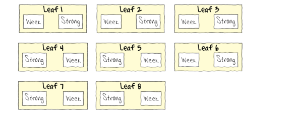
- Note that each level of the Treatment (Strong and Week) are applied to each Leaf (Block)
- Note that Treatments are randomly applied
- The Treatment effect is the mean difference between Treatment pairs per leaf
- Blocking in this way is very useful when spatial or temporal heterogeneity is likely to add noise that could make it difficualt to detect a difference between Treatments. Hence it is a way of experimentally reducing unexplained variation (compared to nesting which involves statistical reduction of unexplained variation).
Since each level of treatment was applied to each leaf, the data represents a randomized block design with leaves as blocks.
The variable LEAF contains a list of Leaf identification numbers and is supposed to represent a factorial blocking variable. However, because the contents of this variable are numbers, R initially treats them as numbers, and therefore considers the variable to be numeric rather than categorical. In order to force R to treat this variable as a factor (categorical) it is necessary to first convert this numeric variable into a factor (HINT).tobacco$LEAF <- as.factor(tobacco$LEAF)
- What are the main hypotheses being tested?
- H0 Factor A:
- H0 Factor B:
- H0 Factor A:
- In the table below, list the assumptions of a randomized block design along with how violations of each assumption are diagnosed and/or the risks of violations are minimized.
-
Assumption Diagnostic/Risk Minimization I. II. III. IV. - Is the proposed model
balanced?
(Yor N)
Show codereplications(NUMBER ~ LEAF + TREATMENT, data = tobacco)
LEAF TREATMENT 2 8!is.list(replications(NUMBER ~ LEAF + TREATMENT, data = tobacco))
[1] TRUE
-
- There are a number of
ways of diagnosing block by within block interactions.
- The simplest method is to plot the number of lesions for each treatment and leaf combination (ie. an
interaction plot
(HINT). Any evidence of an interaction? Note that we cannot formally test for an interaction because we don't have replicates for each treatment-leaf combination!
- We can also examine the residual plot from the fitted linear
model. A curvilinear pattern in which the residual values switch from positive to negative
and back again (or visa versa) over the range of predicted values implies that the scale
(magnitude but not polarity) of the main treatment effects differs substantially across the range
of blocks. (HINT). Any evidence of an interaction?
- Perform a Tukey's test for non-additivity evaluated at α = 0.10 or even &alpha = 0.25. This (curvilinear test)
formally tests for the presence of a quadratic trend in the relationship between residuals and
predicted values. As such, it too is only appropriate for simple interactions of scale.
(HINT). Any evidence of an interaction?
- Examine a lattice graphic to determine the consistency of the effect across each of the blocks(HINT).
Show codelibrary(car) interaction.plot(tobacco$LEAF, tobacco$TREATMENT, tobacco$NUMBER)
 Show ggplot code
library(ggplot2) ggplot(tobacco, aes(y = NUMBER, x = LEAF, group = TREATMENT, color = TREATMENT)) + geom_line()
 Show code
residualPlots(lm(NUMBER ~ LEAF + TREATMENT, data = tobacco))
Test stat Pr(>|t|) LEAF NA NA TREATMENT NA NA Tukey test -0.18 0.858
residualPlots(lm(NUMBER ~ LEAF + TREATMENT, data = tobacco))

Test stat Pr(>|t|) LEAF NA NA TREATMENT NA NA Tukey test -0.18 0.858
Show codelibrary(alr3)
Error in library(alr3): there is no package called 'alr3'
tukey.nonadd.test(lm(NUMBER ~ LEAF + TREATMENT, data = tobacco))
Error in eval(expr, envir, enclos): could not find function "tukey.nonadd.test"
Show codelibrary(ggplot2) ggplot(tobacco, aes(y = NUMBER, x = TREATMENT)) + geom_point() + facet_wrap(~LEAF)

# print(barchart(NUMBER~TREATMENT|LEAF, data=tobacco)) - The simplest method is to plot the number of lesions for each treatment and leaf combination (ie. an
interaction plot
(HINT). Any evidence of an interaction? Note that we cannot formally test for an interaction because we don't have replicates for each treatment-leaf combination!
- Analyse these data with a classic
randomized block ANOVA
(HINT) to test the H0 that there is no difference in the number of lesions produced by the different strength viruses. Complete the table below.
Show traditional code
tobacco.aov <- aov(NUMBER ~ TREATMENT + Error(LEAF), data = tobacco) summary(tobacco.aov)
Error: LEAF Df Sum Sq Mean Sq F value Pr(>F) Residuals 7 292.1 41.73 Error: Within Df Sum Sq Mean Sq F value Pr(>F) TREATMENT 1 248.3 248.34 17.17 0.00433 ** Residuals 7 101.2 14.46 --- Signif. codes: 0 '***' 0.001 '**' 0.01 '*' 0.05 '.' 0.1 ' ' 1Show lme codelibrary(nlme) # Fit random intercept model tobacco.lme <- lme(NUMBER ~ TREATMENT, random = ~1 | LEAF, data = tobacco, method = "REML") # Fit random intercept and slope model tobacco.lme1 <- lme(NUMBER ~ TREATMENT, random = ~TREATMENT | LEAF, data = tobacco, method = "REML") AIC(tobacco.lme, tobacco.lme1)
df AIC obacco.lme 4 96.70799 obacco.lme1 6 100.67049
anova(tobacco.lme, tobacco.lme1)
Model df AIC BIC logLik Test L.Ratio p-value obacco.lme 1 4 96.70799 99.26422 -44.35400 obacco.lme1 2 6 100.67049 104.50484 -44.33525 1 vs 2 0.03749921 0.9814
# Random intercepts and slope model does not fit the data better Use simpler random intercepts model summary(tobacco.lme)
Linear mixed-effects model fit by REML Data: tobacco AIC BIC logLik 96.70799 99.26422 -44.354 Random effects: Formula: ~1 | LEAF (Intercept) Residual StdDev: 3.69221 3.802924 Fixed effects: NUMBER ~ TREATMENT Value Std.Error DF t-value p-value (Intercept) 34.94013 1.873988 7 18.644800 0.0000 TREATMENTWeak -7.87938 1.901462 7 -4.143855 0.0043 Correlation: (Intr) TREATMENTWeak -0.507 Standardized Within-Group Residuals: Min Q1 Med Q3 Max -1.61850358 -0.48452374 0.01133376 0.40899999 1.42778213 Number of Observations: 16 Number of Groups: 8# Calculate the confidence interval for the effect size of the main effect of season intervals(tobacco.lme)
Approximate 95% confidence intervals Fixed effects: lower est. upper (Intercept) 30.50885 34.940130 39.371407 TREATMENTWeak -12.37562 -7.879381 -3.383139 attr(,"label") [1] "Fixed effects:" Random Effects: Level: LEAF lower est. upper sd((Intercept)) 1.580513 3.69221 8.625313 Within-group standard error: lower est. upper 2.252270 3.802924 6.421178# Examine the ANOVA table with Type I (sequential) SS anova(tobacco.lme)
numDF denDF F-value p-value (Intercept) 1 7 368.5003 <.0001 TREATMENT 1 7 17.1715 0.0043
library(broom) tidy(tobacco.lme, conf.int = TRUE)
group level term estimate 1 LEAF L1 (Intercept) 34.586218 2 LEAF L2 (Intercept) 33.399516 3 LEAF L3 (Intercept) 34.228954 4 LEAF L4 (Intercept) 32.379685 5 LEAF L5 (Intercept) 33.700202 6 LEAF L6 (Intercept) 38.442435 7 LEAF L7 (Intercept) 40.561728 8 LEAF L8 (Intercept) 32.222302 9 LEAF L1 TREATMENTWeak -7.879381 10 LEAF L2 TREATMENTWeak -7.879381 11 LEAF L3 TREATMENTWeak -7.879381 12 LEAF L4 TREATMENTWeak -7.879381 13 LEAF L5 TREATMENTWeak -7.879381 14 LEAF L6 TREATMENTWeak -7.879381 15 LEAF L7 TREATMENTWeak -7.879381 16 LEAF L8 TREATMENTWeak -7.879381
tidy(tobacco.lme, conf.int = TRUE, effects = "fixed")
# A tibble: 2 x 5 term estimate std.error statistic p.value <chr> <dbl> <dbl> <dbl> <dbl> 1 (Intercept) 34.9 1.87 18.6 0.000000317 2 TREATMENTWeak -7.88 1.90 -4.14 0.00433
glance(tobacco.lme)
# A tibble: 1 x 5 sigma logLik AIC BIC deviance <dbl> <dbl> <dbl> <dbl> <lgl> 1 3.80 -44.4 96.7 99.3 NA
Show lmer codelibrary(lme4) # Fit random intercepts model tobacco.lmer <- lmer(NUMBER ~ TREATMENT + (1 | LEAF), data = tobacco, REML = TRUE) # Fit random intercepts and slope model tobacco.lmer1 <- lmer(NUMBER ~ TREATMENT + (TREATMENT | LEAF), data = tobacco, REML = TRUE, control = lmerControl(check.nobs.vs.nRE = "ignore")) AIC(tobacco.lmer, tobacco.lmer1)
df AIC obacco.lmer 4 96.70799 obacco.lmer1 6 100.67049
anova(tobacco.lmer, tobacco.lmer1)
Data: tobacco Models: obacco.lmer: NUMBER ~ TREATMENT + (1 | LEAF) obacco.lmer1: NUMBER ~ TREATMENT + (TREATMENT | LEAF) Df AIC BIC logLik deviance Chisq Chi Df Pr(>Chisq) obacco.lmer 4 102.49 105.58 -47.246 94.491 obacco.lmer1 6 106.45 111.08 -47.224 94.448 0.0429 2 0.9788summary(tobacco.lmer)
Linear mixed model fit by REML ['lmerMod'] Formula: NUMBER ~ TREATMENT + (1 | LEAF) Data: tobacco REML criterion at convergence: 88.7 Scaled residuals: Min 1Q Median 3Q Max -1.61850 -0.48453 0.01133 0.40900 1.42778 Random effects: Groups Name Variance Std.Dev. LEAF (Intercept) 13.63 3.692 Residual 14.46 3.803 Number of obs: 16, groups: LEAF, 8 Fixed effects: Estimate Std. Error t value (Intercept) 34.940 1.874 18.645 TREATMENTWeak -7.879 1.901 -4.144 Correlation of Fixed Effects: (Intr) TREATMENTWk -0.507anova(tobacco.lmer)
Analysis of Variance Table Df Sum Sq Mean Sq F value TREATMENT 1 248.34 248.34 17.172# Calculate the confidence interval for the effect size of the main effect of season confint(tobacco.lmer)
2.5 % 97.5 % .sig01 0.000000 7.258832 .sigma 2.333872 6.361451 (Intercept) 31.216405 38.663855 TREATMENTWeak -11.147650 -3.931599
# Perform SAS-like p-value calculations (requires the lmerTest and pbkrtest package) library(lmerTest) tobacco.lmer <- lmer(NUMBER ~ TREATMENT + (1 | LEAF), data = tobacco) summary(tobacco.lmer)
Linear mixed model fit by REML t-tests use Satterthwaite approximations to degrees of freedom [ lmerMod] Formula: NUMBER ~ TREATMENT + (1 | LEAF) Data: tobacco REML criterion at convergence: 88.7 Scaled residuals: Min 1Q Median 3Q Max -1.61850 -0.48453 0.01133 0.40900 1.42778 Random effects: Groups Name Variance Std.Dev. LEAF (Intercept) 13.63 3.692 Residual 14.46 3.803 Number of obs: 16, groups: LEAF, 8 Fixed effects: Estimate Std. Error df t value Pr(>|t|) (Intercept) 34.940 1.874 11.332 18.645 7.38e-10 *** TREATMENTWeak -7.879 1.901 7.000 -4.144 0.00433 ** --- Signif. codes: 0 '***' 0.001 '**' 0.01 '*' 0.05 '.' 0.1 ' ' 1 Correlation of Fixed Effects: (Intr) TREATMENTWk -0.507anova(tobacco.lmer) # Satterthwaite denominator df method
Analysis of Variance Table of type III with Satterthwaite approximation for degrees of freedom Sum Sq Mean Sq NumDF DenDF F.value Pr(>F) TREATMENT 248.34 248.34 1 7 17.172 0.004328 ** --- Signif. codes: 0 '***' 0.001 '**' 0.01 '*' 0.05 '.' 0.1 ' ' 1anova(tobacco.lmer, ddf = "Kenward-Roger") # Kenward-Roger denominator df method
Analysis of Variance Table of type III with Kenward-Roger approximation for degrees of freedom Sum Sq Mean Sq NumDF DenDF F.value Pr(>F) TREATMENT 248.34 248.34 1 7 17.172 0.004328 ** --- Signif. codes: 0 '***' 0.001 '**' 0.01 '*' 0.05 '.' 0.1 ' ' 1# Examine the effect season via a likelihood ratio test tobacco.lmer1 <- lmer(NUMBER ~ TREATMENT + (1 | LEAF), data = tobacco, REML = F) tobacco.lmer2 <- lmer(NUMBER ~ TREATMENT + (TREATMENT | LEAF), data = tobacco, REML = F, control = lmerControl(check.nobs.vs.nRE = "ignore")) anova(tobacco.lmer1, tobacco.lmer2, test = "F")
Data: tobacco Models: object: NUMBER ~ TREATMENT + (1 | LEAF) ..1: NUMBER ~ TREATMENT + (TREATMENT | LEAF) Df AIC BIC logLik deviance Chisq Chi Df Pr(>Chisq) object 4 102.49 105.58 -47.246 94.491 ..1 6 106.45 111.08 -47.224 94.448 0.0429 2 0.9788library(broom) tidy(tobacco.lmer, conf.int = TRUE)
# A tibble: 4 x 7 term estimate std.error statistic conf.low conf.high group <chr> <dbl> <dbl> <dbl> <dbl> <dbl> <chr> 1 (Intercept) 34.9 1.87 18.6 31.3 38.6 fixed 2 TREATMENTWeak -7.88 1.90 -4.14 -11.6 -4.15 fixed 3 sd_(Intercept).LEAF 3.69 NA NA NA NA LEAF 4 sd_Observation.Residual 3.80 NA NA NA NA Residual
tidy(tobacco.lmer, conf.int = TRUE, effects = "fixed")
# A tibble: 2 x 6 term estimate std.error statistic conf.low conf.high <chr> <dbl> <dbl> <dbl> <dbl> <dbl> 1 (Intercept) 34.9 1.87 18.6 31.3 38.6 2 TREATMENTWeak -7.88 1.90 -4.14 -11.6 -4.15
glance(tobacco.lmer)
# A tibble: 1 x 6 sigma logLik AIC BIC deviance df.residual <dbl> <dbl> <dbl> <dbl> <dbl> <int> 1 3.80 -44.4 96.7 99.8 94.5 12
Show glmmTMB codelibrary(glmmTMB) # Fit random intercepts model tobacco.glmmTMB <- glmmTMB(NUMBER ~ TREATMENT + (1 | LEAF), data = tobacco) # Fit random intercepts and slope model tobacco.glmmTMB1 <- glmmTMB(NUMBER ~ TREATMENT + (TREATMENT | LEAF), data = tobacco) AIC(tobacco.glmmTMB, tobacco.glmmTMB1)
df AIC obacco.glmmTMB 4 102.4911 obacco.glmmTMB1 6 NA
anova(tobacco.glmmTMB, tobacco.glmmTMB1)
Data: tobacco Models: obacco.glmmTMB: NUMBER ~ TREATMENT + (1 | LEAF), zi=~0, disp=~1 obacco.glmmTMB1: NUMBER ~ TREATMENT + (TREATMENT | LEAF), zi=~0, disp=~1 Df AIC BIC logLik deviance Chisq Chi Df Pr(>Chisq) obacco.glmmTMB 4 102.49 105.58 -47.246 94.491 obacco.glmmTMB1 6 2summary(tobacco.glmmTMB)
Family: gaussian ( identity ) Formula: NUMBER ~ TREATMENT + (1 | LEAF) Data: tobacco AIC BIC logLik deviance df.resid 102.5 105.6 -47.2 94.5 12 Random effects: Conditional model: Groups Name Variance Std.Dev. LEAF (Intercept) 11.93 3.454 Residual 12.65 3.557 Number of obs: 16, groups: LEAF, 8 Dispersion estimate for gaussian family (sigma^2): 12.7 Conditional model: Estimate Std. Error z value Pr(>|z|) (Intercept) 34.940 1.753 19.93 < 2e-16 *** TREATMENTWeak -7.879 1.779 -4.43 9.42e-06 *** --- Signif. codes: 0 '***' 0.001 '**' 0.01 '*' 0.05 '.' 0.1 ' ' 1# Calculate the confidence interval for the effect size of the # main effect of season confint(tobacco.glmmTMB)
2.5 % 97.5 % Estimate cond.(Intercept) 31.504400 38.375863 34.940132 cond.TREATMENTWeak -11.365477 -4.393286 -7.879382 cond.Std.Dev.LEAF.(Intercept) 1.561741 7.637906 3.453756 sigma 2.179319 5.806593 3.557305
- Check the model diagnostics
- Residual plot
Show traditional codepar(mfrow = c(2, 2)) plot(lm(tobacco.aov))
 Show lme code
plot(tobacco.lme)

qqnorm(resid(tobacco.lme)) qqline(resid(tobacco.lme))

library(sjPlot) plot_grid(plot_model(tobacco.lme, type = "diag"))
 Show lmer code
plot(tobacco.lmer)

plot(fitted(tobacco.lmer), residuals(tobacco.lmer, type = "pearson", scaled = TRUE))

ggplot(fortify(tobacco.lmer), aes(y = .scresid, x = .fitted)) + geom_point()

qq.line = function(x) { # following four lines from base R's qqline() y <- quantile(x[!is.na(x)], c(0.25, 0.75)) x <- qnorm(c(0.25, 0.75)) slope <- diff(y)/diff(x) int <- y[1L] - slope * x[1L] return(c(int = int, slope = slope)) } QQline = qq.line(fortify(tobacco.lmer)$.scresid) ggplot(fortify(tobacco.lmer), aes(sample = .scresid)) + stat_qq() + geom_abline(intercept = QQline[1], slope = QQline[2])

qqnorm(resid(tobacco.lmer)) qqline(resid(tobacco.lmer))

library(sjPlot) plot_grid(plot_model(tobacco.lmer, type = "diag"))
 Show glmmTMB code
ggplot(data = NULL, aes(y = resid(tobacco.glmmTMB, type = "pearson"), x = fitted(tobacco.glmmTMB))) + geom_point()

QQline = qq.line(resid(tobacco.glmmTMB, type = "pearson")) ggplot(data = NULL, aes(sample = resid(tobacco.glmmTMB, type = "pearson"))) + stat_qq() + geom_abline(intercept = QQline[1], slope = QQline[2])

- Lets produce a quick partial (marginal) effects plot to represent
the model.
Show lme code
library(effects) plot(allEffects(tobacco.lme))

library(sjPlot) plot_model(tobacco.lme, type = "eff", terms = "TREATMENT")
 Show lmer code
library(effects) plot(allEffects(tobacco.lmer))

library(sjPlot) plot_model(tobacco.lmer, type = "eff", terms = "TREATMENT")
 Show glmmTMB code
library(ggeffects) # observation level effects averaged across margins p = ggaverage(tobacco.glmmTMB, terms = "TREATMENT") p = cbind(p, TREATMENT = levels(tobacco$TREATMENT)) ggplot(p, aes(y = predicted, x = TREATMENT)) + geom_pointrange(aes(ymin = conf.low, ymax = conf.high))

# marginal effects p = ggpredict(tobacco.glmmTMB, terms = "TREATMENT") p = cbind(p, TREATMENT = levels(tobacco$TREATMENT)) ggplot(p, aes(y = predicted, x = TREATMENT)) + geom_pointrange(aes(ymin = conf.low, ymax = conf.high))

- Where is the major variation in numbers of flatworms? Between (seasons, sites or stones)?
Show code for lme
library(nlme) nlme:::VarCorr(tobacco.lme)
LEAF = pdLogChol(1) Variance StdDev (Intercept) 13.63242 3.692210 Residual 14.46223 3.802924library(MuMIn) r.squaredGLMM(tobacco.lme)
R2m R2c 0.3707884 0.6761019
Show code for lmeVarCorr(tobacco.lmer)
Groups Name Std.Dev. LEAF (Intercept) 3.6922 Residual 3.8029
library(MuMIn) r.squaredGLMM(tobacco.lmer)
R2m R2c 0.3707882 0.6761026
source(system.file("misc/rsqglmm.R", package = "glmmTMB")) my_rsq(tobacco.lmer)
$family [1] "gaussian" $link [1] "identity" $Marginal [1] 0.3707882 $Conditional [1] 0.6761026
Show code for glmmTMBVarCorr(tobacco.glmmTMB)
Conditional model: Groups Name Std.Dev. LEAF (Intercept) 3.4538 Residual 3.5573
source(system.file("misc/rsqglmm.R", package = "glmmTMB")) my_rsq(tobacco.glmmTMB)
$family [1] "gaussian" $link [1] "identity" $Marginal [1] 0.4024406 $Conditional [1] 0.6923966
- Finally, construct an appropriate summary figure
to accompany the above analyses. Note that this should use the correct replicates for depicting error.
Show lme code
library(effects) tobacco.eff = as.data.frame(Effect("TREATMENT", tobacco.lme)) ggplot(tobacco.eff, aes(y = fit, x = TREATMENT)) + geom_pointrange(aes(ymin = lower, ymax = upper)) + scale_y_continuous("Mean number of lesions") + theme_classic()

# OR manually newdata <- data.frame(TREATMENT = levels(tobacco$TREATMENT)) Xmat <- model.matrix(~TREATMENT, data = newdata) coefs <- fixef(tobacco.lme) fit <- as.vector(coefs %*% t(Xmat)) se <- sqrt(diag(Xmat %*% vcov(tobacco.lme) %*% t(Xmat))) q = qt(0.975, df = nrow(tobacco.lme$data) - length(coefs) - 2) newdata <- cbind(newdata, fit = fit, lower = fit - 2 * se, upper = fit + 2 * se) ggplot(newdata, aes(y = fit, x = TREATMENT)) + geom_errorbar(aes(ymin = lower, ymax = upper), width = 0.05) + geom_point(size = 2) + scale_y_continuous("Mean number of lesions") + theme_classic() + theme(axis.title.x = element_blank(), axis.title.y = element_text(vjust = 2, size = rel(1.25)), panel.margin = unit(c(0.5, 0.5, 0.5, 2), "lines"))
 Show lmer code
library(effects) tobacco.eff = as.data.frame(Effect("TREATMENT", tobacco.lmer)) ggplot(tobacco.eff, aes(y = fit, x = TREATMENT)) + geom_pointrange(aes(ymin = lower, ymax = upper)) + scale_y_continuous("Mean number of lesions") + theme_classic()

# OR manually newdata <- data.frame(TREATMENT = levels(tobacco$TREATMENT)) Xmat <- model.matrix(~TREATMENT, data = newdata) coefs <- fixef(tobacco.lmer) fit <- as.vector(coefs %*% t(Xmat)) se <- sqrt(diag(Xmat %*% vcov(tobacco.lmer) %*% t(Xmat))) q = qt(0.975, df = df.residual(tobacco.lmer)) newdata <- cbind(newdata, fit = fit, lower = fit - 2 * se, upper = fit + 2 * se) ggplot(newdata, aes(y = fit, x = TREATMENT)) + geom_errorbar(aes(ymin = lower, ymax = upper), width = 0.05) + geom_point(size = 2) + scale_y_continuous("Mean number of lesions") + theme_classic() + theme(axis.title.x = element_blank(), axis.title.y = element_text(vjust = 2, size = rel(1.25)), panel.margin = unit(c(0.5, 0.5, 0.5, 2), "lines"))
 Show glmmTMB code
newdata <- data.frame(TREATMENT = levels(tobacco$TREATMENT)) Xmat <- model.matrix(~TREATMENT, data = newdata) coefs <- fixef(tobacco.glmmTMB)[[1]] fit <- as.vector(coefs %*% t(Xmat)) se <- sqrt(diag(Xmat %*% vcov(tobacco.glmmTMB)[[1]] %*% t(Xmat))) q = qt(0.975, df = df.residual(tobacco.glmmTMB)) newdata <- cbind(newdata, fit = fit, lower = fit - 2 * se, upper = fit + 2 * se) ggplot(newdata, aes(y = fit, x = TREATMENT)) + geom_errorbar(aes(ymin = lower, ymax = upper), width = 0.05) + geom_point(size = 2) + scale_y_continuous("Mean number of lesions") + theme_classic() + theme(axis.title.x = element_blank(), axis.title.y = element_text(vjust = 2, size = rel(1.25)), panel.margin = unit(c(0.5, 0.5, 0.5, 2), "lines"))

- Calculate approximate $R^2$
Show lme code
library(MuMIn) r.squaredGLMM(tobacco.lme)
R2m R2c 0.3707884 0.6761019
Show lmer codelibrary(MuMIn) r.squaredGLMM(tobacco.lmer)
R2m R2c 0.3707882 0.6761026
source(system.file("misc/rsqglmm.R", package = "glmmTMB")) my_rsq(tobacco.lmer)
$family [1] "gaussian" $link [1] "identity" $Marginal [1] 0.3707882 $Conditional [1] 0.6761026
Show glmmTMB codesource(system.file("misc/rsqglmm.R", package = "glmmTMB")) my_rsq(tobacco.glmmTMB)
$family [1] "gaussian" $link [1] "identity" $Marginal [1] 0.4024406 $Conditional [1] 0.6923966
Repeated measures
Freitas, Olsen, Knutsen, Albretsen, Moland, and Genner (2015)
investigated the effects of sea temperature on the habitat selection and habitat use of acoustically
tagged Atlantic code (Gadus morhua) along the coast of Norway. One aspect that was of particular
interest was the relationship between the depth that the cod were found at and the water temperature
(at the surface).
For each of the 48 tagged cod, the mean daytime and nighttime depth was calculated for each day the individual was tracked along with the average temperature of the water at the surface during the associated periods of time. Since each cod was repeatedly sampled, a mixed effects model (that accounts for correlations within individuals) is appropriate.
Download freitas data set| Format of freitas.csv data files | ||||||||||||||||||||||||||||||||||||
|---|---|---|---|---|---|---|---|---|---|---|---|---|---|---|---|---|---|---|---|---|---|---|---|---|---|---|---|---|---|---|---|---|---|---|---|---|
|
||||||||||||||||||||||||||||||||||||
|
 |
|||||||||||||||||||||||||||||||||||
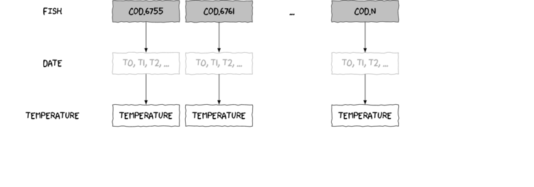
Note, some of the parameters estimated here differ slightly from those presented in
Freitas, Olsen, Knutsen, et al. (2015).
I suspect this is simply to do with rounding of the data. The overall conclusions are not affected..
Differences are also likely due to differences in sample size reported in Freitas, Olsen, Knutsen, et al. (2015)
and those present in the data they provide.
Open the freitas data file.
freitas <- read.csv("../downloads/data/freitas.csv", header = T, sep = ",", strip.white = T) head(freitas)
FISH Date DEPTH_MEAN_DAY DEPTH_MEAN_NIGHT TEMPERATURE_1M 1 Cod_6755 2013/06/28 19.64417 19.59565 18.00542 2 Cod_6755 2013/06/29 19.98276 19.72679 17.75596 3 Cod_6755 2013/06/30 19.94709 20.04062 17.18113 4 Cod_6755 2013/07/01 19.96828 19.94154 17.49952 5 Cod_6755 2013/07/02 17.74378 19.93000 17.60138 6 Cod_6755 2013/07/03 14.47237 19.12308 17.60550
In preparation we should make sure that FISH is declared as a categorical variable. It would also be a good idea to ensure that DATE is considered a Date object and that it is also represented by a numberic version (perhaps the number of days since the start of sampling) that can be used in models.
library(tidyverse) library(lubridate) freitas = freitas %>% mutate(FISH = factor(FISH), Date = as.Date(Date), Dt = as.integer(Date - min(Date)))
We will explore the relationship between daytime dive depth and surface temperature. Data were collected over up to 159 days. It is likely that water temperatures would drift over this time, and therefore there is potential for temporal autocorrelation. This should be addressed.
- Perform exploratory data analysis
Show code
## Explore the distribution of response (DEPTH_MEAN_DAY) within ## each FISH ggplot(freitas, aes(y = DEPTH_MEAN_DAY, x = FISH)) + geom_boxplot() + theme(axis.text.x = element_text(angle = 45, hjust = 1))

## Explore the distribution of covariate (TEMPERATURE_1M) within ## each FISH ggplot(freitas, aes(y = TEMPERATURE_1M, x = FISH)) + geom_boxplot() + theme(axis.text.x = element_text(angle = 45, hjust = 1))

## Explore the relationships between DEPTH_MEAN_DAY and ## TEMPERATURE_1M within each FISH and color the points according ## to Dt so as to explore temporal dependency. ggplot(freitas, aes(y = DEPTH_MEAN_DAY, x = TEMPERATURE_1M)) + geom_point(aes(color = Dt)) + facet_wrap(~FISH) + geom_smooth(method = "lm")

## Estimate the degree to which the depth/temperature relationship ## is likely to differ between individual fish. library(car) residualPlots(lm(DEPTH_MEAN_DAY ~ FISH * TEMPERATURE_1M, freitas))

Test stat Pr(>|t|) FISH NA NA TEMPERATURE_1M 2.301 0.021 Tukey test -7.040 0.000
- Fit a range of candidate models
- random intercept model with TEMPERATURE_1M fixed component
- random intercept/slope (TEMPERATURE_1M) model with TEMPERATURE_1M fixed component
Show lme code## Compare random intercept model to a random intercept/slope model. Use ## REML to do so. freitas.lme = lme(DEPTH_MEAN_DAY ~ TEMPERATURE_1M, random = ~1 | FISH, data = freitas, method = "REML", na.action = na.omit) freitas.lme1 = lme(DEPTH_MEAN_DAY ~ TEMPERATURE_1M, random = ~TEMPERATURE_1M | FISH, data = freitas, method = "REML", na.action = na.omit) anova(freitas.lme, freitas.lme1)
Model df AIC BIC logLik Test L.Ratio p-value freitas.lme 1 4 28655.09 28681.26 -14323.55 freitas.lme1 2 6 27132.29 27171.56 -13560.15 1 vs 2 1526.798 <.0001
# The newer nlmnb optimizer can be a bit flaky, try the BFGS optimizer # instead freitas.lme2 = update(freitas.lme1, random = ~TEMPERATURE_1M | FISH, method = "REML", control = lmeControl(opt = "optim"), na.action = na.omit) anova(freitas.lme1, freitas.lme2)
Model df AIC BIC logLik freitas.lme1 1 6 27132.29 27171.56 -13560.15 freitas.lme2 2 6 27132.29 27171.56 -13560.15
Show lmer code## Compare random intercept model to a random intercept/slope model. Use ## REML to do so. freitas.lmer = lmer(DEPTH_MEAN_DAY ~ TEMPERATURE_1M + (1 | FISH), data = freitas, REML = TRUE, na.action = na.omit) freitas.lmer1 = lmer(DEPTH_MEAN_DAY ~ TEMPERATURE_1M + (TEMPERATURE_1M | FISH), data = freitas, REML = TRUE, na.action = na.omit) anova(freitas.lmer, freitas.lmer1)
Data: freitas Models: object: DEPTH_MEAN_DAY ~ TEMPERATURE_1M + (1 | FISH) ..1: DEPTH_MEAN_DAY ~ TEMPERATURE_1M + (TEMPERATURE_1M | FISH) Df AIC BIC logLik deviance Chisq Chi Df Pr(>Chisq) object 4 28649 28675 -14321 28641 ..1 6 27131 27170 -13559 27119 1522.6 2 < 2.2e-16 *** --- Signif. codes: 0 '***' 0.001 '**' 0.01 '*' 0.05 '.' 0.1 ' ' 1Show glmmTMB codeIt would seem that the model incorporating the random intercept/slope (TEMPERATURE_1M) is 'best' so far.## Compare random intercept model to a random intercept/slope model. Use ## REML to do so. freitas.glmmTMB = glmmTMB(DEPTH_MEAN_DAY ~ TEMPERATURE_1M + (1 | FISH), data = freitas, na.action = na.omit) freitas.glmmTMB1 = glmmTMB(DEPTH_MEAN_DAY ~ TEMPERATURE_1M + (TEMPERATURE_1M | FISH), data = freitas, na.action = na.omit) anova(freitas.glmmTMB, freitas.glmmTMB1)
Data: freitas Models: freitas.glmmTMB: DEPTH_MEAN_DAY ~ TEMPERATURE_1M + (1 | FISH), zi=~0, disp=~1 freitas.glmmTMB1: DEPTH_MEAN_DAY ~ TEMPERATURE_1M + (TEMPERATURE_1M | FISH), zi=~0, disp=~1 Df AIC BIC logLik deviance Chisq Chi Df Pr(>Chisq) freitas.glmmTMB 4 28649 28675 -14321 28641 freitas.glmmTMB1 6 27131 27170 -13559 27119 1522.6 2 < 2.2e-16 *** --- Signif. codes: 0 '***' 0.001 '**' 0.01 '*' 0.05 '.' 0.1 ' ' 1 - Group mean centering - center the observations within each fish by subtracting the observed values from the mean of the fish
- Grand mean centering - center the fish group means within the entire data set by subtracting the group means from the grand mean
- Generate the group and grand mean centered variables
Show code
freitas.1 = freitas %>% group_by(FISH) %>% mutate(grp.mean = mean(TEMPERATURE_1M), Temp.grpmc = TEMPERATURE_1M - grp.mean) %>% ungroup freitas.2 = freitas %>% group_by(FISH) %>% summarize(grp.mean = mean(TEMPERATURE_1M)) %>% ungroup %>% mutate(Temp.grdmc = grp.mean - mean(grp.mean)) freitas.gc = freitas.1 %>% full_join(freitas.2)
- Refit the above candidate models
Show lme code
## Compare random intercept model to a random intercept/slope model. Use ## REML to do so. freitas.lme2 = lme(DEPTH_MEAN_DAY ~ Temp.grpmc + Temp.grdmc, random = ~1 | FISH, data = freitas.gc, method = "REML", na.action = na.omit) freitas.lme3 = lme(DEPTH_MEAN_DAY ~ Temp.grpmc + Temp.grdmc, random = ~Temp.grpmc | FISH, data = freitas.gc, method = "REML", na.action = na.omit) anova(freitas.lme2, freitas.lme3)
Model df AIC BIC logLik Test L.Ratio p-value freitas.lme2 1 5 28655.26 28687.98 -14322.63 freitas.lme3 2 7 27122.27 27168.07 -13554.13 1 vs 2 1536.991 <.0001
freitas.lme1a = update(freitas.lme1, data = freitas.gc, method = "ML", control = lmeControl(opt = "optim")) anova(freitas.lme1a, update(freitas.lme3, method = "ML"))
Model df AIC BIC logLik Test L.Ratio p-value freitas.lme1a 1 6 27130.62 27169.88 -13559.31 update(freitas.lme3, method = "ML") 2 7 27119.84 27165.65 -13552.92 1 vs 2 12.7798 4e-04
Show lmer code## Compare random intercept model to a random intercept/slope model. Use ## REML to do so. freitas.lmer2 = lmer(DEPTH_MEAN_DAY ~ Temp.grpmc + Temp.grdmc + (1 | FISH), data = freitas.gc, REML = TRUE, na.action = na.omit) freitas.lmer3 = lmer(DEPTH_MEAN_DAY ~ Temp.grpmc + Temp.grdmc + (Temp.grpmc | FISH), data = freitas.gc, REML = TRUE, na.action = na.omit) anova(freitas.lmer2, freitas.lmer3)
Data: freitas.gc Models: object: DEPTH_MEAN_DAY ~ Temp.grpmc + Temp.grdmc + (1 | FISH) ..1: DEPTH_MEAN_DAY ~ Temp.grpmc + Temp.grdmc + (Temp.grpmc | FISH) Df AIC BIC logLik deviance Chisq Chi Df Pr(>Chisq) object 5 28649 28682 -14320 28639 ..1 7 27120 27166 -13553 27106 1533.1 2 < 2.2e-16 *** --- Signif. codes: 0 '***' 0.001 '**' 0.01 '*' 0.05 '.' 0.1 ' ' 1freitas.lmer1 = update(freitas.lmer1, data = freitas.gc) anova(freitas.lmer1, freitas.lmer3)
Data: freitas.gc Models: freitas.lmer1: DEPTH_MEAN_DAY ~ TEMPERATURE_1M + (TEMPERATURE_1M | FISH) freitas.lmer3: DEPTH_MEAN_DAY ~ Temp.grpmc + Temp.grdmc + (Temp.grpmc | FISH) Df AIC BIC logLik deviance Chisq Chi Df Pr(>Chisq) freitas.lmer1 6 27131 27170 -13559 27119 freitas.lmer3 7 27120 27166 -13553 27106 12.78 1 0.0003504 *** --- Signif. codes: 0 '***' 0.001 '**' 0.01 '*' 0.05 '.' 0.1 ' ' 1Show glmmTMB codeIt would seem that the model incorporating the random intercept/slope (TEMPERATURE_1M) is 'best' so far.## Compare random intercept model to a random intercept/slope model. Use ## REML to do so. freitas.glmmTMB2 = glmmTMB(DEPTH_MEAN_DAY ~ Temp.grpmc + Temp.grdmc + (1 | FISH), data = freitas.gc, na.action = na.omit) freitas.glmmTMB3 = glmmTMB(DEPTH_MEAN_DAY ~ Temp.grpmc + Temp.grdmc + (Temp.grpmc | FISH), data = freitas.gc, na.action = na.omit) anova(freitas.glmmTMB2, freitas.glmmTMB3)
Data: freitas.gc Models: freitas.glmmTMB2: DEPTH_MEAN_DAY ~ Temp.grpmc + Temp.grdmc + (1 | FISH), zi=~0, disp=~1 freitas.glmmTMB3: DEPTH_MEAN_DAY ~ Temp.grpmc + Temp.grdmc + (Temp.grpmc | FISH), zi=~0, disp=~1 Df AIC BIC logLik deviance Chisq Chi Df Pr(>Chisq) freitas.glmmTMB2 5 28649 28682 -14320 28639 freitas.glmmTMB3 7 27120 27166 -13553 27106 1533.1 2 < 2.2e-16 *** --- Signif. codes: 0 '***' 0.001 '**' 0.01 '*' 0.05 '.' 0.1 ' ' 1freitas.glmmTMB1 = update(freitas.glmmTMB1, data = freitas.gc) anova(freitas.glmmTMB1, freitas.glmmTMB3)
Data: freitas.gc Models: freitas.glmmTMB1: DEPTH_MEAN_DAY ~ TEMPERATURE_1M + (TEMPERATURE_1M | FISH), zi=~0, disp=~1 freitas.glmmTMB3: DEPTH_MEAN_DAY ~ Temp.grpmc + Temp.grdmc + (Temp.grpmc | FISH), zi=~0, disp=~1 Df AIC BIC logLik deviance Chisq Chi Df Pr(>Chisq) freitas.glmmTMB1 6 27131 27170 -13559 27119 freitas.glmmTMB3 7 27120 27166 -13553 27106 12.78 1 0.0003504 *** --- Signif. codes: 0 '***' 0.001 '**' 0.01 '*' 0.05 '.' 0.1 ' ' 1 - Check the model diagnostics - validate the model
- Residual plots
Show lme codeplot(freitas.lme3)

qqnorm(resid(freitas.lme3)) qqline(resid(freitas.lme3))

freitas.mod.dat = freitas.lme3$data[-freitas.lme3$na.action, ] ggplot(data = NULL) + geom_point(aes(y = resid(freitas.lme3, type = "normalized"), x = freitas.mod.dat$Temp.grpmc))

ggplot(data = NULL) + geom_point(aes(y = resid(freitas.lme3, type = "normalized"), x = freitas.mod.dat$Temp.grdmc))

library(sjPlot) plot_grid(plot_model(freitas.lme3, type = "diag"))

## Explore temporal autocorrelation plot(ACF(freitas.lme3, resType = "normalized"), alpha = 0.05)
 Show lmer code
qq.line = function(x) { # following four lines from base R's qqline() y <- quantile(x[!is.na(x)], c(0.25, 0.75)) x <- qnorm(c(0.25, 0.75)) slope <- diff(y)/diff(x) int <- y[1L] - slope * x[1L] return(c(int = int, slope = slope)) } plot(freitas.lmer3)

QQline = qq.line(resid(freitas.lmer3, type = "pearson", scale = TRUE)) ggplot(data = NULL, aes(sample = resid(freitas.lmer3, type = "pearson", scale = TRUE))) + stat_qq() + geom_abline(intercept = QQline[1], slope = QQline[2])

qqnorm(resid(freitas.lmer3)) qqline(resid(freitas.lmer3))

ggplot(data = NULL, aes(y = resid(freitas.lmer3, type = "pearson", scale = TRUE), x = fitted(freitas.lmer3))) + geom_point()

ggplot(data = NULL, aes(y = resid(freitas.lmer3, type = "pearson", scale = TRUE), x = freitas.lmer3@frame$Temp.grpmc)) + geom_point()

ggplot(data = NULL, aes(y = resid(freitas.lmer3, type = "pearson", scale = TRUE), x = freitas.lmer3@frame$Temp.grdmc)) + geom_point()

library(sjPlot) plot_grid(plot_model(freitas.lmer3, type = "diag"))

## Explore temporal autocorrelation ACF.merMod <- function(object, maxLag, resType = c("pearson", "response", "deviance", "raw"), scaled = TRUE, re = names(object@flist[1]), ...) { resType <- match.arg(resType) res <- resid(object, type = resType, scaled = TRUE) res = split(res, object@flist[[re]]) if (missing(maxLag)) { maxLag <- min(c(maxL <- max(lengths(res)) - 1, as.integer(10 * log10(maxL + 1)))) } val <- lapply(res, function(el, maxLag) { N <- maxLag + 1L tt <- double(N) nn <- integer(N) N <- min(c(N, n <- length(el))) nn[1:N] <- n + 1L - 1:N for (i in 1:N) { tt[i] <- sum(el[1:(n - i + 1)] * el[i:n]) } array(c(tt, nn), c(length(tt), 2)) }, maxLag = maxLag) val0 <- rowSums(sapply(val, function(x) x[, 2])) val1 <- rowSums(sapply(val, function(x) x[, 1]))/val0 val2 <- val1/val1[1L] z <- data.frame(lag = 0:maxLag, ACF = val2) attr(z, "n.used") <- val0 class(z) <- c("ACF", "data.frame") z } plot(ACF(freitas.lmer3, resType = "pearson", scaled = TRUE), alpha = 0.05)
 Show glmmTMB codeWhilst the residual plots themselves appear reasonable (notwithstanding the lack of conformity in the qqnormal plots), there is definitely evidence of temporal autocorrelation.
qq.line = function(x) { # following four lines from base R's qqline() y <- quantile(x[!is.na(x)], c(0.25, 0.75)) x <- qnorm(c(0.25, 0.75)) slope <- diff(y)/diff(x) int <- y[1L] - slope * x[1L] return(c(int = int, slope = slope)) } ggplot(data = NULL, aes(y = resid(freitas.glmmTMB3, type = "pearson"), x = fitted(freitas.glmmTMB3))) + geom_point()

QQline = qq.line(resid(freitas.glmmTMB3, type = "pearson")) ggplot(data = NULL, aes(sample = resid(freitas.glmmTMB3, type = "pearson"))) + stat_qq() + geom_abline(intercept = QQline[1], slope = QQline[2])

ggplot(data = NULL, aes(y = resid(freitas.glmmTMB3, type = "pearson"), x = freitas.glmmTMB3$frame$Temp.grpmc)) + geom_point()

ggplot(data = NULL, aes(y = resid(freitas.glmmTMB3, type = "pearson"), x = freitas.glmmTMB3$frame$Temp.grdmc)) + geom_point()

library(sjPlot) plot_grid(plot_model(freitas.glmmTMB3, type = "diag"))
Error in UseMethod("rstudent"): no applicable method for 'rstudent' applied to an object of class "glmmTMB"## Explore temporal autocorrelation ACF.glmmTMB <- function(object, maxLag, resType = c("pearson", "response", "deviance", "raw"), re = names(object$modelInfo$reTrms$cond$flist[1]), ...) { resType <- match.arg(resType) res <- resid(object, type = resType) res = split(res, object$modelInfo$reTrms$cond$flist[[re]]) if (missing(maxLag)) { maxLag <- min(c(maxL <- max(lengths(res)) - 1, as.integer(10 * log10(maxL + 1)))) } val <- lapply(res, function(el, maxLag) { N <- maxLag + 1L tt <- double(N) nn <- integer(N) N <- min(c(N, n <- length(el))) nn[1:N] <- n + 1L - 1:N for (i in 1:N) { tt[i] <- sum(el[1:(n - i + 1)] * el[i:n]) } array(c(tt, nn), c(length(tt), 2)) }, maxLag = maxLag) val0 <- rowSums(sapply(val, function(x) x[, 2])) val1 <- rowSums(sapply(val, function(x) x[, 1]))/val0 val2 <- val1/val1[1L] z <- data.frame(lag = 0:maxLag, ACF = val2) attr(z, "n.used") <- val0 class(z) <- c("ACF", "data.frame") z } plot(ACF(freitas.glmmTMB3, resType = "pearson"), alpha = 0.05)

- Refit the random intercept/slope model accounting for temporal autocorrelation and re-perform model validation
Show lme code
## Fit with first order autocorrelation (AR1) freitas.lme4 = lme(DEPTH_MEAN_DAY ~ Temp.grpmc + Temp.grdmc, random = ~Temp.grpmc | FISH, data = freitas.gc, correlation = corAR1(form = ~Dt | FISH), method = "REML", na.action = na.omit) anova(freitas.lme3, freitas.lme4)
Model df AIC BIC logLik Test L.Ratio p-value freitas.lme3 1 7 27122.27 27168.07 -13554.13 freitas.lme4 2 8 22652.97 22705.32 -11318.49 1 vs 2 4471.296 <.0001
plot(freitas.lme4)

qqnorm(resid(freitas.lme4)) qqline(resid(freitas.lme4))

freitas.mod.dat = freitas.lme4$data[-freitas.lme4$na.action, ] ggplot(data = NULL) + geom_point(aes(y = resid(freitas.lme4, type = "normalized"), x = freitas.mod.dat$Temp.grpmc))

ggplot(data = NULL) + geom_point(aes(y = resid(freitas.lme4, type = "normalized"), x = freitas.mod.dat$Temp.grdmc))

library(sjPlot) plot_grid(plot_model(freitas.lme4, type = "diag"))

## Explore temporal autocorrelation plot(ACF(freitas.lme4, resType = "normalized"), alpha = 0.05)
 Show lmer code
## Fit with first order autocorrelation (AR1) freitas.gc1 = augment(freitas.lmer3) %>% group_by(FISH) %>% mutate(Resid = lag(.resid), Resid = ifelse(is.na(Resid), 0, Resid)) %>% ungroup freitas.lmer4 = lmer(DEPTH_MEAN_DAY ~ Temp.grpmc + Temp.grdmc + Resid + (Temp.grpmc | FISH), data = freitas.gc1, REML = TRUE, na.action = na.omit) freitas.lmer3a = lmer(DEPTH_MEAN_DAY ~ Temp.grpmc + Temp.grdmc + (Temp.grpmc | FISH), data = freitas.gc1, REML = TRUE, na.action = na.omit) anova(freitas.lmer3a, freitas.lmer4)
Error in anova.merMod(object = object, ... = ...): models were not all fitted to the same size of dataset
plot(freitas.lmer4)

QQline = qq.line(resid(freitas.lmer4, type = "pearson", scale = TRUE)) ggplot(data = NULL, aes(sample = resid(freitas.lmer4, type = "pearson", scale = TRUE))) + stat_qq() + geom_abline(intercept = QQline[1], slope = QQline[2])

qqnorm(resid(freitas.lmer4)) qqline(resid(freitas.lmer4))

ggplot(data = NULL, aes(y = resid(freitas.lmer4, type = "pearson", scale = TRUE), x = fitted(freitas.lmer4))) + geom_point()

ggplot(data = NULL, aes(y = resid(freitas.lmer4, type = "pearson", scale = TRUE), x = freitas.lmer4@frame$Temp.grpmc)) + geom_point()

ggplot(data = NULL, aes(y = resid(freitas.lmer4, type = "pearson", scale = TRUE), x = freitas.lmer4@frame$Temp.grdmc)) + geom_point()

plot_grid(plot_model(freitas.lmer4, type = "diag"))

plot(ACF(freitas.lmer4, resType = "pearson", scaled = TRUE), alpha = 0.05)
 Show glmmTMB codeIt is clear that accounting for temporal autocorrelation is an improvement.
## Fit with first order autocorrelation (AR1) freitas.glmmTMB4 = glmmTMB(DEPTH_MEAN_DAY ~ Temp.grpmc + Temp.grdmc + (Temp.grpmc | FISH) + ar1(as.factor(Dt) - 1 | FISH), data = freitas.gc) anova(freitas.glmmTMB3, freitas.glmmTMB4)
Data: freitas.gc Models: freitas.glmmTMB3: DEPTH_MEAN_DAY ~ Temp.grpmc + Temp.grdmc + (Temp.grpmc | FISH), zi=~0, disp=~1 freitas.glmmTMB4: DEPTH_MEAN_DAY ~ Temp.grpmc + Temp.grdmc + (Temp.grpmc | FISH) + , zi=~0, disp=~1 freitas.glmmTMB4: ar1(as.factor(Dt) - 1 | FISH), zi=~0, disp=~1 Df AIC BIC logLik deviance Chisq Chi Df Pr(>Chisq) freitas.glmmTMB3 7 27120 27166 -13553 27106 freitas.glmmTMB4 9 22330 22389 -11156 22312 4794 2 < 2.2e-16 *** --- Signif. codes: 0 '***' 0.001 '**' 0.01 '*' 0.05 '.' 0.1 ' ' 1ggplot(data = NULL, aes(y = resid(freitas.glmmTMB4, type = "pearson"), x = fitted(freitas.glmmTMB4))) + geom_point()
Error in if (REML) randomArg <- c(randomArg, "beta"): argument is of length zero
QQline = qq.line(resid(freitas.glmmTMB4, type = "pearson"))
Error in if (REML) randomArg <- c(randomArg, "beta"): argument is of length zero
ggplot(data = NULL, aes(sample = resid(freitas.glmmTMB4, type = "pearson"))) + stat_qq() + geom_abline(intercept = QQline[1], slope = QQline[2])
Error in if (REML) randomArg <- c(randomArg, "beta"): argument is of length zero
ggplot(data = NULL, aes(y = resid(freitas.glmmTMB4, type = "pearson"), x = freitas.glmmTMB4$frame$Temp.grpmc)) + geom_point()
Error in if (REML) randomArg <- c(randomArg, "beta"): argument is of length zero
ggplot(data = NULL, aes(y = resid(freitas.glmmTMB4, type = "pearson"), x = freitas.glmmTMB4$frame$Temp.grdmc)) + geom_point()
Error in if (REML) randomArg <- c(randomArg, "beta"): argument is of length zero

plot_grid(plot_model(freitas.glmmTMB3, type = "diag"))
Error in UseMethod("rstudent"): no applicable method for 'rstudent' applied to an object of class "glmmTMB"plot(ACF(freitas.glmmTMB4, resType = "pearson"), alpha = 0.05)
Error in if (REML) randomArg <- c(randomArg, "beta"): argument is of length zero
- Generate partial effects plots to assist with parameter interpretation
Show lme code
library(effects) plot(allEffects(freitas.lme4, residuals = TRUE))

library(sjPlot) ## The following uses Effect (from effects package) and therefore does ## not account for the offset library(gridExtra) grid.arrange(plot_model(freitas.lme4, type = "eff", terms = c("Temp.grpmc")), plot_model(freitas.lme4, type = "eff", terms = c("Temp.grdmc")))

# don't add show.data=TRUE - this will add raw data not partial # residuals library(ggeffects) # Not accounting for offset grid.arrange(plot(ggeffect(freitas.lmer4, terms = c("Temp.grpmc"))), plot(ggeffect(freitas.lmer4, terms = c("Temp.grdmc"))))

# Ignoring uncertainty in random effects plot(ggpredict(freitas.lme4, terms = c("Temp.grpmc")))
 Show lmer code
library(effects) plot(allEffects(freitas.lmer4, residuals = FALSE))

library(sjPlot) library(gridExtra) grid.arrange(plot_model(freitas.lmer4, type = "eff", terms = c("Temp.grpmc")), plot_model(freitas.lmer4, type = "eff", terms = c("Temp.grdmc")))

# don't add show.data=TRUE - this will add raw data not partial # residuals library(ggeffects) grid.arrange(plot(ggeffect(freitas.lmer4, terms = c("Temp.grpmc"))), plot(ggeffect(freitas.lmer4, terms = c("Temp.grdmc"))))
 Show glmmTMB code
library(ggeffects) # observation level effects averaged across margins p1 = ggaverage(freitas.glmmTMB4, terms = c("Temp.grpmc"))
Error in if (REML) randomArg <- c(randomArg, "beta"): argument is of length zero
g1 = ggplot(p1, aes(y = predicted, x = x, color = group, fill = group)) + geom_line()
Error in ggplot(p1, aes(y = predicted, x = x, color = group, fill = group)): object 'p1' not found
p2 = ggaverage(freitas.glmmTMB4, terms = c("Temp.grdmc"))
Error in if (REML) randomArg <- c(randomArg, "beta"): argument is of length zero
g2 = ggplot(p2, aes(y = predicted, x = x, color = group, fill = group)) + geom_line()
Error in ggplot(p2, aes(y = predicted, x = x, color = group, fill = group)): object 'p2' not found
grid.arrange(g1, g2)
Error in arrangeGrob(...): object 'g1' not found
p1 = ggpredict(freitas.glmmTMB4, terms = c("Temp.grpmc"))
Error in if (REML) randomArg <- c(randomArg, "beta"): argument is of length zero
g1 = ggplot(p1, aes(y = predicted, x = x, color = group, fill = group)) + geom_ribbon(aes(ymin = conf.low, ymax = conf.high), alpha = 0.3)
Error in ggplot(p1, aes(y = predicted, x = x, color = group, fill = group)): object 'p1' not found
p2 = ggpredict(freitas.glmmTMB4, terms = c("Temp.grdmc"))
Error in if (REML) randomArg <- c(randomArg, "beta"): argument is of length zero
g2 = ggplot(p2, aes(y = predicted, x = x, color = group, fill = group)) + geom_ribbon(aes(ymin = conf.low, ymax = conf.high), alpha = 0.3)
Error in ggplot(p2, aes(y = predicted, x = x, color = group, fill = group)): object 'p2' not found
grid.arrange(g1, g2)
Error in arrangeGrob(...): object 'g1' not found
- Explore the parameter estimates for the 'best' model
Show lme codeNote, these estimates differ from those presented by
Freitas, Olsen, Knutsen, et al. (2015)since the current model partitions the temperature effect into within and between FISH.summary(freitas.lme4)
Linear mixed-effects model fit by REML Data: freitas.gc AIC BIC logLik 22652.97 22705.32 -11318.49 Random effects: Formula: ~Temp.grpmc | FISH Structure: General positive-definite, Log-Cholesky parametrization StdDev Corr (Intercept) 3.0177495 (Intr) Temp.grpmc 0.3420687 -0.493 Residual 3.9576449 Correlation Structure: ARMA(1,0) Formula: ~Dt | FISH Parameter estimate(s): Phi1 0.840578 Fixed effects: DEPTH_MEAN_DAY ~ Temp.grpmc + Temp.grdmc Value Std.Error DF t-value p-value (Intercept) 18.396212 0.4758372 5087 38.66073 0 Temp.grpmc 0.731720 0.0724198 5087 10.10387 0 Temp.grdmc 1.389287 0.2846965 46 4.87989 0 Correlation: (Intr) Tmp.grp Temp.grpmc -0.303 Temp.grdmc 0.047 0.131 Standardized Within-Group Residuals: Min Q1 Med Q3 Max -3.7272001 -0.4424342 0.1051616 0.5542488 4.7100921 Number of Observations: 5136 Number of Groups: 48intervals(freitas.lme4)
Approximate 95% confidence intervals Fixed effects: lower est. upper (Intercept) 17.4633661 18.3962118 19.3290575 Temp.grpmc 0.5897461 0.7317201 0.8736941 Temp.grdmc 0.8162225 1.3892868 1.9623510 attr(,"label") [1] "Fixed effects:" Random Effects: Level: FISH lower est. upper sd((Intercept)) 2.3535795 3.0177495 3.86934558 sd(Temp.grpmc) 0.2073540 0.3420687 0.56430545 cor((Intercept),Temp.grpmc) -0.7880694 -0.4927940 -0.01317038 Correlation structure: lower est. upper Phi1 0.8137141 0.840578 0.8638587 attr(,"label") [1] "Correlation structure:" Within-group standard error: lower est. upper 3.667975 3.957645 4.270191library(broom) tidy(freitas.lme4, effects = "fixed")
# A tibble: 3 x 5 term estimate std.error statistic p.value <chr> <dbl> <dbl> <dbl> <dbl> 1 (Intercept) 18.4 0.476 38.7 6.62e-287 2 Temp.grpmc 0.732 0.0724 10.1 8.89e- 24 3 Temp.grdmc 1.39 0.285 4.88 1.31e- 5
glance(freitas.lme4)
# A tibble: 1 x 5 sigma logLik AIC BIC deviance <dbl> <dbl> <dbl> <dbl> <lgl> 1 3.96 -11318. 22653. 22705. NA
anova(freitas.lme4, type = "marginal")
numDF denDF F-value p-value (Intercept) 1 5087 1494.6520 <.0001 Temp.grpmc 1 5087 102.0881 <.0001 Temp.grdmc 1 46 23.8133 <.0001
Show lmer codesummary(freitas.lmer4)
Linear mixed model fit by REML t-tests use Satterthwaite approximations to degrees of freedom [ lmerMod] Formula: DEPTH_MEAN_DAY ~ Temp.grpmc + Temp.grdmc + Resid + (Temp.grpmc | FISH) Data: freitas.gc1 REML criterion at convergence: 23246 Scaled residuals: Min 1Q Median 3Q Max -7.5004 -0.4006 0.0400 0.4529 6.2210 Random effects: Groups Name Variance Std.Dev. Corr FISH (Intercept) 12.2138 3.495 Temp.grpmc 0.6256 0.791 -0.24 Residual 4.9468 2.224 Number of obs: 5135, groups: FISH, 48 Fixed effects: Estimate Std. Error df t value Pr(>|t|) (Intercept) 1.843e+01 5.059e-01 4.580e+01 36.433 < 2e-16 *** Temp.grpmc 1.055e+00 1.179e-01 4.619e+01 8.947 1.19e-11 *** Temp.grdmc 1.528e+00 3.083e-01 4.527e+01 4.956 1.05e-05 *** Resid 7.328e-01 9.619e-03 5.042e+03 76.176 < 2e-16 *** --- Signif. codes: 0 '***' 0.001 '**' 0.01 '*' 0.05 '.' 0.1 ' ' 1 Correlation of Fixed Effects: (Intr) Tmp.grp Tmp.grd Temp.grpmc -0.229 Temp.grdmc 0.002 0.011 Resid -0.001 0.000 0.000confint(freitas.lmer4)
2.5 % 97.5 % .sig01 2.8310360 4.24729685 .sig02 -0.4996978 0.06171169 .sig03 0.6418908 0.97829560 .sigma 2.1812124 2.26805877 (Intercept) 17.4409774 19.42292558 Temp.grpmc 0.8206815 1.28742912 Temp.grdmc 0.9236890 2.13217051 Resid 0.7139088 0.75162017
library(broom) tidy(freitas.lmer4, effects = "fixed", conf.int = TRUE)
term estimate std.error statistic conf.low conf.high 1 (Intercept) 18.4317060 0.50590159 36.433382 17.4401571 19.4232549 2 Temp.grpmc 1.0545608 0.11786699 8.947041 0.8235457 1.2855758 3 Temp.grdmc 1.5278004 0.30827400 4.955982 0.9235945 2.1320063 4 Resid 0.7327548 0.00961927 76.175716 0.7139014 0.7516082
glance(freitas.lmer4)
sigma logLik AIC BIC deviance df.residual 1 2.224148 -11622.98 23261.97 23314.32 23245.97 5127
anova(freitas.lmer4, type = "marginal")
Analysis of Variance Table Df Sum Sq Mean Sq F value Temp.grpmc 1 388.7 388.7 78.575 Temp.grdmc 1 121.7 121.7 24.605 Resid 1 28705.2 28705.2 5802.740## If you cant live without p-values... library(lmerTest) freitas.lmer4 <- update(freitas.lmer4) summary(freitas.lmer4)
Linear mixed model fit by REML ['lmerMod'] Formula: DEPTH_MEAN_DAY ~ Temp.grpmc + Temp.grdmc + Resid + (Temp.grpmc | FISH) Data: freitas.gc1 REML criterion at convergence: 23246 Scaled residuals: Min 1Q Median 3Q Max -7.5004 -0.4006 0.0400 0.4529 6.2210 Random effects: Groups Name Variance Std.Dev. Corr FISH (Intercept) 12.2138 3.495 Temp.grpmc 0.6256 0.791 -0.24 Residual 4.9468 2.224 Number of obs: 5135, groups: FISH, 48 Fixed effects: Estimate Std. Error t value (Intercept) 18.431706 0.505902 36.433 Temp.grpmc 1.054561 0.117867 8.947 Temp.grdmc 1.527800 0.308274 4.956 Resid 0.732755 0.009619 76.176 Correlation of Fixed Effects: (Intr) Tmp.grp Tmp.grd Temp.grpmc -0.229 Temp.grdmc 0.002 0.011 Resid -0.001 0.000 0.000anova(freitas.lmer4) # Satterthwaite denominator df method
Analysis of Variance Table Df Sum Sq Mean Sq F value Temp.grpmc 1 388.7 388.7 78.575 Temp.grdmc 1 121.7 121.7 24.605 Resid 1 28705.2 28705.2 5802.740anova(freitas.lmer4, ddf = "Kenward-Roger")
Analysis of Variance Table Df Sum Sq Mean Sq F value Temp.grpmc 1 388.7 388.7 78.575 Temp.grdmc 1 121.7 121.7 24.605 Resid 1 28705.2 28705.2 5802.740Error in detach("package:lmerTest"): invalid 'name' argumentShow glmmTMB codeConclusions:summary(freitas.glmmTMB4)
Family: gaussian ( identity ) Formula: DEPTH_MEAN_DAY ~ Temp.grpmc + Temp.grdmc + (Temp.grpmc | FISH) + ar1(as.factor(Dt) - 1 | FISH) Data: freitas.gc AIC BIC logLik deviance df.resid 22329.9 22388.8 -11155.9 22311.9 5127 Random effects: Conditional model: Groups Name Variance Std.Dev. Corr FISH (Intercept) 1.64382 1.2821 Temp.grpmc 0.01045 0.1022 -1.00 FISH.1 as.factor(Dt)0 26.23607 5.1221 0.96 (ar1) 0.96 (ar1) Residual 1.55672 1.2477 Number of obs: 5136, groups: FISH, 48 Dispersion estimate for gaussian family (sigma^2): 1.56 Conditional model: Estimate Std. Error z value Pr(>|z|) (Intercept) 18.20491 0.47251 38.53 < 2e-16 *** Temp.grpmc 0.42414 0.06639 6.39 1.68e-10 *** Temp.grdmc 1.25167 0.29124 4.30 1.73e-05 *** --- Signif. codes: 0 '***' 0.001 '**' 0.01 '*' 0.05 '.' 0.1 ' ' 1confint(freitas.glmmTMB4)
Error in is.nan(x): default method not implemented for type 'list'
- there is a positive effect of surface temperature on fish dive depth. Fish dive deeper as the surface temperature rises
- fish that occupy warmer temperatures dive deeper. Note, that this could be an artifact of the unbalanced sampling design. Some fish only have data from early on in the study when surface temperatures were warmer. Presumably, the researchers lost contact with some fish.
- Calculate $R^2$
Show lme code
library(MuMIn) r.squaredGLMM(freitas.lme4)
R2m R2c 0.2722327 0.5602155
Show lmer codelibrary(MuMIn) r.squaredGLMM(freitas.lmer4)
R2m R2c 0.4866274 0.8915978
Show glmmTMB codesource(system.file("misc/rsqglmm.R", package = "glmmTMB")) my_rsq(freitas.glmmTMB4)
$family [1] "gaussian" $link [1] "identity" $Marginal [1] 0.6159788 $Conditional [1] 0.8187547
- Generate an appropriate summary figure
Show lme code
## using the effects package note, there really is not a simple way ## to get the partial residuals out. There is a posible solution ## at ## https://stackoverflow.com/questions/43950459/use-ggplot-to-plot-partial-effects-obtained-with-effects-library ## However, 1) the residuals and thus partial residuals do not ## account for the random effect and 2) this cannot be done ## separately within multiple levels of a covariate This is why ## partial residuals are not drawn when multiline=TRUE is used in ## plot. library(tidyverse) library(effects) x = with(freitas.gc, seq(min(Temp.grpmc), max(Temp.grpmc), len = 100)) newdata = as.data.frame(Effect(c("Temp.grpmc"), freitas.lme4, xlevels = list(Temp.grpmc = x))) ## Create a new Temperature variable that is back on the original ## surface temperature scale newdata = newdata %>% mutate(TEMPERATURE_1M = Temp.grpmc + mean(freitas.gc$grp.mean)) ggplot(newdata, aes(y = fit, x = TEMPERATURE_1M)) + geom_ribbon(aes(ymin = lower, ymax = upper), alpha = 0.2) + geom_line() + scale_x_continuous(expression(Surface ~ temperature ~ (degree * C))) + scale_y_continuous("Mean dive depth (m)") + theme_classic()

## Of course, it can be done manually library(tidyverse) newdata = with(freitas.gc, expand.grid(Temp.grpmc = seq(min(Temp.grpmc), max(Temp.grpmc), len = 100), Temp.grdmc = 0)) Xmat = model.matrix(~Temp.grpmc + Temp.grdmc, data = newdata) coefs = fixef(freitas.lme4) fit = as.vector(coefs %*% t(Xmat)) se = sqrt(diag(Xmat %*% vcov(freitas.lme4) %*% t(Xmat))) q = qt(0.975, df = nrow(freitas.lme4$data) - length(coefs) - nrow(as.matrix(VarCorr(freitas.lme4)))) newdata = cbind(newdata, fit = fit, lower = fit - q * se, upper = fit + q * se) newdata = newdata %>% mutate(TEMPERATURE_1M = Temp.grpmc + mean(freitas.gc$grp.mean)) # now for the residuals resid = freitas.lme4$data Xmat = model.matrix(~Temp.grpmc + Temp.grdmc, data = resid) coefs = fixef(freitas.lme4) fit = as.vector(coefs %*% t(Xmat)) res = freitas.gc$DEPTH_MEAN_DAY - fit #doesnt account for random effects resid = cbind(resid, res = res, partial = fit + res) resid = resid %>% mutate(TEMPERATURE_1M = Temp.grpmc + mean(freitas.gc$grp.mean)) ggplot(newdata, aes(y = fit, x = TEMPERATURE_1M)) + geom_point(data = resid, aes(y = partial), size = 2, alpha = 0.1) + geom_ribbon(aes(ymin = lower, ymax = upper), alpha = 0.2) + geom_line() + scale_y_continuous("Mean diving depth (m)") + scale_x_continuous(expression(Surface ~ temperature ~ (degree * C))) + theme_classic() + theme(legend.position = c(0.5, 1), legend.justification = c(0.5, 1))
 Show lmer code
## using the effects package note, there really is not a simple way ## to get the partial residuals out. There is a posible solution ## at ## https://stackoverflow.com/questions/43950459/use-ggplot-to-plot-partial-effects-obtained-with-effects-library ## However, 1) the residuals and thus partial residuals do not ## account for the random effect and 2) this cannot be done ## separately within multiple levels of a covariate This is why ## partial residuals are not drawn when multiline=TRUE is used in ## plot. library(tidyverse) library(effects) x = with(freitas.gc, seq(min(Temp.grpmc), max(Temp.grpmc), len = 100)) newdata = as.data.frame(Effect(c("Temp.grpmc"), freitas.lmer4, xlevels = list(Temp.grpmc = x))) ## Create a new Temperature variable that is back on the original ## surface temperature scale newdata = newdata %>% mutate(TEMPERATURE_1M = Temp.grpmc + mean(freitas.gc$grp.mean)) ggplot(newdata, aes(y = fit, x = TEMPERATURE_1M)) + geom_ribbon(aes(ymin = lower, ymax = upper), alpha = 0.2) + geom_line() + scale_x_continuous(expression(Surface ~ temperature ~ (degree * C))) + scale_y_continuous("Mean dive depth (m)") + theme_classic()

## Of course, it can be done manually library(tidyverse) newdata = with(freitas.gc, expand.grid(Temp.grpmc = seq(min(Temp.grpmc), max(Temp.grpmc), len = 100), Temp.grdmc = 0, Resid = 0)) Xmat = model.matrix(~Temp.grpmc + Temp.grdmc + Resid, data = newdata) coefs = fixef(freitas.lmer4) fit = as.vector(coefs %*% t(Xmat)) se = sqrt(diag(Xmat %*% vcov(freitas.lmer4) %*% t(Xmat))) q = qt(0.975, df = df.residual(freitas.lmer4)) newdata = cbind(newdata, fit = fit, lower = fit - q * se, upper = fit + q * se) newdata = newdata %>% mutate(TEMPERATURE_1M = Temp.grpmc + mean(freitas.gc$grp.mean)) # now for the residuals resid = freitas.lmer4@frame Xmat = model.matrix(~Temp.grpmc + Temp.grdmc + Resid, data = resid) coefs = fixef(freitas.lmer4) fit = as.vector(coefs %*% t(Xmat)) res = freitas.lmer4@frame$DEPTH_MEAN_DAY - fit #doesnt account for random effects resid = cbind(resid, res = res, partial = fit + res) resid = resid %>% mutate(TEMPERATURE_1M = Temp.grpmc + mean(freitas.gc$grp.mean)) ggplot(newdata, aes(y = fit, x = TEMPERATURE_1M)) + geom_point(data = resid, aes(y = partial), size = 2, alpha = 0.1) + geom_ribbon(aes(ymin = lower, ymax = upper), alpha = 0.2) + geom_line() + scale_y_continuous("Mean diving depth (m)") + scale_x_continuous(expression(Surface ~ temperature ~ (degree * C))) + theme_classic() + theme(legend.position = c(0.5, 1), legend.justification = c(0.5, 1))
 Show glmmTMB code
## Of course, it can be done manually library(tidyverse) newdata = with(freitas.gc, expand.grid(Temp.grpmc = seq(min(Temp.grpmc), max(Temp.grpmc), len = 100), Temp.grdmc = 0, Resid = 0)) Xmat = model.matrix(~Temp.grpmc + Temp.grdmc, data = newdata) coefs = fixef(freitas.glmmTMB4)[[1]] fit = as.vector(coefs %*% t(Xmat)) se = sqrt(diag(Xmat %*% vcov(freitas.glmmTMB4)[[1]] %*% t(Xmat))) q = qt(0.975, df = df.residual(freitas.glmmTMB4)) newdata = cbind(newdata, fit = fit, lower = fit - q * se, upper = fit + q * se) newdata = newdata %>% mutate(TEMPERATURE_1M = Temp.grpmc + mean(freitas.gc$grp.mean)) # now for the residuals resid = freitas.glmmTMB4$frame Xmat = model.matrix(~Temp.grpmc + Temp.grdmc, data = resid) coefs = fixef(freitas.glmmTMB4)[[1]] fit = as.vector(coefs %*% t(Xmat)) res = freitas.glmmTMB4$frame$DEPTH_MEAN_DAY - fit #doesnt account for random effects resid = cbind(resid, res = res, partial = fit + res) resid = resid %>% mutate(TEMPERATURE_1M = Temp.grpmc + mean(freitas.gc$grp.mean)) ggplot(newdata, aes(y = fit, x = TEMPERATURE_1M)) + geom_point(data = resid, aes(y = partial), size = 2, alpha = 0.1) + geom_ribbon(aes(ymin = lower, ymax = upper), alpha = 0.2) + geom_line() + scale_y_continuous("Mean diving depth (m)") + scale_x_continuous(expression(Surface ~ temperature ~ (degree * C))) + theme_classic() + theme(legend.position = c(0.5, 1), legend.justification = c(0.5, 1))

The above model will explore the relationship between temperature and dive depth. However, the temperature
various both within a fish and between fish. We may wish to tease them appart.
Freitas, Olsen, Knutsen, et al. (2015) did not do this as it was
likely not of interest to them, however, for the sake of demonstration, we will do it here.
To partition the covariate effects into the two levels of the hierarchy (between and within FISH) within the model, we need to create two new representations of the temperature variable:
Two factor Randomized Block ANOVA
To investigate differential metabolic plasticity in barramundi (Lates calcarifer),
Norin, Malte, Clark, and Konarzewski (2016)
exposed juvenile barramundi to various environmental changes (increased temperature,
decreased salinity and increased hypoxia) as well as control conditions.
Metabolic plasticity was calculated as the percentage difference in standard metabolic rate between
the various treatment conditions and the standard metabolic rate under control conditions.
They were interested in whether there was a relationship between metabolic plasticity and typical (control) metabolism and
how the different treatment conditions impact on this relationship.
A total of 60 barramundi juveniles were subject to each of the three conditions (high temperature, low salinity and hypoxia) in addition to control conditions. Fish mass was also recorded as a covariate as this is known to influence metabolic parameters.
Download Starling data set| Format of norin.csv data files | |||||||||||||||||||||||||||||||||||||||||||||||||||||||||||||
|---|---|---|---|---|---|---|---|---|---|---|---|---|---|---|---|---|---|---|---|---|---|---|---|---|---|---|---|---|---|---|---|---|---|---|---|---|---|---|---|---|---|---|---|---|---|---|---|---|---|---|---|---|---|---|---|---|---|---|---|---|---|
|
 |
||||||||||||||||||||||||||||||||||||||||||||||||||||||||||||
|
|||||||||||||||||||||||||||||||||||||||||||||||||||||||||||||

Note, some of the parameters estimated here differ slightly from those presented in
Norin, Malte, Clark, et al. (2016).
I suspect this is simply to do with rounding of the data. The overall conclusions are not affected..
Open the starling data file.
norin <- read.table("../downloads/data/norin.csv", header = T, sep = ",", strip.white = T) head(norin)
FISHID MASS TRIAL SMR_contr CHANGE 1 1 35.69 LowSalinity 5.847466 -31.919389 2 2 33.84 LowSalinity 6.530707 2.520929 3 3 37.78 LowSalinity 5.659556 -6.284968 4 4 26.58 LowSalinity 6.278200 -4.346675 5 5 37.62 LowSalinity 4.407336 -3.071329 6 6 37.68 LowSalinity 4.818589 -15.056456
In preparation we should make sure that FISHID is declared as a categorical variable.
norin = norin %>% mutate(FISHID = factor(FISHID))
- Perform exploratory data analysis
Show code
boxplot(CHANGE ~ TRIAL, norin)

ggplot(norin, aes(y = CHANGE, x = TRIAL)) + geom_boxplot()

ggplot(norin, aes(y = CHANGE, x = SMR_contr, shape = TRIAL, color = TRIAL)) + geom_smooth(method = "lm") + geom_point()

ggplot(norin, aes(y = CHANGE, x = as.numeric(FISHID), color = TRIAL)) + geom_point() + geom_line()

library(car) residualPlots(lm(CHANGE ~ FISHID + TRIAL * SMR_contr + offset(MASS), norin))

Test stat Pr(>|t|) FISHID NA NA TRIAL NA NA SMR_contr 2.913 0.004 Tukey test -0.241 0.810
residualPlots(lm(CHANGE ~ FISHID + TRIAL * (SMR_contr + MASS), norin))

Test stat Pr(>|t|) FISHID NA NA TRIAL NA NA SMR_contr 2.988 0.003 MASS -1.162 0.248 Tukey test -0.369 0.712
ggplot(norin, aes(y = MASS, x = TRIAL)) + geom_boxplot()

ggplot(norin, aes(y = CHANGE, x = MASS, color = TRIAL)) + geom_point() + geom_smooth(method = "lm")

- Fit a range of candidate models
- random intercept model with TRIAL*SMR_contr+MASS fixed component
- random intercept model with TRIAL*SMR_contr+offset(MASS) fixed component
- random intercept/slope (SMR_contr) model with TRIAL*SMR_contr+offset(MASS) fixed component
- random intercept/slope (TRIAL) model with TRIAL*SMR_contr+offset(MASS) fixed component
Show lme codeWhilst offsets can only be handled in lme via an offset() component of a formula, many useful non-nlme auxillary functions only handle offsets correctly when defined via a offset= parameters. Since this is not an option for lme, we will have to remember to adjust for the offset when using some of the auxillary functions.## Compare models that estimate partial slope for MASS vs an offset for ## MASS must use ML to compare models that vary in fixed effects norin.lme = lme(CHANGE ~ TRIAL * SMR_contr + MASS, random = ~1 | FISHID, data = norin, method = "ML") norin.lme1 = lme(CHANGE ~ TRIAL * SMR_contr + offset(MASS), random = ~1 | FISHID, data = norin, method = "ML") anova(norin.lme, norin.lme1)
Model df AIC BIC logLik Test L.Ratio p-value +\n orin.lme 1 9 1665.537 1694.274 -823.7688 +\n orin.lme1 2 8 1663.631 1689.175 -823.8155 1 vs 2 0.09355013 0.7597
norin.lme1 = update(norin.lme1, method = "REML") norin.lme2 = update(norin.lme1, random = ~SMR_contr | FISHID, method = "REML")
Error in lme.formula(fixed = CHANGE ~ TRIAL * SMR_contr + offset(MASS), : nlminb problem, convergence error code = 1 message = iteration limit reached without convergence (10)
# The newer nlmnb optimizer can be a bit flaky, try the BFGS optimizer # instead norin.lme2 = update(norin.lme1, random = ~SMR_contr | FISHID, method = "REML", control = lmeControl(opt = "optim")) anova(norin.lme1, norin.lme2)
Model df AIC BIC logLik Test L.Ratio p-value +\n orin.lme1 1 8 1636.349 1661.621 -810.1744 +\n orin.lme2 2 10 1639.963 1671.553 -809.9813 1 vs 2 0.3861298 0.8244
norin.lme3 = update(norin.lme1, random = ~TRIAL | FISHID, method = "REML", control = lmeControl(opt = "optim")) anova(norin.lme1, norin.lme3)
Model df AIC BIC logLik Test L.Ratio p-value +\n orin.lme1 1 8 1636.349 1661.621 -810.1744 +\n orin.lme3 2 13 1593.961 1635.028 -783.9803 1 vs 2 52.38814 <.0001
Show lmer codeWhilst it is possible to define offsets either as a offset() component of the formula or via an offset= parameter, the latter is prefered due to its better compatibility with other auxillary packages.## Compare models that estimate partial slope for MASS vs an offset for ## MASS must use ML to compare models that vary in fixed effects norin.lmer = lmer(CHANGE ~ TRIAL * SMR_contr + MASS + (1 | FISHID), data = norin, REML = FALSE) norin.lmer1 = lmer(CHANGE ~ TRIAL * SMR_contr + offset(MASS) + (1 | FISHID), data = norin, REML = FALSE) norin.lmer1 = lmer(CHANGE ~ TRIAL * SMR_contr + (1 | FISHID), offset = MASS, data = norin, REML = FALSE) anova(norin.lmer, norin.lmer1)
Data: norin Models: +\n orin.lmer1: CHANGE ~ TRIAL * SMR_contr + (1 | FISHID) +\n orin.lmer: CHANGE ~ TRIAL * SMR_contr + MASS + (1 | FISHID) Df AIC BIC logLik deviance Chisq Chi Df Pr(>Chisq) +\n orin.lmer1 8 1673.1 1698.6 -828.55 1657.1 +\n orin.lmer 9 1665.5 1694.3 -823.77 1647.5 9.5636 1 0.001985 ** --- Signif. codes: 0 '***' 0.001 '**' 0.01 '*' 0.05 '.' 0.1 ' ' 1norin.lmer1 = update(norin.lmer1, REML = TRUE) norin.lmer2 = update(norin.lmer1, ~TRIAL * SMR_contr + (SMR_contr | FISHID), REML = TRUE) anova(norin.lmer1, norin.lmer2)
Data: norin Models: +\n orin.lmer1: CHANGE ~ TRIAL * SMR_contr + (1 | FISHID) +\n orin.lmer2: CHANGE ~ TRIAL + SMR_contr + (SMR_contr | FISHID) + TRIAL:SMR_contr Df AIC BIC logLik deviance Chisq Chi Df Pr(>Chisq) +\n orin.lmer1 8 1673.1 1698.6 -828.55 1657.1 +\n orin.lmer2 10 1677.1 1709.0 -828.55 1657.1 0.0022 2 0.9989norin.lmer3 = update(norin.lmer1, ~TRIAL * SMR_contr + (TRIAL | FISHID), offset = MASS, control = lmerControl(check.nobs.vs.nRE = "ignore")) anova(norin.lmer1, norin.lmer3)
Data: norin Models: +\n orin.lmer1: CHANGE ~ TRIAL * SMR_contr + (1 | FISHID) +\n orin.lmer3: CHANGE ~ TRIAL + SMR_contr + (TRIAL | FISHID) + TRIAL:SMR_contr Df AIC BIC logLik deviance Chisq Chi Df Pr(>Chisq) +\n orin.lmer1 8 1673.1 1698.6 -828.55 1657.1 +\n orin.lmer3 13 1632.2 1673.7 -803.09 1606.2 50.926 5 8.956e-10 *** --- Signif. codes: 0 '***' 0.001 '**' 0.01 '*' 0.05 '.' 0.1 ' ' 1Show glmmTMB codeWhilst it is possible to define offsets either as a offset() component of the formula or via an offset= parameter, the latter is prefered due to its better compatibility with other auxillary packages.It would seem that the model incorporating the random intercept/slope (TRIAL) and TRIAL*(SMR_contr+offset(MASS)) fixed component is 'best'.## Compare models that estimate partial slope for MASS vs an offset for ## MASS norin.glmmTMB = glmmTMB(CHANGE ~ TRIAL * SMR_contr + MASS + (1 | FISHID), data = norin) norin.glmmTMB1 = glmmTMB(CHANGE ~ TRIAL * SMR_contr + (1 | FISHID), offset = norin$MASS, data = norin) anova(norin.glmmTMB, norin.glmmTMB1)
Data: norin Models: +\n orin.glmmTMB1: CHANGE ~ TRIAL * SMR_contr + (1 | FISHID), zi=~0, disp=~1 +\n orin.glmmTMB: CHANGE ~ TRIAL * SMR_contr + MASS + (1 | FISHID), zi=~0, disp=~1 Df AIC BIC logLik deviance Chisq Chi Df Pr(>Chisq) +\n orin.glmmTMB1 8 1673.1 1698.6 -828.55 1657.1 +\n orin.glmmTMB 9 1665.5 1694.3 -823.77 1647.5 9.5636 1 0.001985 ** --- Signif. codes: 0 '***' 0.001 '**' 0.01 '*' 0.05 '.' 0.1 ' ' 1norin.glmmTMB2 = update(norin.glmmTMB1, ~TRIAL * SMR_contr + (SMR_contr | FISHID)) anova(norin.glmmTMB1, norin.glmmTMB2)
Data: norin Models: +\n orin.glmmTMB1: CHANGE ~ TRIAL * SMR_contr + (1 | FISHID), zi=~0, disp=~1 +\n orin.glmmTMB2: CHANGE ~ TRIAL + SMR_contr + (SMR_contr | FISHID) + TRIAL:SMR_contr, zi=~0, disp=~1 Df AIC BIC logLik deviance Chisq Chi Df Pr(>Chisq) +\n orin.glmmTMB1 8 1673.1 1698.6 -828.55 1657.1 +\n orin.glmmTMB2 10 2norin.glmmTMB3 = update(norin.glmmTMB1, ~TRIAL * SMR_contr + (TRIAL | FISHID)) anova(norin.glmmTMB1, norin.glmmTMB3)
Data: norin Models: +\n orin.glmmTMB1: CHANGE ~ TRIAL * SMR_contr + (1 | FISHID), zi=~0, disp=~1 +\n orin.glmmTMB3: CHANGE ~ TRIAL + SMR_contr + (TRIAL | FISHID) + TRIAL:SMR_contr, zi=~0, disp=~1 Df AIC BIC logLik deviance Chisq Chi Df Pr(>Chisq) +\n orin.glmmTMB1 8 1673.1 1698.6 -828.55 1657.1 +\n orin.glmmTMB3 13 1632.2 1673.7 -803.09 1606.2 50.926 5 8.956e-10 *** --- Signif. codes: 0 '***' 0.001 '**' 0.01 '*' 0.05 '.' 0.1 ' ' 1 - Check the model diagnostics - validate the model
- Residual plots
Show lme code# Random intercept model plot(norin.lme1)

qqnorm(resid(norin.lme1)) qqline(resid(norin.lme1))

ggplot(data = NULL) + geom_point(aes(y = resid(norin.lme1, type = "normalized"), x = norin.lme1$data$SMR_contr))

ggplot(data = NULL) + geom_point(aes(y = resid(norin.lme, type = "normalized"), x = norin.lme1$data$TRIAL))

# Random intercept/slope model plot(norin.lme3)

qqnorm(resid(norin.lme3)) qqline(resid(norin.lme3))

ggplot(data = NULL) + geom_point(aes(y = resid(norin.lme3, type = "normalized"), x = norin.lme3$data$SMR_contr))

ggplot(data = NULL) + geom_point(aes(y = resid(norin.lme3, type = "normalized"), x = norin.lme3$data$TRIAL))

library(sjPlot) # Random intercept model plot_grid(plot_model(norin.lme1, type = "diag"))

# Random intercept/slope model plot_grid(plot_model(norin.lme3, type = "diag"))
 Show lmer code
qq.line = function(x) { # following four lines from base R's qqline() y <- quantile(x[!is.na(x)], c(0.25, 0.75)) x <- qnorm(c(0.25, 0.75)) slope <- diff(y)/diff(x) int <- y[1L] - slope * x[1L] return(c(int = int, slope = slope)) } # Random intercept model plot(norin.lmer1)

ggplot(fortify(norin.lmer1), aes(y = .scresid, x = .fitted)) + geom_point()

QQline = qq.line(fortify(norin.lmer1)$.scresid) ggplot(fortify(norin.lmer1), aes(sample = .scresid)) + stat_qq() + geom_abline(intercept = QQline[1], slope = QQline[2])

qqnorm(resid(norin.lmer1)) qqline(resid(norin.lmer1))

ggplot(fortify(norin.lmer1), aes(y = .scresid, x = SMR_contr)) + geom_point()

ggplot(fortify(norin.lmer1), aes(y = .scresid, x = TRIAL)) + geom_point()

# Random intercept/slope model plot(norin.lmer3)

ggplot(fortify(norin.lmer3), aes(y = .scresid, x = .fitted)) + geom_point()

QQline = qq.line(fortify(norin.lmer3)$.scresid) ggplot(fortify(norin.lmer3), aes(sample = .scresid)) + stat_qq() + geom_abline(intercept = QQline[1], slope = QQline[2])

qqnorm(resid(norin.lmer3)) qqline(resid(norin.lmer3))

ggplot(fortify(norin.lmer3), aes(y = .scresid, x = SMR_contr)) + geom_point()

ggplot(fortify(norin.lmer3), aes(y = .scresid, x = TRIAL)) + geom_point()

library(sjPlot) # Random intercept model plot_grid(plot_model(norin.lmer1, type = "diag"))

# Random intercept/slope model plot_grid(plot_model(norin.lmer3, type = "diag"))
 Show glmmTMB codeArguably the random intercept/slopes model has less concerning residuals, although there is some hint of a trend still present.
qq.line = function(x) { # following four lines from base R's qqline() y <- quantile(x[!is.na(x)], c(0.25, 0.75)) x <- qnorm(c(0.25, 0.75)) slope <- diff(y)/diff(x) int <- y[1L] - slope * x[1L] return(c(int = int, slope = slope)) } # Random intercept model ggplot(data = NULL, aes(y = resid(norin.glmmTMB1, type = "pearson"), x = fitted(norin.glmmTMB1))) + geom_point()

QQline = qq.line(resid(norin.glmmTMB1, type = "pearson")) ggplot(data = NULL, aes(sample = resid(norin.glmmTMB1, type = "pearson"))) + stat_qq() + geom_abline(intercept = QQline[1], slope = QQline[2])

ggplot(data = NULL, aes(y = resid(norin.glmmTMB1, type = "pearson"), x = norin.glmmTMB1$frame$SMR_contr)) + geom_point()

ggplot(data = NULL, aes(y = resid(norin.glmmTMB1, type = "pearson"), x = norin.glmmTMB1$frame$TRIAL)) + geom_point()

# Random intercept/slope model ggplot(data = NULL, aes(y = resid(norin.glmmTMB3, type = "pearson"), x = fitted(norin.glmmTMB3))) + geom_point()

QQline = qq.line(resid(norin.glmmTMB3, type = "pearson")) ggplot(data = NULL, aes(sample = resid(norin.glmmTMB3, type = "pearson"))) + stat_qq() + geom_abline(intercept = QQline[1], slope = QQline[2])

ggplot(data = NULL, aes(y = resid(norin.glmmTMB3, type = "pearson"), x = norin.glmmTMB3$frame$SMR_contr)) + geom_point()

ggplot(data = NULL, aes(y = resid(norin.glmmTMB3, type = "pearson"), x = norin.glmmTMB3$frame$TRIAL)) + geom_point()

library(sjPlot) # Random intercept model plot_grid(plot_model(norin.glmmTMB1, type = "diag"))
Error in UseMethod("rstudent"): no applicable method for 'rstudent' applied to an object of class "glmmTMB"# Random intercept/slope model plot_grid(plot_model(norin.glmmTMB3, type = "diag"))
Error in UseMethod("rstudent"): no applicable method for 'rstudent' applied to an object of class "glmmTMB" - Generate partial effects plots to assist with parameter interpretation
Show lme code
library(effects) ## Note, the following does not account for the offset and so is ## displaced up by the mean value of the offset plot(allEffects(norin.lme3, residuals = TRUE))

library(sjPlot) ## The following uses Effect (from effects package) and therefore does ## not account for the offset plot_model(norin.lme3, type = "eff", terms = c("SMR_contr", "TRIAL")) #continuous must go first

# don't add show.data=TRUE - this will add raw data not partial # residuals The following does take into account the offset plot_model(norin.lme3, type = "pred", terms = c("SMR_contr", "TRIAL"))

plot_model(norin.lme3, type = "pred", terms = c("SMR_contr", "TRIAL"), show.data = TRUE)

library(ggeffects) # Not accounting for offset plot(ggeffect(norin.lme3, terms = c("SMR_contr", "TRIAL")))

# Accounting for offset plot(ggpredict(norin.lme3, terms = c("SMR_contr", "TRIAL")))
 Show lmer code
library(effects) ## Note, the following does not account for the offset and so is ## displaced up by the mean value of the offset plot(allEffects(norin.lmer3, residuals = TRUE))

library(sjPlot) plot_model(norin.lmer3, type = "eff", terms = c("SMR_contr", "TRIAL")) #continuous must go first

# don't add show.data=TRUE - this will add raw data not partial # residuals library(ggeffects) plot(ggeffect(norin.lmer3, terms = c("SMR_contr", "TRIAL")))
 Show glmmTMB code
library(ggeffects) # observation level effects averaged across margins p = ggaverage(norin.glmmTMB3, terms = c("SMR_contr", "TRIAL")) #continuous must go first ggplot(p, aes(y = predicted, x = x, color = group, fill = group)) + geom_line()

p = ggpredict(norin.glmmTMB3, terms = c("SMR_contr", "TRIAL")) ggplot(p, aes(y = predicted, x = x, color = group, fill = group)) + geom_ribbon(aes(ymin = conf.low, ymax = conf.high), alpha = 0.3)

- Explore the parameter estimates for the 'best' model
Show lme code
summary(norin.lme3)
Linear mixed-effects model fit by REML Data: norin AIC BIC logLik 1593.961 1635.028 -783.9803 Random effects: Formula: ~TRIAL | FISHID Structure: General positive-definite, Log-Cholesky parametrization StdDev Corr (Intercept) 16.323849 (Intr) TRIALH TRIALHypoxia 14.926864 -0.601 TRIALLowSalinity 30.304029 -0.111 -0.215 Residual 8.659992 Fixed effects: CHANGE ~ TRIAL * SMR_contr + offset(MASS) Value Std.Error DF t-value p-value (Intercept) 162.00198 19.93125 116 8.128040 0.0000 TRIALHypoxia -120.19811 20.82579 116 -5.771598 0.0000 TRIALLowSalinity -94.99187 35.25446 116 -2.694464 0.0081 SMR_contr -21.55293 3.82091 58 -5.640779 0.0000 TRIALHypoxia:SMR_contr 13.51107 3.99240 116 3.384195 0.0010 TRIALLowSalinity:SMR_contr 10.18925 6.75844 116 1.507633 0.1344 Correlation: (Intr) TRIALHy TRIALLwS SMR_cn TRIALH: TRIALHypoxia -0.620 TRIALLowSalinity -0.215 -0.035 SMR_contr -0.993 0.616 0.214 TRIALHypoxia:SMR_contr 0.616 -0.993 0.035 -0.620 TRIALLowSalinity:SMR_contr 0.214 0.035 -0.993 -0.215 -0.035 Standardized Within-Group Residuals: Min Q1 Med Q3 Max -1.66585746 -0.30692683 0.02265976 0.29410068 1.72690976 Number of Observations: 180 Number of Groups: 60intervals(norin.lme3)
Approximate 95% confidence intervals Fixed effects: lower est. upper (Intercept) 122.525631 162.00198 201.47832 TRIALHypoxia -161.446216 -120.19811 -78.95000 TRIALLowSalinity -164.817761 -94.99187 -25.16597 SMR_contr -29.201316 -21.55293 -13.90454 TRIALHypoxia:SMR_contr 5.603613 13.51107 21.41852 TRIALLowSalinity:SMR_contr -3.196697 10.18925 23.57520 attr(,"label") [1] "Fixed effects:" Random Effects: Level: FISHID lower est. upper sd((Intercept)) 6.1685359 16.3238493 43.1979420 sd(TRIALHypoxia) 1.4829304 14.9268644 150.2506657 sd(TRIALLowSalinity) 16.7985133 30.3040285 54.6675844 cor((Intercept),TRIALHypoxia) -0.8065662 -0.6005325 -0.2644020 cor((Intercept),TRIALLowSalinity) -0.7574374 -0.1109850 0.6453497 cor(TRIALHypoxia,TRIALLowSalinity) -0.9646482 -0.2148084 0.9174139 Within-group standard error: lower est. upper 0.2864964 8.6599918 261.7674981library(broom) tidy(norin.lme3, effects = "fixed")
# A tibble: 6 x 5 term estimate std.error statistic p.value <chr> <dbl> <dbl> <dbl> <dbl> 1 (Intercept) 162. 19.9 8.13 5.35e-13 2 TRIALHypoxia -120. 20.8 -5.77 6.66e- 8 3 TRIALLowSalinity -95.0 35.3 -2.69 8.10e- 3 4 SMR_contr -21.6 3.82 -5.64 5.29e- 7 5 TRIALHypoxia:SMR_contr 13.5 3.99 3.38 9.74e- 4 6 TRIALLowSalinity:SMR_contr 10.2 6.76 1.51 1.34e- 1
glance(norin.lme3)
# A tibble: 1 x 5 sigma logLik AIC BIC deviance <dbl> <dbl> <dbl> <dbl> <lgl> 1 8.66 -784. 1594. 1635. NA
anova(norin.lme3, type = "marginal")
numDF denDF F-value p-value (Intercept) 1 116 66.06504 <.0001 TRIAL 2 116 20.85785 <.0001 SMR_contr 1 58 31.81839 <.0001 TRIAL:SMR_contr 2 116 7.05082 0.0013
Show lmer codeError in detach("package:lmerTest"): invalid 'name' argumentsummary(norin.lmer3)
Linear mixed model fit by REML ['lmerMod'] Formula: CHANGE ~ TRIAL + SMR_contr + (TRIAL | FISHID) + TRIAL:SMR_contr Data: norin Offset: MASS Control: lmerControl(check.nobs.vs.nRE = "ignore") REML criterion at convergence: 1580.3 Scaled residuals: Min 1Q Median 3Q Max -2.06669 -0.40696 -0.00576 0.36568 2.40325 Random effects: Groups Name Variance Std.Dev. Corr FISHID (Intercept) 250.0 15.81 TRIALHypoxia 101.7 10.08 -0.46 TRIALLowSalinity 792.5 28.15 0.04 -0.54 Residual 128.3 11.33 Number of obs: 180, groups: FISHID, 60 Fixed effects: Estimate Std. Error t value (Intercept) 114.859 20.978 5.475 TRIALHypoxia -117.075 20.417 -5.734 TRIALLowSalinity -98.423 34.937 -2.817 SMR_contr -19.840 4.022 -4.933 TRIALHypoxia:SMR_contr 11.770 3.914 3.007 TRIALLowSalinity:SMR_contr 10.884 6.698 1.625 Correlation of Fixed Effects: (Intr) TRIALHy TRIALLwS SMR_cn TRIALH: TRIALHypoxi -0.547 TRIALLwSlnt -0.176 -0.040 SMR_contr -0.993 0.543 0.175 TRIALH:SMR_ 0.543 -0.993 0.040 -0.547 TRIALLS:SMR 0.175 0.040 -0.993 -0.176 -0.040confint(norin.lmer3)
Error: all(is.finite(par)) is not TRUE
library(broom) tidy(norin.lmer3, effects = "fixed", conf.int = TRUE)
term estimate std.error statistic conf.low conf.high 1 (Intercept) 114.85914 20.978137 5.475183 73.742749 155.97553 2 TRIALHypoxia -117.07468 20.416779 -5.734239 -157.090833 -77.05853 3 TRIALLowSalinity -98.42337 34.936804 -2.817183 -166.898244 -29.94849 4 SMR_contr -19.84000 4.021607 -4.933352 -27.722206 -11.95780 5 TRIALHypoxia:SMR_contr 11.77035 3.913992 3.007250 4.099068 19.44163 6 TRIALLowSalinity:SMR_contr 10.88426 6.697549 1.625111 -2.242695 24.01121
glance(norin.lmer3)
sigma logLik AIC BIC deviance df.residual 1 11.32774 -790.1374 1606.275 1647.783 1606.175 167
anova(norin.lmer3, type = "marginal")
Analysis of Variance Table Df Sum Sq Mean Sq F value TRIAL 2 83146 41573 323.985 SMR_contr 1 1679 1679 13.087 TRIAL:SMR_contr 2 1552 776 6.047## If you cant live without p-values... library(lmerTest) norin.lmer3 <- update(norin.lmer3) summary(norin.lmer3)
Linear mixed model fit by REML ['lmerMod'] Formula: CHANGE ~ TRIAL + SMR_contr + (TRIAL | FISHID) + TRIAL:SMR_contr Data: norin Offset: MASS Control: lmerControl(check.nobs.vs.nRE = "ignore") REML criterion at convergence: 1580.3 Scaled residuals: Min 1Q Median 3Q Max -2.06669 -0.40696 -0.00576 0.36568 2.40325 Random effects: Groups Name Variance Std.Dev. Corr FISHID (Intercept) 250.0 15.81 TRIALHypoxia 101.7 10.08 -0.46 TRIALLowSalinity 792.5 28.15 0.04 -0.54 Residual 128.3 11.33 Number of obs: 180, groups: FISHID, 60 Fixed effects: Estimate Std. Error t value (Intercept) 114.859 20.978 5.475 TRIALHypoxia -117.075 20.417 -5.734 TRIALLowSalinity -98.423 34.937 -2.817 SMR_contr -19.840 4.022 -4.933 TRIALHypoxia:SMR_contr 11.770 3.914 3.007 TRIALLowSalinity:SMR_contr 10.884 6.698 1.625 Correlation of Fixed Effects: (Intr) TRIALHy TRIALLwS SMR_cn TRIALH: TRIALHypoxi -0.547 TRIALLwSlnt -0.176 -0.040 SMR_contr -0.993 0.543 0.175 TRIALH:SMR_ 0.543 -0.993 0.040 -0.547 TRIALLS:SMR 0.175 0.040 -0.993 -0.176 -0.040anova(norin.lmer3) # Satterthwaite denominator df method
Analysis of Variance Table Df Sum Sq Mean Sq F value TRIAL 2 83146 41573 323.985 SMR_contr 1 1679 1679 13.087 TRIAL:SMR_contr 2 1552 776 6.047anova(norin.lmer3, ddf = "Kenward-Roger")
Analysis of Variance Table Df Sum Sq Mean Sq F value TRIAL 2 83146 41573 323.985 SMR_contr 1 1679 1679 13.087 TRIAL:SMR_contr 2 1552 776 6.047Error in detach("package:lmerTest"): invalid 'name' argumentShow glmmTMB codeConclusions:summary(norin.glmmTMB3)
Family: gaussian ( identity ) Formula: CHANGE ~ TRIAL + SMR_contr + (TRIAL | FISHID) + TRIAL:SMR_contr Data: norin Offset: norin$MASS AIC BIC logLik deviance df.resid 1632.2 1673.7 -803.1 1606.2 167 Random effects: Conditional model: Groups Name Variance Std.Dev. Corr FISHID (Intercept) 363.457 19.065 TRIALHypoxia 341.943 18.492 -0.55 TRIALLowSalinity 1009.774 31.777 -0.17 -0.04 Residual 2.208 1.486 Number of obs: 180, groups: FISHID, 60 Dispersion estimate for gaussian family (sigma^2): 2.21 Conditional model: Estimate Std. Error z value Pr(>|z|) (Intercept) 114.859 20.625 5.569 2.57e-08 *** TRIALHypoxia -117.075 20.074 -5.832 5.47e-09 *** TRIALLowSalinity -98.423 34.350 -2.865 0.00417 ** SMR_contr -19.840 3.954 -5.018 5.23e-07 *** TRIALHypoxia:SMR_contr 11.770 3.848 3.059 0.00222 ** TRIALLowSalinity:SMR_contr 10.884 6.585 1.653 0.09835 . --- Signif. codes: 0 '***' 0.001 '**' 0.01 '*' 0.05 '.' 0.1 ' ' 1confint(norin.glmmTMB3)
2.5 % 97.5 % Estimate cond.(Intercept) 7.443341e+01 1.552839e+02 114.858631 cond.TRIALHypoxia -1.564185e+02 -7.773128e+01 -117.074880 cond.TRIALLowSalinity -1.657471e+02 -3.109902e+01 -98.423058 cond.SMR_contr -2.758960e+01 -1.209019e+01 -19.839896 cond.TRIALHypoxia:SMR_contr 4.228036e+00 1.931274e+01 11.770388 cond.TRIALLowSalinity:SMR_contr -2.022132e+00 2.379053e+01 10.884201 cond.Std.Dev.(Intercept) 2.582699e-01 1.407277e+03 19.064554 cond.Std.Dev.TRIALHypoxia 1.987594e-03 1.720387e+05 18.491702 cond.Std.Dev.TRIALLowSalinity 1.432836e+00 7.047378e+02 31.776937 sigma 9.495102e-308 2.325781e+307 1.486053
- there is support for an interaction between TRIAL and SMR_contr
- the effect of SMR_contr is different for the Hypoxia trial compared to the HighTemperature trial
- Having discovered evidence of an interaction, it might be informative to explore the
partial effects of SMR_contr (relationship between metabolic change and baseline metabolism) separately
for each of the trials. Although we could do this by running three separate simpler linear mixed effects models,
we might as well treat them as contrasts from the global model.
Show lme code
library(lsmeans) (norin.lsm = lsmeans(norin.lme3, specs = ~SMR_contr | TRIAL))
TRIAL = HighTemperature: SMR_contr lsmean SE df lower.CL upper.CL 5.178857 90.56216 2.385594 58 85.78688 95.33745 TRIAL = Hypoxia: SMR_contr lsmean SE df lower.CL upper.CL 5.178857 40.33595 2.127669 58 36.07696 44.59494 TRIAL = LowSalinity: SMR_contr lsmean SE df lower.CL upper.CL 5.178857 48.33898 4.377964 58 39.57554 57.10243 Confidence level used: 0.95
test(norin.lsm, joint = TRUE)
TRIAL df1 df2 F p.value HighTemperature 1 58 446.031 <.0001 Hypoxia 1 58 0.005 0.9417 LowSalinity 1 58 3.473 0.0674
## Equally, we may be interested in describing the magnitude of the ## differences between two points along the trend - in this case ## the start and the end Not, the p-values are not affected by ## choice of points. (norin.lsm = lsmeans(norin.lme3, specs = ~SMR_contr | TRIAL, at = list(SMR_contr = c(min(norin.lme3$data$SMR_contr), max(norin.lme3$data$SMR_contr)))))
TRIAL = HighTemperature: SMR_contr lsmean SE df lower.CL upper.CL 3.984319 116.30795 5.150070 58 105.998969 126.61694 6.700537 57.76552 6.284587 58 45.185550 70.34548 TRIAL = Hypoxia: SMR_contr lsmean SE df lower.CL upper.CL 3.984319 49.94226 4.593257 58 40.747853 59.13666 6.700537 28.09882 5.605113 58 16.878966 39.31867 TRIAL = LowSalinity: SMR_contr lsmean SE df lower.CL upper.CL 3.984319 61.91333 9.451239 58 42.994616 80.83204 6.700537 31.04712 11.533267 58 7.960775 54.13346 Confidence level used: 0.95
(norin.cont = lsmeans::contrast(norin.lsm, "pairwise"))
TRIAL = HighTemperature: contrast estimate SE df t.ratio p.value 3.98431933224657 - 6.70053678032019 58.54244 10.378431 58 5.641 <.0001 TRIAL = Hypoxia: contrast estimate SE df t.ratio p.value 3.98431933224657 - 6.70053678032019 21.84344 9.256341 58 2.360 0.0217 TRIAL = LowSalinity: contrast estimate SE df t.ratio p.value 3.98431933224657 - 6.70053678032019 30.86621 19.046155 58 1.621 0.1105
confint(norin.cont)
TRIAL = HighTemperature: contrast estimate SE df lower.CL upper.CL 3.98431933224657 - 6.70053678032019 58.54244 10.378431 58 37.767750 79.31712 TRIAL = Hypoxia: contrast estimate SE df lower.CL upper.CL 3.98431933224657 - 6.70053678032019 21.84344 9.256341 58 3.314859 40.37202 TRIAL = LowSalinity: contrast estimate SE df lower.CL upper.CL 3.98431933224657 - 6.70053678032019 30.86621 19.046155 58 -7.258812 68.99123 Confidence level used: 0.95
test(norin.cont, joint = TRUE)
TRIAL df1 df2 F p.value HighTemperature 1 58 31.818 <.0001 Hypoxia 1 58 5.569 0.0217 LowSalinity 1 58 2.626 0.1105
# OR in fewer steps (norin.lsm = lsmeans(norin.lme3, specs = pairwise ~ SMR_contr | TRIAL, at = list(SMR_contr = c(min(norin.lme3$data$SMR_contr), max(norin.lme3$data$SMR_contr)))))
$lsmeans TRIAL = HighTemperature: SMR_contr lsmean SE df lower.CL upper.CL 3.984319 116.30795 5.150070 58 105.998969 126.61694 6.700537 57.76552 6.284587 58 45.185550 70.34548 TRIAL = Hypoxia: SMR_contr lsmean SE df lower.CL upper.CL 3.984319 49.94226 4.593257 58 40.747853 59.13666 6.700537 28.09882 5.605113 58 16.878966 39.31867 TRIAL = LowSalinity: SMR_contr lsmean SE df lower.CL upper.CL 3.984319 61.91333 9.451239 58 42.994616 80.83204 6.700537 31.04712 11.533267 58 7.960775 54.13346 Confidence level used: 0.95 $contrasts TRIAL = HighTemperature: contrast estimate SE df t.ratio p.value 3.98431933224657 - 6.70053678032019 58.54244 10.378431 58 5.641 <.0001 TRIAL = Hypoxia: contrast estimate SE df t.ratio p.value 3.98431933224657 - 6.70053678032019 21.84344 9.256341 58 2.360 0.0217 TRIAL = LowSalinity: contrast estimate SE df t.ratio p.value 3.98431933224657 - 6.70053678032019 30.86621 19.046155 58 1.621 0.1105
test(norin.lsm$contrasts, joint = TRUE)
TRIAL df1 df2 F p.value HighTemperature 1 58 31.818 <.0001 Hypoxia 1 58 5.569 0.0217 LowSalinity 1 58 2.626 0.1105
## Alternatively, we could just use good old matrix algebra coefs = fixef(norin.lme3) newdata = with(norin, expand.grid(SMR_contr = c(min(SMR_contr), max(SMR_contr)), TRIAL = levels(TRIAL), MASS = mean(MASS))) Xmat = model.matrix(~TRIAL * SMR_contr, data = newdata) # Marginal means fit = as.vector(coefs %*% t(Xmat) + newdata$MASS) se = sqrt(diag(Xmat %*% vcov(norin.lme3) %*% t(Xmat))) q = qt(0.975, df = nrow(norin.lme3$data) - length(coefs) - ncol(ranef(norin.lme3)) - 1) q = qt(0.975, df = 58) cbind(newdata, data.frame(fit = as.vector(fit), lower = as.vector(fit - q * se), upper = as.vector(fit + q * se)))
SMR_contr TRIAL MASS fit lower upper 1 3.984319 HighTemperature 40.17972 116.30795 105.998969 126.61694 2 6.700537 HighTemperature 40.17972 57.76552 45.185550 70.34548 3 3.984319 Hypoxia 40.17972 49.94226 40.747853 59.13666 4 6.700537 Hypoxia 40.17972 28.09882 16.878966 39.31867 5 3.984319 LowSalinity 40.17972 61.91333 42.994616 80.83204 6 6.700537 LowSalinity 40.17972 31.04712 7.960775 54.13346
# Difference Xmat1 = Xmat[c(1, 3, 5), ] - Xmat[c(2, 4, 6), ] fit = as.vector(coefs %*% t(Xmat1)) se = sqrt(diag(Xmat1 %*% vcov(norin.lme3) %*% t(Xmat1))) q = qt(0.975, df = nrow(norin.lme3$data) - length(coefs) - ncol(ranef(norin.lme3)) - 1) q = qt(0.975, df = 58) data.frame(fit = as.vector(fit), lower = as.vector(fit - q * se), upper = as.vector(fit + q * se))
fit lower upper 1 58.54244 37.767750 79.31712 2 21.84344 3.314859 40.37202 3 30.86621 -7.258812 68.99123
# OR Xmat = split(as.data.frame(Xmat), newdata$TRIAL) tempFun = function(x) { xx = as.matrix(as.matrix(x[1, ]) - as.matrix(x[2, ]), nrow = 1) fit = coefs %*% t(xx) se = sqrt(diag(xx %*% vcov(norin.lme3) %*% t(xx))) q = qt(0.975, df = nrow(norin.lme3$data) - length(coefs) - ncol(ranef(norin.lme3)) - 1) q = qt(0.975, df = 58) data.frame(fit = as.vector(fit), lower = as.vector(fit - q * se), upper = as.vector(fit + q * se)) } do.call("rbind", lapply(Xmat, tempFun))
fit lower upper HighTemperature 58.54244 37.767750 79.31712 Hypoxia 21.84344 3.314859 40.37202 LowSalinity 30.86621 -7.258812 68.99123
Show lmer codelibrary(lsmeans) (norin.lsm = lsmeans(norin.lmer3, specs = ~SMR_contr | TRIAL))
TRIAL = HighTemperature: SMR_contr lsmean SE df lower.CL upper.CL 5.178857 12.11061 2.510897 58 7.084499 17.13671 TRIAL = Hypoxia: SMR_contr lsmean SE df lower.CL upper.CL 5.178857 -44.00711 2.358099 58 -48.727352 -39.28686 TRIAL = LowSalinity: SMR_contr lsmean SE df lower.CL upper.CL 5.178857 -29.94474 4.482822 58 -38.918077 -20.97140 Degrees-of-freedom method: satterthwaite Confidence level used: 0.95
test(norin.lsm, joint = FALSE)
TRIAL = HighTemperature: SMR_contr lsmean SE df t.ratio p.value 5.178857 12.11061 2.510897 58 4.823 <.0001 TRIAL = Hypoxia: SMR_contr lsmean SE df t.ratio p.value 5.178857 -44.00711 2.358099 58 -18.662 <.0001 TRIAL = LowSalinity: SMR_contr lsmean SE df t.ratio p.value 5.178857 -29.94474 4.482822 58 -6.680 <.0001 Degrees-of-freedom method: satterthwaite
## Equally, we may be interested in describing the magnitude of the ## differences between two points along the trend - in this case ## the start and the end Not, the p-values are not affected by ## choice of points. (norin.lsm = lsmeans(norin.lmer3, specs = ~SMR_contr | TRIAL, at = list(SMR_contr = c(min(norin.lmer3@frame$SMR_contr), max(norin.lmer3@frame$SMR_contr)))))
TRIAL = HighTemperature: SMR_contr lsmean SE df lower.CL upper.CL 3.984319 35.81024 5.420578 58 24.95978 46.660705 6.700537 -18.07951 6.614685 58 -31.32024 -4.838786 TRIAL = Hypoxia: SMR_contr lsmean SE df lower.CL upper.CL 3.984319 -34.36760 5.090712 58 -44.55777 -24.177437 6.700537 -56.28653 6.212153 58 -68.72150 -43.851554 TRIAL = LowSalinity: SMR_contr lsmean SE df lower.CL upper.CL 3.984319 -19.24676 9.677609 58 -38.61860 0.125072 6.700537 -43.57251 11.809504 58 -67.21179 -19.933221 Degrees-of-freedom method: satterthwaite Confidence level used: 0.95
(norin.cont = lsmeans::contrast(norin.lsm, "pairwise"))
TRIAL = HighTemperature: contrast estimate SE df t.ratio p.value 3.98431933224657 - 6.70053678032019 53.88976 10.92356 58 4.933 <.0001 TRIAL = Hypoxia: contrast estimate SE df t.ratio p.value 3.98431933224657 - 6.70053678032019 21.91892 10.25881 58 2.137 0.0369 TRIAL = LowSalinity: contrast estimate SE df t.ratio p.value 3.98431933224657 - 6.70053678032019 24.32574 19.50234 58 1.247 0.2173
test(norin.cont, joint = TRUE)
TRIAL df1 df2 F p.value HighTemperature 1 58 24.338 <.0001 Hypoxia 1 58 4.565 0.0369 LowSalinity 1 58 1.556 0.2173
confint(norin.cont)
TRIAL = HighTemperature: contrast estimate SE df lower.CL upper.CL 3.98431933224657 - 6.70053678032019 53.88976 10.92356 58 32.023884 75.75563 TRIAL = Hypoxia: contrast estimate SE df lower.CL upper.CL 3.98431933224657 - 6.70053678032019 21.91892 10.25881 58 1.383684 42.45416 TRIAL = LowSalinity: contrast estimate SE df lower.CL upper.CL 3.98431933224657 - 6.70053678032019 24.32574 19.50234 58 -14.712413 63.36390 Confidence level used: 0.95
Show glmmTMB codelibrary(lsmeans) # using Ben Bolker's code from # https://github.com/glmmTMB/glmmTMB/issues/205 recover.data.glmmTMB <- function(object, ...) { fcall <- getCall(object) recover.data(fcall, delete.response(terms(object)), attr(model.frame(object), "na.action"), ...) } lsm.basis.glmmTMB <- function(object, trms, xlev, grid, vcov., mode = "asymptotic", component = "cond", ...) { if (mode != "asymptotic") stop("only asymptotic mode is available") if (component != "cond") stop("only tested for conditional component") if (missing(vcov.)) V <- as.matrix(vcov(object)[[component]]) else V <- as.matrix(.my.vcov(object, vcov.)) dfargs = misc = list() if (mode == "asymptotic") { dffun = function(k, dfargs) NA } ## use this? misc = .std.link.labels(family(object), misc) contrasts = attr(model.matrix(object), "contrasts") m = model.frame(trms, grid, na.action = na.pass, xlev = xlev) X = model.matrix(trms, m, contrasts.arg = contrasts) bhat = fixef(object)[[component]] if (length(bhat) < ncol(X)) { kept = match(names(bhat), dimnames(X)[[2]]) bhat = NA * X[1, ] bhat[kept] = fixef(object)[[component]] modmat = model.matrix(trms, model.frame(object), contrasts.arg = contrasts) nbasis = estimability::nonest.basis(modmat) } else nbasis = estimability::all.estble list(X = X, bhat = bhat, nbasis = nbasis, V = V, dffun = dffun, dfargs = dfargs, misc = misc) } (norin.lsm = lsmeans(norin.glmmTMB, specs = ~SMR_contr | TRIAL))
TRIAL = HighTemperature: SMR_contr lsmean SE df asymp.LCL asymp.UCL 5.178857 50.5448580 3.122737 NA 44.424405 56.665311 TRIAL = Hypoxia: SMR_contr lsmean SE df asymp.LCL asymp.UCL 5.178857 -0.1830061 3.271440 NA -6.594910 6.228898 TRIAL = LowSalinity: SMR_contr lsmean SE df asymp.LCL asymp.UCL 5.178857 8.3360323 3.131050 NA 2.199288 14.472777 Confidence level used: 0.95
test(norin.lsm, joint = FALSE)
TRIAL = HighTemperature: SMR_contr lsmean SE df z.ratio p.value 5.178857 50.5448580 3.122737 NA 16.186 <.0001 TRIAL = Hypoxia: SMR_contr lsmean SE df z.ratio p.value 5.178857 -0.1830061 3.271440 NA -0.056 0.9554 TRIAL = LowSalinity: SMR_contr lsmean SE df z.ratio p.value 5.178857 8.3360323 3.131050 NA 2.662 0.0078
## Equally, we may be interested in describing the magnitude of the ## differences between two points along the trend - in this case ## the start and the end Not, the p-values are not affected by ## choice of points. (norin.lsm = lsmeans(norin.glmmTMB, specs = ~SMR_contr | TRIAL, at = list(SMR_contr = c(min(norin.glmmTMB$frame$SMR_contr), max(norin.glmmTMB$frame$SMR_contr)))))
TRIAL = HighTemperature: SMR_contr lsmean SE df asymp.LCL asymp.UCL 3.984319 76.116380 6.642994 NA 63.096351 89.136410 6.700537 17.970213 8.203408 NA 1.891828 34.048597 TRIAL = Hypoxia: SMR_contr lsmean SE df asymp.LCL asymp.UCL 3.984319 9.426071 6.733591 NA -3.771525 22.623668 6.700537 -12.423666 8.183613 NA -28.463252 3.615921 TRIAL = LowSalinity: SMR_contr lsmean SE df asymp.LCL asymp.UCL 3.984319 21.665478 6.646633 NA 8.638317 34.692639 6.700537 -8.643871 8.262741 NA -24.838547 7.550804 Confidence level used: 0.95
(norin.cont = lsmeans::contrast(norin.lsm, "pairwise"))
TRIAL = HighTemperature: contrast estimate SE df z.ratio p.value 3.98431933224657 - 6.70053678032019 58.14617 13.44947 NA 4.323 <.0001 TRIAL = Hypoxia: contrast estimate SE df z.ratio p.value 3.98431933224657 - 6.70053678032019 21.84974 13.38677 NA 1.632 0.1026 TRIAL = LowSalinity: contrast estimate SE df z.ratio p.value 3.98431933224657 - 6.70053678032019 30.30935 13.51041 NA 2.243 0.0249
test(norin.cont, joint = TRUE)
TRIAL df1 df2 F p.value HighTemperature 1 NA 18.691 <.0001 Hypoxia 1 NA 2.664 0.1026 LowSalinity 1 NA 5.033 0.0249
confint(norin.cont)
TRIAL = HighTemperature: contrast estimate SE df asymp.LCL asymp.UCL 3.98431933224657 - 6.70053678032019 58.14617 13.44947 NA 31.785696 84.50664 TRIAL = Hypoxia: contrast estimate SE df asymp.LCL asymp.UCL 3.98431933224657 - 6.70053678032019 21.84974 13.38677 NA -4.387842 48.08732 TRIAL = LowSalinity: contrast estimate SE df asymp.LCL asymp.UCL 3.98431933224657 - 6.70053678032019 30.30935 13.51041 NA 3.829440 56.78926 Confidence level used: 0.95
- Calculate $R^2$
Show lme code
library(MuMIn) r.squaredGLMM(norin.lme3)
R2m R2c 0.4942091 0.9354560
Show lmer codelibrary(MuMIn) r.squaredGLMM(norin.lmer3)
R2m R2c 0.5010843 0.8998470
Show glmmTMB codesource(system.file("misc/rsqglmm.R", package = "glmmTMB")) my_rsq(norin.glmmTMB3)
$family [1] "gaussian" $link [1] "identity" $Marginal [1] 0.5095583 $Conditional [1] 0.9982472
- Generate an appropriate summary figure
Show lme code
## using the effects package note, there really is not a simple way ## to get the partial residuals out. There is a posible solution ## at ## https://stackoverflow.com/questions/43950459/use-ggplot-to-plot-partial-effects-obtained-with-effects-library ## However, 1) the residuals and thus partial residuals do not ## account for the random effect and 2) this cannot be done ## separately within multiple levels of a covariate This is why ## partial residuals are not drawn when multiline=TRUE is used in ## plot. library(tidyverse) library(effects) x = with(norin, seq(min(SMR_contr), max(SMR_contr), len = 100)) newdata = as.data.frame(Effect(c("TRIAL", "SMR_contr"), norin.lme3, xlevels = list(SMR_contr = x))) ## Unfortunately, Effects() does not know how to deal with lme ## offsets we have to manually adjust newdata = newdata %>% mutate_at(.vars = vars(fit, lower, upper), .funs = function(x) x - mean(norin$MASS)) ggplot(newdata, aes(y = fit, x = SMR_contr, group = TRIAL)) + geom_ribbon(aes(ymin = lower, ymax = upper), alpha = 0.2) + geom_line(aes(linetype = TRIAL)) + scale_y_continuous("Change in SMR (%)", limits = c(-40, 100), breaks = seq(-40, 100, by = 20), expand = c(0, 0)) + scale_x_continuous(expression(SMR[control] ~ (mg * O[2] * h^{ -1 } * 39.4 * g^{ -1 }))) + scale_linetype_manual("", breaks = c("HighTemperature", "Hypoxia", "LowSalinity"), labels = c("High Temp. vs Control", "Hypoxia vs Control", "Low Salinity vs Control"), values = c("dashed", "solid", "dotted")) + # scale_color_manual('',breaks=c('HighTemperature','Hypoxia','LowSalinity'), # values=c('black','gray','black'))+ theme_classic() + theme(legend.position = c(0.5, 1), legend.justification = c(0.5, 1))

## Of course, it can be done manually library(tidyverse) newdata = with(norin, expand.grid(SMR_contr = seq(min(SMR_contr), max(SMR_contr), len = 100), TRIAL = levels(TRIAL))) Xmat = model.matrix(~TRIAL * SMR_contr, data = newdata) coefs = fixef(norin.lme3) fit = as.vector(coefs %*% t(Xmat)) + mean(norin$MASS) se = sqrt(diag(Xmat %*% vcov(norin.lme3) %*% t(Xmat))) q = qt(0.975, df = 58) newdata = cbind(newdata, fit = fit, lower = fit - q * se, upper = fit + q * se) # now for the residuals resid = norin Xmat = model.matrix(~TRIAL * SMR_contr, data = resid) coefs = fixef(norin.lme3) fit = as.vector(coefs %*% t(Xmat)) + mean(norin$MASS) res = norin$CHANGE - fit #doesnt account for random effects resid = cbind(resid, res = res, Resid = resid(norin.lmer3, type = "response"), partial = fit + resid(norin.lme3, type = "response")) ggplot(newdata, aes(y = fit, x = SMR_contr, group = TRIAL)) + geom_point(data = resid, aes(y = partial, shape = TRIAL, fill = TRIAL), size = 2) + geom_ribbon(aes(ymin = lower, ymax = upper), alpha = 0.2) + geom_line(aes(linetype = TRIAL)) + scale_y_continuous("Change in SMR (%)", limits = c(-40, 100), breaks = seq(-40, 100, by = 20), expand = c(0, 0)) + scale_x_continuous(expression(SMR[control] ~ (mg * O[2] * h^{ -1 } * 39.4 * g^{ -1 }))) + scale_shape_manual("", breaks = c("HighTemperature", "Hypoxia", "LowSalinity"), labels = c("High Temp. vs Control", "Hypoxia vs Control", "Low Salinity vs Control"), values = c(22, 24, 16)) + scale_fill_manual("", breaks = c("HighTemperature", "Hypoxia", "LowSalinity"), labels = c("High Temp. vs Control", "Hypoxia vs Control", "Low Salinity vs Control"), values = c("white", "grey", "black")) + scale_linetype_manual("", breaks = c("HighTemperature", "Hypoxia", "LowSalinity"), labels = c("High Temp. vs Control", "Hypoxia vs Control", "Low Salinity vs Control"), values = c("dashed", "solid", "dotted")) + # scale_color_manual('',breaks=c('HighTemperature','Hypoxia','LowSalinity'), # values=c('black','gray','black'))+ theme_classic() + theme(legend.position = c(0.5, 1), legend.justification = c(0.5, 1))
 Show lmer code
## using the effects package note, there really is not a simple way ## to get the partial residuals out. There is a posible solution ## at ## https://stackoverflow.com/questions/43950459/use-ggplot-to-plot-partial-effects-obtained-with-effects-library ## However, 1) the residuals and thus partial residuals do not ## account for the random effect and 2) this cannot be done ## separately within multiple levels of a covariate This is why ## partial residuals are not drawn when multiline=TRUE is used in ## plot. library(tidyverse) library(effects) x = with(norin, seq(min(SMR_contr), max(SMR_contr), len = 100)) newdata = as.data.frame(Effect(c("TRIAL", "SMR_contr"), norin.lmer3, xlevels = list(SMR_contr = x))) ggplot(newdata, aes(y = fit, x = SMR_contr, group = TRIAL)) + geom_ribbon(aes(ymin = lower, ymax = upper), alpha = 0.2) + geom_line(aes(linetype = TRIAL)) + scale_y_continuous("Change in SMR (%)", limits = c(-40, 100), breaks = seq(-40, 100, by = 20), expand = c(0, 0)) + scale_x_continuous(expression(SMR[control] ~ (mg * O[2] * h^{ -1 } * 39.4 * g^{ -1 }))) + scale_linetype_manual("", breaks = c("HighTemperature", "Hypoxia", "LowSalinity"), labels = c("High Temp. vs Control", "Hypoxia vs Control", "Low Salinity vs Control"), values = c("dashed", "solid", "dotted")) + # scale_color_manual('',breaks=c('HighTemperature','Hypoxia','LowSalinity'), # values=c('black','gray','black'))+ theme_classic() + theme(legend.position = c(0.5, 1), legend.justification = c(0.5, 1))

## Of course, it can be done manually library(tidyverse) newdata = with(norin, expand.grid(SMR_contr = seq(min(SMR_contr), max(SMR_contr), len = 100), TRIAL = levels(TRIAL))) Xmat = model.matrix(~TRIAL * SMR_contr, data = newdata) coefs = fixef(norin.lmer3) fit = as.vector(coefs %*% t(Xmat)) + mean(norin$MASS) se = sqrt(diag(Xmat %*% vcov(norin.lmer3) %*% t(Xmat))) q = qt(0.975, df = 58) newdata = cbind(newdata, fit = fit, lower = fit - q * se, upper = fit + q * se) # now for the residuals resid = norin Xmat = model.matrix(~TRIAL * SMR_contr, data = resid) coefs = fixef(norin.lmer3) fit = as.vector(coefs %*% t(Xmat)) + mean(norin$MASS) res = norin$CHANGE - fit #doesnt account for random effects resid = cbind(resid, res = res, Resid = resid(norin.lmer3, type = "response"), partial = fit + resid(norin.lmer3, type = "response")) ggplot(newdata, aes(y = fit, x = SMR_contr, group = TRIAL)) + geom_point(data = resid, aes(y = partial, shape = TRIAL, fill = TRIAL), size = 2) + geom_ribbon(aes(ymin = lower, ymax = upper), alpha = 0.2) + geom_line(aes(linetype = TRIAL)) + scale_y_continuous("Change in SMR (%)", limits = c(-40, 100), breaks = seq(-40, 100, by = 20), expand = c(0, 0)) + scale_x_continuous(expression(SMR[control] ~ (mg * O[2] * h^{ -1 } * 39.4 * g^{ -1 }))) + scale_shape_manual("", breaks = c("HighTemperature", "Hypoxia", "LowSalinity"), labels = c("High Temp. vs Control", "Hypoxia vs Control", "Low Salinity vs Control"), values = c(22, 24, 16)) + scale_fill_manual("", breaks = c("HighTemperature", "Hypoxia", "LowSalinity"), labels = c("High Temp. vs Control", "Hypoxia vs Control", "Low Salinity vs Control"), values = c("white", "grey", "black")) + scale_linetype_manual("", breaks = c("HighTemperature", "Hypoxia", "LowSalinity"), labels = c("High Temp. vs Control", "Hypoxia vs Control", "Low Salinity vs Control"), values = c("dashed", "solid", "dotted")) + # scale_color_manual('',breaks=c('HighTemperature','Hypoxia','LowSalinity'), # values=c('black','gray','black'))+ theme_classic() + theme(legend.position = c(0.5, 1), legend.justification = c(0.5, 1))
 Show glmmTMB code
## Of course, it can be done manually library(tidyverse) newdata = with(norin, expand.grid(SMR_contr = seq(min(SMR_contr), max(SMR_contr), len = 100), TRIAL = levels(TRIAL))) Xmat = model.matrix(~TRIAL * SMR_contr, data = newdata) coefs = fixef(norin.glmmTMB3)[[1]] fit = as.vector(coefs %*% t(Xmat)) + mean(norin$MASS) se = sqrt(diag(Xmat %*% vcov(norin.glmmTMB3)[[1]] %*% t(Xmat))) q = qt(0.975, df = 58) newdata = cbind(newdata, fit = fit, lower = fit - q * se, upper = fit + q * se) # now for the residuals resid = norin Xmat = model.matrix(~TRIAL * SMR_contr, data = resid) coefs = fixef(norin.glmmTMB3)[[1]] fit = as.vector(coefs %*% t(Xmat)) + mean(norin$MASS) res = norin$CHANGE - fit #doesnt account for random effects resid = cbind(resid, res = res, Resid = resid(norin.glmmTMB3, type = "response"), partial = fit + resid(norin.glmmTMB3, type = "response")) ggplot(newdata, aes(y = fit, x = SMR_contr, group = TRIAL)) + geom_point(data = resid, aes(y = partial, shape = TRIAL, fill = TRIAL), size = 2) + geom_ribbon(aes(ymin = lower, ymax = upper), alpha = 0.2) + geom_line(aes(linetype = TRIAL)) + scale_y_continuous("Change in SMR (%)", limits = c(-40, 100), breaks = seq(-40, 100, by = 20), expand = c(0, 0)) + scale_x_continuous(expression(SMR[control] ~ (mg * O[2] * h^{ -1 } * 39.4 * g^{ -1 }))) + scale_shape_manual("", breaks = c("HighTemperature", "Hypoxia", "LowSalinity"), labels = c("High Temp. vs Control", "Hypoxia vs Control", "Low Salinity vs Control"), values = c(22, 24, 16)) + scale_fill_manual("", breaks = c("HighTemperature", "Hypoxia", "LowSalinity"), labels = c("High Temp. vs Control", "Hypoxia vs Control", "Low Salinity vs Control"), values = c("white", "grey", "black")) + scale_linetype_manual("", breaks = c("HighTemperature", "Hypoxia", "LowSalinity"), labels = c("High Temp. vs Control", "Hypoxia vs Control", "Low Salinity vs Control"), values = c("dashed", "solid", "dotted")) + # scale_color_manual('',breaks=c('HighTemperature','Hypoxia','LowSalinity'), # values=c('black','gray','black'))+ theme_classic() + theme(legend.position = c(0.5, 1), legend.justification = c(0.5, 1))
