Tutorial 7.6a - Factorial ANOVA

15 Aug 2017

If you are completely ontop of the conceptual issues pertaining to factorial ANOVA, and just need to use this tutorial in order to learn about factorial ANOVA in R, you are invited to skip down to the section on Factorial ANOVA in R.

Overview

Factorial designs are an extension of single factor ANOVA designs in which additional factors are added such that each level of one factor is applied to all levels of the other factor(s) and these combinations are replicated.

For example, we might design an experiment in which the effects of temperature (high vs low) and fertilizer (added vs not added) on the growth rate of seedlings are investigated by growing seedlings under the different temperature and fertilizer combinations.

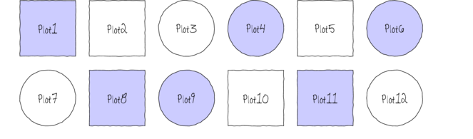
The following diagram depicts a very simple factorial design in which there are two factors (Shape and Color) each with two levels (Shape: square and circle; Color: blue and white) and each combination has 3 replicates.

In addition to investigating the impacts of the main factors, factorial designs allow us to investigate whether the effects of one factor are consistent across levels of another factor. For example, is the effect of temperature on growth rate the same for both fertilized and unfertilized seedlings and similarly, does the impact of fertilizer treatment depend on the temperature under which the seedlings are grown?

Arguably, these interactions give more sophisticated insights into the dynamics of the system we are investigating. Hence, we could add additional main effects, such as soil pH, amount of water etc along with all the two way (temp:fert, temp:pH, temp:water, etc), three-way (temp:fert:pH, temp:pH:water), four-way etc interactions in order to explore how these various factors interact with one another to effect the response.

However, the more interactions, the more complex the model becomes to specify, compute and interpret - not to mention the rate at which the number of required observations increases.

To appreciate the interpretation of interactions, consider the following figure that depicts fictitious two factor (temperature and fertilizer) designs.

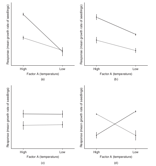
It is clear from the top-right figure that whether or not there is an observed effect of adding fertilizer or not depends on whether we are focused on seedlings growth under high or low temperatures. Fertilizer is only important for seedlings grown under high temperatures. In this case, it is not possible to simply state that there is an effect of fertilizer as it depends on the level of temperature. Similarly, the magnitude of the effect of temperature depends on whether fertilizer has been added or not.

Such interactions are represented by plots in which lines either intersect or converge. The top-right and bottom-left figures both depict parallel lines which are indicative of no interaction. That is, the effects of temperature are similar for both fertilizer added and controls and vice verse. Whilst the former displays an effect of both fertilizer and temperature, the latter only fertilizer is important.

Finally, the bottom-right figure represents a strong interaction that would mask the main effects of temperature and fertilizer (since the nature of the effect of temperature is very different for the different fertilizer treatments and visa verse).

Factorial designs can consist:

entirely of crossed fixed factors (Model I ANOVA - most common) in which conclusions are restricted to the specific combinations of levels selected for the experiment,
entirely of crossed random factors (Model II ANOVA) or
a mixture of crossed fixed and random factors (Model III ANOVA).

The latter are useful for investigating the generality of a main treatment effect (fixed) over broad spatial, temporal or biological levels of organization. That is whether the observed effects of temperature and/or fertilizer (for example) are observed across the entire genera or country.

Linear model

As with single factor ANOVA, the linear model could be constructed as either effects or cell means parameterization, although only effects parameterization will be considered here (as cell means parameterization is of little use in frequentist factorial ANOVA).

The linear models for two and three factor design are: $$y_{ijk}=\mu+\alpha_i + \beta_{j} + (\alpha\beta)_{ij} + \varepsilon_{ijk}$$ $$y_{ijkl}=\mu+\alpha_i + \beta_{j} + \gamma_{k} + (\alpha\beta)_{ij} + (\alpha\gamma)_{ik} + (\beta\gamma)_{jk} + (\alpha\beta\gamma)_{ijk} + \varepsilon_{ijkl}$$ where $\mu$ is the overall mean, $\alpha$ is the effect of Factor A, $\beta$ is the effect of Factor B, $\gamma$ is the effect of Factor C and $\varepsilon$ is the random unexplained or residual component.

Note that although the linear models for Model I, Model II and Model III designs are identical, the interpretation of terms (and thus null hypothesis) differ.

Recall from the tutorial on single factor ANOVA, that categorical variables in linear models are actually re-parameterized dummy codes - and thus the $\alpha$ term above, actually represents one or more dummy codes. Thus, if we actually had two levels of Factor A (A1 and A2) and three levels of Factor B (B1, B2, B3), then the fully parameterized linear model would be: $$y = \beta_{A1B1} + \beta_{A2B1 - A1B1} + \beta_{A1B2 - A1B1} + \beta_{A1B3 - A1B1} + \beta_{A2B2 - A1B2 - A2B1 - A1B1} + \beta_{A2B3 - A1B3 - A2B1 - A1B1}$$ Thus, such a model would have six parameters to estimate (in addition to the variance).

Null hypotheses

There are separate null hypothesis associated with each of the main effects and the interaction terms.

Model 1 - fixed effects

Factor A

H$_0(A)$: $\mu_1=\mu_2=...=\mu_i=\mu$ (the population group means are all equal).

The mean of population 1 is equal to that of population 2 and so on, and thus all population means are equal to an overall mean. If the effect of the $i^{th}$ group is the difference between the $i^{th}$ group mean and the overall mean ($\alpha_i = \mu_i - \mu$) then the H$_0$ can alternatively be written as:
H$_0(A)$: $\alpha_1 = \alpha_2 = ... = \alpha_i = 0$ (the effect of each group equals zero).

If one or more of the $\alpha_i$ are different from zero (the response mean for this treatment differs from the overall response mean), the null hypothesis is rejected indicating that the treatment has been found to affect the response variable.

Note, as with multiple regression models, these "effects" represent partial effects. In the above, the effect of Factor A is actually the effect of Factor A at the first level of the Factor(s).

Factor B

H$_0(B)$: $\mu_1=\mu_2=...=\mu_i=\mu$ (the population group means are all equal - at the first level of Factor A).

Equivalent interpretation to Factor A above.

A: Interaction

H$_0(AB)$: $\mu_{ij}=\mu_i+\mu_j-\mu$ (the population group means are all equal).

For any given combination of factor levels, the population group mean will be equal to the difference between the overall population mean and the simple additive effects of the individual factor group means. That is, the effects of the main treatment factors are purely additive and independent of one another. This is equivalent to H$_0(AB)$: $\alpha\beta_{ij}=0$, no interaction between Factor A and Factor B.

Model 2 - random effects

Factor A

H$_0(A)$: $\sigma_\alpha^2=0$ (population variance equals zero)

There is no added variance due to all possible levels of A.

Factor B

H$_0(B)$: $\sigma_\alpha^2=0$ (population variance equals zero)

There is no added variance due to all possible levels of B.

A:B Interaction

H$_0(AB)$: $\sigma_{\alpha \beta}^2=0$ (population variance equals zero)

There is no added variance due to all possible interactions between all possible levels of A and B.

Model 3 - mixed effects

Fixed factor - e.g. A

H$_0(A)$: $\mu_1=\mu_2=...=\mu_i=\mu$ (the population group means are all equal)

The mean of population 1 (pooled over all levels of the random factor) is equal to that of population 2 and so on, and thus all population means are equal to an overall mean pooling over all possible levels of the random factor. If the effect of the $i^{th}$ group is the difference between the $i^{th}$ group mean and the overall mean ($\alpha_i = \mu_i - \mu$) then the H$_0$ can alternatively be written as:
H$_0(A)$: $\alpha_1 = \alpha_2 = ... = \alpha_i = 0$ (no effect of any level of this factor pooled over all possible levels of the random factor)

Random factor - e.g. B

H$_0(B)$: $\sigma_\alpha^2=0$ (population variance equals zero)

There is no added variance due to all possible levels of B.

A:B Interaction

The interaction of a fixed and random factor is always considered a random factor.
H$_0(AB)$: $\sigma_{\alpha \beta}^2=0$ (population variance equals zero)

There is no added variance due to all possible interactions between all possible levels of A and B.

Analysis of Variance

When fixed factorial designs are balanced, the total variance in the response variable can be sequentially partitioned into what is explained by each of the model terms (factors and their interactions) and what is left unexplained. For each of the specific null hypotheses, the overall unexplained variability is used as the denominator in F-ratio calculations (see tables below), and when a null hypothesis is true, an ,F-ratio should follow an F distribution with an expected value less than 1.

Random factors are added to provide greater generality of conclusions. That is, to enable us to make conclusions about the effect of one factor (such as whether or not fertilizer is added) over all possible levels (not just those sampled) of a random factor (such as all possible locations, seasons, varieties etc). In order to expand our conclusions beyond the specific levels used in the design, the hypothesis tests (and thus F-ratios) must reflect this extra generality by being more conservative.

The appropriate F-ratios for fixed, random and mixed factorial designs are presented in tables below. Generally, once the terms (factors and interactions) have been ordered into a hierarchy (single factors at the top, highest level interactions at the bottom and terms of same order given equivalent positions in the hierarchy), the denominator for any term is selected as the next appropriate random term (an interaction that includes the term to be tested) encountered lower in the hierarchy. Interaction terms that contain one or more random factors are considered themselves to be random terms, as is the overall residual term (as all observations are assumed to be random representations of the entire population(s)).

Note, when designs include a mixture of fixed and random crossed effects, exact denominator degrees of freedoms for certain F-ratios are undefined and traditional approaches adopt rather inexact estimated approximate or "Quasi" F-ratios.

Pooling of non-significant F-ratio denominator terms, in which lower random terms are added to the denominator (provided $\alpha\gt 0.25$), may also be useful.

For random factors within mixed models, selecting F-ratio denominators that are appropriate for the intended hypothesis tests is a particularly complex and controversial issue. Traditionally, there are two alternative approaches and whilst the statistical resumes of each are complicated, essentially they differ in whether or not the interaction term is constrained for the test of the random factor.

The constrained or restricted method (Model I), stipulates that for the calculation of a random factor F-ratio (which investigates the added variance added due to the random factor), the overall effect of the interaction is treated as zero. Consequently, the random factor is tested against the residual term (see tables below).

The unconstrained or unrestrained method (Model II) however, does not set the interaction effect to zero and therefore the interaction term is used as the random factor F-ratio denominator (see tables below). This method assumes that the interaction terms for each level of the random factor are completely independent (correlations between the fixed factor must be consistent across all levels of the random factor).

Some statisticians maintain that the independence of the interaction term is difficult to assess for biological data and therefore, the restricted approach is more appropriate. However, others have suggested that the restricted method is only appropriate for balanced designs.

Quasi F-ratios

An additional complication for three or more factor models that contain two or more random factors, is that there may not be a single appropriate interaction term to use as the denominator for many of the main effects F-ratios. For example, if Factors A and B are random and C is fixed, then there are two random interaction terms of equivalent level under Factor C (A$^{\prime}\times$C and B$^{\prime}\times$C).

As a result, the value of the of the Mean Squares expected when the null hypothesis is true cannot be easily defined. The solutions for dealing with such situations (quasi F-ratios involve adding (and subtracting) terms together to create approximate estimates of F-ratio denominators. Alternatively, for random factors, variance components with confidence intervals can be used.)

These solutions are sufficiently unsatisfying as to lead many biostatisticians to recommend that factorial designs with two or more random factors should avoided if possible. Arguably however, linear mixed effects models offer more appropriate solutions to the above issues as they are more robust for unbalanced designs, accommodate covariates and provide a more comprehensive treatment and overview of all the underlying data structures.

					A fixed, B random
Factor	d.f	MS	A,B fixed	A,B random	Restricted	Unrestricted
A	$a-1$	$MS_A$	$MS_A/MS_{Resid}$	$MS_A/MS_{A:B}$	$MS_A/MS_{A:B}$	$MS_A/MS_{A:B}$
B	$b-1$	$MS_B$	$MS_B/MS_{Resid}$	$MS_B/MS_{A:B}$	$MS_B/MS_{Resid}$	$MS_B/MS_{A:B}$
A:B	$(b-1)(a-1)$	$MS_{A:B}$	$MS_{A:B}/MS_{Resid}$	$MS_{A:B}/MS_{A:B}$	$MS_{A:B}/MS_{Resid}$	$MS_{A:B}/MS_{Resid}$
Residual (=$N^{\prime}(B:A)$)	$(n-1)ba$	$MS_{Resid}$
		*R syntax*
Type I SS (Balanced)		summary(lm(y ~ A * B, data)) anova(lm(y ~ A * B, data))
Type II SS (Unbalanced)		summary(lm(y ~ A * B, data)) library(car) Anova(lm(y ~ A * B, data), type = "II")
Type III SS (Unbalanced)		summary(lm(y ~ A * B, data)) library(car) contrasts(data$A) <- contr.sum contrasts(data$B) <- contr.sum Anova(lm(y ~ A * B, data), type = "III")
Variance components		library(lme4) summary(lmer(y ~ 1 + (1 \| A) + (1 \| B) + (1 \| A:B), data))

Interactions and main effects tests

Note that for fixed factor models, when null hypotheses of interactions are rejected, the null hypothesis of the individual constituent factors are unlikely to represent the true nature of the effects and thus are of little value.

The nature of such interactions are further explored by fitting simpler linear models (containing at least one less factor) separately for each of the levels of the other removed factor(s). Such Main effects tests are based on a subset of the data, and therefore estimates of the overall residual (unexplained) variability are unlikely to be as precise as the estimates based on the global model. Consequently, F-ratios involving $MS_{Resid}$ should use the estimate of $MS_{Resid}$ from the global model rather than that based on the smaller, theoretically less precise subset of data.

For random and mixed models, since the objective is to generalize the effect of one factor over and above any interactions with other factors, the main factor effects can be interpreted even in the presence of significant interactions. Nevertheless, it should be noted that when a significant interaction is present in a mixed model, the power of the main fixed effects will be reduced (since the amount of variability explained by the interaction term will be relatively high, and this term is used as the denominator for the F-ratio calculation).

Assumptions

Hypothesis tests assume that the residuals are:

normally distributed. Boxplots using the appropriate scale of replication (reflecting the appropriate residuals/F-ratio denominator (see table above) should be used to explore normality. Scale transformations are often useful.
equally varied. Boxplots and plots of means against variance (using the appropriate scale of replication) should be used to explore the spread of values. Residual plots should reveal no patterns. Scale transformations are often useful.
independent of one another.

Planned and unplanned comparisons

As with single factor analysis of variance, planned and unplanned multiple comparisons (such as Tukey's test) can be incorporated into or follow the linear model respectively so as to further investigate any patterns or trends within the main factors and/or the interactions. As with single factor analysis of variance, the contrasts must be defined prior to fitting the linear model, and no more than $p-1$ (where $p$ is the number of levels of the factor) contrasts can be defined for a factor.

Unbalanced designs

A factorial design can be thought of as a table made up of rows (representing the levels of one factor), columns (levels of another factor) and cells (the individual combinations of the set of factors), see the series of tables below. The top two tables depict a balanced two factor (3x3) design in which each cell (combination of factor levels) has three replicate observation.

Whilst the middle left table does not have equal sample sizes in each cell, the sample sizes are in proportion and as such, does not present the issues discussed below for unbalanced designs.

Tables middle-right and bottom-left are considered unbalanced as is the bottom-right (which is a special case in which the entire cell is missing).

Cell means structure

	High	Medium	Low
Full shade	$\mu_{FH}$	$\mu_{FM}$	$\mu_{FL}$
Partial shade	$\mu_{PH}$	$\mu_{PM}$	$\mu_{PL}$
Control	$\mu_{CH}$	$\mu_{CM}$	$\mu_{CL}$

Balanced design (3 replicates)

	High	Medium	Low
Full shade	XXX	XXX	XXX
Partial shade	XXX	XXX	XXX
Control	XXX	XXX	XXX

Proportionally balanced design (2-3 replicates)

	High	Medium	Low
Full shade	XXX	XXX	XXX
Partial shade	XX	XX	XX
Control	XXX	XXX	XXX

Unbalanced design (2-3 replicates)

	High	Medium	Low
Full shade	XX	XXX	XXX
Partial shade	XXX	XXX	XXX
Control	XXX	XXX	XXX

Unbalanced design (1-3 replicates)

	High	Medium	Low
Full shade	XX	XXX	XXX
Partial shade	XXX	X	XX
Control	XXX	XXX	XXX

Missing cells design (3 replicates)

	High	Medium	Low
Full shade	XXX	XXX
Partial shade	XXX	XXX	XXX
Control	XXX	XXX	XXX

Missing observations

In addition to impacting on normality and homogeneity of variance, unequal sample sizes in factorial designs have major implications for the partitioning of the total sums of squares into each of the model components.

For balanced designs, the total sums of squares ($SS_{Total}$) is equal to the additive sums of squares of each of the components (including the residual). For example, in a two factor balanced design, $SS_{Total} = SS_A + SS_B + SS_{AB} + SS_{Resid}$. This can be represented diagrammatically by a Venn Diagram in which each of the $SS$ for the term components butt against one another and are surrounded by the $SS_{Resid}$ (see the top-right figure below).

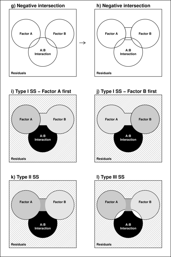
However, in unbalanced designs, the sums of squares will be non-orthogonal and the sum of the individual components does not add up to the total sums of squares. Diagrammatically, the SS of the terms intersect or are separated (see~Figure~\ref{fig:factorialInteractionPlot}b and \ref{fig:factorialInteractionPlot}g respectively).

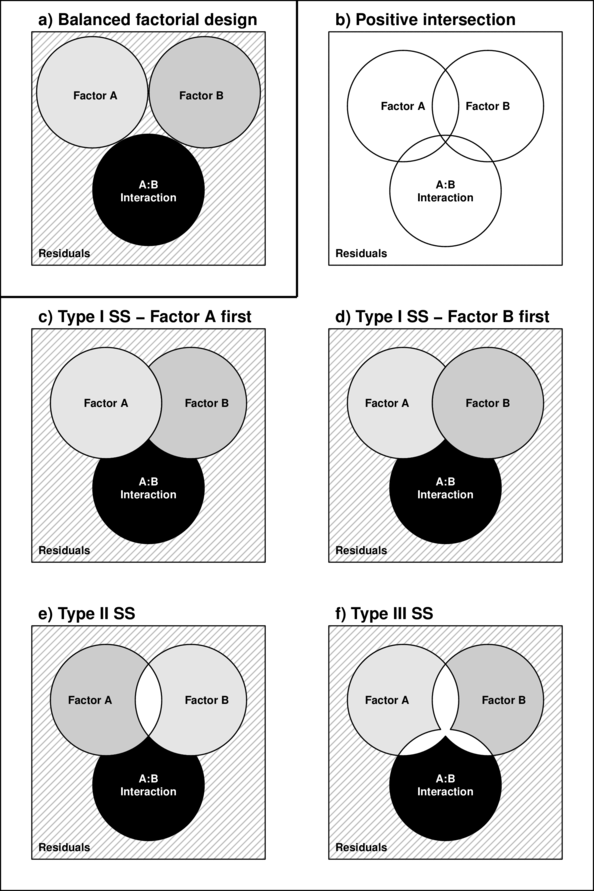
In regular sequential sums of squares (Type I SS), the sum of the individual sums of squares must be equal to the total sums of squares, the sums of squares of the last factor to be estimated will be calculated as the difference between the total sums of squares and what has already been accounted for by other components.

Consequently, the order in which factors are specified in the model (and thus estimated) will alter their sums of squares and therefore their F-ratios (see~sub-figures c-d above).

To overcome this problem, traditionally there are two other alternative methods of calculating sums of squares.

Type II (hierarchical) SS estimate the sums of squares of each term as the improvement it contributes upon addition of that term to a model of greater complexity and lower in the hierarchy (recall that the hierarchical structure descends from the simplest model down to the fully populated model). The SS for the interaction as well as the first factor to be estimated are the same as for Type I SS. Type II SS estimate the contribution of a factor over and above the contributions of other factors of equal or lower complexity but not above the contributions of the interaction terms or terms nested within the factor. However, these sums of squares are weighted by the sample sizes of each level and therefore are biased towards the trends produced by the groups (levels) that have higher sample sizes. As a result of the weightings, Type II SS actually test hypotheses about really quite complex combinations of factor levels. Rather than test a hypothesis that $\mu_{High}=\mu_{Medium}=\mu{Low}$, Type II SS might be testing that $4\times\mu_{High}=1\times\mu_{Medium}=0.25\times\mu{Low}$.
Type III (marginal or orthogonal) SS estimate the sums of squares of each term as the improvement based on a comparison of models with and without the term and are unweighted by sample sizes. Type III SS essentially measure just the unique contribution of each factor over and above the contributions of the other factors and interactions. For unbalanced designs,Type III SS essentially test equivalent hypotheses to balanced Type I SS and are therefore arguably more appropriate for unbalanced factorial designs than Type II SS. Importantly, Type III SS are only interpretable if they are based on orthogonal contrasts (such as sum or helmert contrasts and not treatment contrasts).

The choice between Type II and III SS clearly depends on the nature of the question. For example, if we had measured the growth rate of seedlings subjected to two factors (temperature and fertilizer), Type II SS could address whether there was an effect of temperature across the level of fertilizer treatment, whereas Type III SS could assess whether there was an effect of temperature within each level of the fertilizer treatment.

Missing cells

When an entire combination, or cell, is missing (perhaps due to unforeseen circumstances) it is not possible to test all the main effects and/or interactions. The bottom right table above depicts such as situation.

One solution is to fit a large single factor ANOVA with as many levels as there are cells (this is known as a cell means model) and investigate various factor and interaction effects via specific contrasts (see the following tables). Difficulties in establishing appropriate error terms, makes missing cells in random and mixed factor designs substantially more complex.

ANOVA in R

Scenario and Data

Imagine we has designed an experiment in which we had measured the response ($y$) under a combination of two different potential influences (Factor A: levels $a1$ and $a2$; and Factor B: levels $b1$, $b2$ and $b3$), each combination replicated 10 times ($n=10$). As this section is mainly about the generation of artificial data (and not specifically about what to do with the data), understanding the actual details are optional and can be safely skipped. Consequently, I have folded (toggled) this section away.

Details of data generation

Random data incorporating the following trends (effect parameters)

the sample size per treatment=10
factor A with 2 levels
factor B with 3 levels
the 6 effects parameters are 40, 15, 5, 0, -15,10 ($\mu_{a1b1}=40$, $\mu_{a2b1}=40+15=55$, $\mu_{a1b2}=40+5=45$, $\mu_{a1b3}=40+0=40$, $\mu_{a2b2}=40+15+5-15=45$ and $\mu_{a2b3}=40+15+0+10=65$)
the data are drawn from normal distributions with a mean of 0 and standard deviation of 3 ($\sigma^2=9$)

set.seed(1)
nA <- 2  #number of levels of A
nB <- 3  #number of levels of B
nsample <- 10  #number of reps in each
A <- gl(nA, 1, nA, lab = paste("a", 1:nA, sep = ""))
B <- gl(nB, 1, nB, lab = paste("b", 1:nB, sep = ""))
data <- expand.grid(A = A, B = B, n = 1:nsample)
X <- model.matrix(~A * B, data = data)
eff <- c(40, 15, 5, 0, -15, 10)
sigma <- 3  #residual standard deviation
n <- nrow(data)
eps <- rnorm(n, 0, sigma)  #residuals
data$y <- as.numeric(X %*% eff + eps)
head(data)  #print out the first six rows of the data set

   A  B n        y
1 a1 b1 1 38.12064
2 a2 b1 1 55.55093
3 a1 b2 1 42.49311
4 a2 b2 1 49.78584
5 a1 b3 1 40.98852
6 a2 b3 1 62.53859

with(data, interaction.plot(A, B, y))

## ALTERNATIVELY, we could supply the population means and get the effect parameters from these.  To
## correspond to the model matrix, enter the population means in the order of: a1b1, a2b1, a1b1,
## a2b2,a1b3,a2b3
pop.means <- as.matrix(c(40, 55, 45, 45, 40, 65), byrow = F)
## Generate a minimum model matrix for the effects
XX <- model.matrix(~A * B, expand.grid(A = factor(1:2), B = factor(1:3)))
## Use the solve() function to solve what are effectively simultaneous equations
(eff <- as.vector(solve(XX, pop.means)))

[1]  40  15   5   0 -15  10

data$y <- as.numeric(X %*% eff + eps)

Exploratory data analysis

Normality and Homogeneity of variance

boxplot(y ~ A * B, data)

library(ggplot2)
ggplot(data, aes(y = y, x = A, fill = B)) + geom_boxplot()

Conclusions:

there is no evidence that the response variable is consistently non-normal across all populations - each boxplot is approximately symmetrical
there is no evidence that variance (as estimated by the height of the boxplots) differs between the five populations. . More importantly, there is no evidence of a relationship between mean and variance - the height of boxplots does not increase with increasing position along the y-axis. Hence it there is no evidence of non-homogeneity

Obvious violations could be addressed either by:

transform the scale of the response variables (to address normality etc). Note transformations should be applied to the entire response variable (not just those populations that are skewed).

Model fitting or statistical analysis

In R, simple ANOVA models (being regression models) are fit using the lm() function. The most important (=commonly used) parameters/arguments for simple regression are:

formula: the linear model relating the response variable to the linear predictor
data: the data frame containing the data

data.lm <- lm(y ~ A * B, data)

Model evaluation

Prior to exploring the model parameters, it is prudent to confirm that the model did indeed fit the assumptions and was an appropriate fit to the data.

Whilst ANOVA models are multiple regression models, some of the regression usual diagnostics are not relevant. For example, an observation cannot logically be an outlier in x-space - it must be in one of the categories. In this case, each observation comes from one of five treatment groups. No observation can be outside of these categories and thus there are no opportunities for outliers in x-space. Consequently, Leverage (and thus Cook's D) diagnostics have no real meaning in ANOVA.

Residuals

As the residuals are the differences between the observed and predicted values along a vertical plane, they provide a measure of how much of an outlier each point is in y-space (on y-axis). Outliers are identified by relatively large residual values. Residuals can also standardized and studentized, the latter of which can be compared across different models and follow a t distribution enabling the probability of obtaining a given residual can be determined. The patterns of residuals against predicted y values (residual plot) are also useful diagnostic tools for investigating linearity and homogeneity of variance assumptions.

par(mfrow = c(2, 2))
plot(data.lm)

Conclusions:

there are no obvious patterns in the residuals (top-left plot). Specifically, there is no obvious 'wedge-shape' suggesting that we still have no evidence of non-homogeneity of variance
Whilst the data do appear to deviate slightly from normality according to the Q-Q normal plot, it is only a mild deviation and given the robustness of linear models to mild non-normality, the Q-Q normal plot is really only of interest when there is also a wedge in the residuals (as it could suggest that non-homogeneity of variance could be due to non-normality and that perhaps normalizing could address both issues).
The lower-left figure is a re-representation of the residual plot (yet with standardized residuals - hence making it more useful when the model has applied alternate variance structures) and therefore don't provide any additional insights if the default variance structure is applied.
The lower-right figure represents the residuals for each combination of levels of the two factors. In examining this figure, we are looking to see whether the spread of the residuals is similar for each factor combination - which it is.

Extractor functions

There are a number of extractor functions (functions that extract or derive specific information from a model) available including:

Extractor	Description
`residuals()`	Extracts the residuals from the model
`fitted()`	Extracts the predicted (expected) response values (on the link scale) at the observed levels of the linear predictor
`predict()`	Extracts the predicted (expected) response values (on either the link, response or terms (linear predictor) scale)
`coef()`	Extracts the model coefficients
`confint()`	Calculate confidence intervals for the model coefficients
`summary()`	Summarizes the important output and characteristics of the model
`anova()`	Computes an analysis of variance (variance partitioning) from the model
`plot()`	Generates a series of diagnostic plots from the model
`effect()`	effects package - estimates the marginal (partial) effects of a factor (useful for plotting)
`avPlot()`	car package - generates partial regression plots

Exploring the model parameters, test hypotheses

If there was any evidence that the assumptions had been violated, then we would need to reconsider the model and start the process again. In this case, there is no evidence that the test will be unreliable so we can proceed to explore the test statistics.

There are two broad hypothesis testing perspectives we could take:

We could explore the individual effects. By default, the lm() function dummy codes the categorical variable for treatment contrasts (where each of the groups are compared to the first group). These parameter estimates are best viewed in conjunction with an interaction plot.

summary(data.lm)

Call:
lm(formula = y ~ A * B, data = data)

Residuals:
    Min      1Q  Median      3Q     Max 
-7.3944 -1.5753  0.2281  1.5575  5.1909 

Coefficients:
            Estimate Std. Error t value Pr(>|t|)    
(Intercept)  41.0988     0.8218  50.010  < 2e-16 ***
Aa2          14.6515     1.1622  12.606  < 2e-16 ***
Bb2           4.6386     1.1622   3.991   0.0002 ***
Bb3          -0.7522     1.1622  -0.647   0.5202    
Aa2:Bb2     -15.7183     1.6436  -9.563 3.24e-13 ***
Aa2:Bb3       9.3352     1.6436   5.680 5.54e-07 ***
---
Signif. codes:  0 '***' 0.001 '**' 0.01 '*' 0.05 '.' 0.1 ' ' 1

Residual standard error: 2.599 on 54 degrees of freedom
Multiple R-squared:  0.9245,	Adjusted R-squared:  0.9175 
F-statistic: 132.3 on 5 and 54 DF,  p-value: < 2.2e-16

library(effects)
plot(effect("A:B", data.lm))

plot of chunk tut7.6aS3.1InteractionPlot

library(car)
with(data, interaction.plot(B, A, y))

Conclusions:

The row in the Coefficients table labeled (Intercept) represents the first combination of treatment groups. So the Estimate for this row represents the estimated population mean for a1b1). Hence, the mean of population a1b1 (Factor A level 1 and Factor B level 1) is estimated to be 41.099 with a standard error (precision) of 0.822. Note that the rest of the columns (t value and Pr(>|t|))represent the outcome of hypothesis tests. For the first row, this hypothesis test has very little meaning as it is testing the null hypothesis that the mean of population A is zero.
Each of the subsequent rows represent the estimated effects of each of the other population combinations from population a1b1. For example, the Estimate for the row labeled Aa2 represents the estimated difference in means between a2b1 and the reference group (a1b1). Hence, the population mean of a2b1 is estimated to be 14.651 units higher than the mean of a1b1 and this 'effect' is statistically significant (at the 0.05 level).
This can be seen visually in the interaction plot, where the mean of a1b1 is approximately 41 and the mean of a1b1 is approximately 55.5 (i.e. approx. 14.5 units higher).
Similarly, a1b2 and a1b3 represent the differences in their respective means (approx 4.639 and -0.752) from the mean on a1b1.
So far, those estimates indicate that the "effect" of Factor B is that the response increases slightly between b1 and b2 before returning down again by b3. The "effect" of Factor A suggests that a2 is approximately 15 units greater than a1. However, these are partial effects. It is clear, that the patterns described between b1,b2 and b3 are only appropriate for a1. The patterns between b1, b2 and b3 are very different for b2.
The last two parameters (rows of the table), indicate the deviations of the patterns in additional levels of each factor are from the partial effects suggested by e main terms (A and B). The item Aa2:Bb2 is the deviation of mean a2b2 from what would be expected based on the deviations of a2b1 and a1b2 from a1b1. For example, we know that a1b2 is 4.639 units higher than a1b2 and we know that a2b1 is 14.651 units higher than a1b2. So if the model was purely additive (no interaction), we would expect the mean of a2b2 would be approximately 60.389. And Aa2:Bb2 would equal 0.
The value of Aa2:Bb2 of -15.718 indicates that a2b2 is considerably less than 0. So interaction terms, the effects of b2-b1 are considerably stronger (larger magnitude) at a2 than they are at a1.
The $R^2$ value is 0.92 suggesting that approximately 92% of the total variance in $y$ can be explained by the multiplicative model. The $R^2$ value is thus a measure of the strength of the relationship.
Alternatively, we could calculate the 95% confidence intervals for the parameter estimates.
confint(data.lm)
2.5 % 97.5 % (Intercept) 39.451199 42.746488 Aa2 12.321368 16.981611 Bb2 2.308462 6.968705 Bb3 -3.082360 1.577884 Aa2:Bb2 -19.013589 -12.423010 Aa2:Bb3 6.039883 12.630463

In addition (or alternatively), we could explore the collective null hypothesis (that all the population means are equal) by partitioning the variance into explained and unexplained components (in an ANOVA table). Since the design was balanced, we can use regular Type I SS.
anova(data.lm)
Analysis of Variance Table Response: y Df Sum Sq Mean Sq F value Pr(>F) A 1 2352.68 2352.68 348.346 < 2.2e-16 *** B 2 510.82 255.41 37.817 5.385e-11 *** A:B 2 1603.14 801.57 118.684 < 2.2e-16 *** Residuals 54 364.71 6.75 --- Signif. codes: 0 '***' 0.001 '**' 0.01 '*' 0.05 '.' 0.1 ' ' 1
Conclusions:
- When an interaction term is present, it is important that these term(s) be looked at first (starting with the highest level interaction term). In this case, there is a single interaction term (A:B). There is clear interential evidence of an interaction between Factor A and B, suggesting (as we have already seen) that the effect on Factor A on the response is not consistent across all levels of Factor B and vice verse.
  It should be fairly evident that making any conclusions about the main effects (in the presence of a significant interaction), is missleading and well short of the full complexity of the situation.
- If the interaction term was non-significant, then we could proceed to draw conclusions about the main effects of Factor A and B as we would then effectively have an additive model (no interaction). On that note, some argue that if the interaction term has a p-value $\gt 0.25$, then the term can be removed from the model. The interaction term uses up (in this case) 2 degrees of freedom (that would otherwise be in the residuals). If the interaction term is not explaining much (and thus absorbing unexplained variability from the residuals, whilst incurring a cost of degrees of freedom), then the tests of main effects will be more powerful if the interaction is removed.

Dealing with interactions

In the current working example, we have identified that there is a significant interaction between Factor A and Factor B. Our exploration of the regression coefficients (from the summary() function, indicated that the pattern between b1, b2 and b3 might differ between a1 and a2.

Similarly, if we consider the coefficients from the perspective of Factor A (and again an interaction plot might help), we can see that the patterns between a1 and a2 are similar for b1 and b3, yet very different for b2.

library(effects)
plot(effect("A:B", data.lm))

library(car)
with(data, interaction.plot(B, A, y))

library(car)
with(data, interaction.plot(A, B, y))

plot of chunk tut7.6aS3.1InteractionPlot2

At this point, we can then split the two-factor model up into a series of single-factor ANOVA models, either:

examining the effects of Factor B separately for each level of Factor A (two single-factor ANOVA'S) or
examining the effects of Factor A separately for each level of Factor B (three single-factor ANOVA's)

When doing so, it is often considered appropriate to use the global residual term as the residual term. Hence we run the single-factor ANOVA's (main effects tests) and then modify the residual term as well as the F-ratio and P-value to reflect this.

There are three ways of performing such simple main effects tests:

Perform simple one-way ANOVA's on subsets of data and manually adjust the F-ratios and P values
Refit the model including a new modified interaction term designed to capture the other levels of one of the factors. This option can then generate the new regression coefficients as well as the ANOVA table.
Apply a specific contrast. This approach only generates the new regression coefficients (and associated inference tests)

Manual adjustments
I will only demonstrate exploring the effects of Factor A at b1 and b2 as an example.

## Examine the effects of Factor A at level b1 of Factor B
summary(lm(y ~ A, data = subset(data, B == "b1")))

Call:
lm(formula = y ~ A, data = subset(data, B == "b1"))

Residuals:
   Min     1Q Median     3Q    Max 
-7.394 -1.153  0.562  1.390  5.191 

Coefficients:
            Estimate Std. Error t value Pr(>|t|)    
(Intercept)   41.099      0.881   46.65  < 2e-16 ***
Aa2           14.652      1.246   11.76 6.98e-10 ***
---
Signif. codes:  0 '***' 0.001 '**' 0.01 '*' 0.05 '.' 0.1 ' ' 1

Residual standard error: 2.786 on 18 degrees of freedom
Multiple R-squared:  0.8848,	Adjusted R-squared:  0.8784 
F-statistic: 138.3 on 1 and 18 DF,  p-value: 6.984e-10

anova(lm(y ~ A, data = subset(data, B == "b1")))

Analysis of Variance Table

Response: y
          Df Sum Sq Mean Sq F value    Pr(>F)    
A          1 1073.3 1073.33  138.29 6.984e-10 ***
Residuals 18  139.7    7.76                      
---
Signif. codes:  0 '***' 0.001 '**' 0.01 '*' 0.05 '.' 0.1 ' ' 1

## Use global MSresid instead
(MS_A <- anova(lm(y ~ A, data = subset(data, B == "b1")))$"Mean Sq"[1])

[1] 1073.331

(DF_A <- anova(lm(y ~ A, data = subset(data, B == "b1")))$Df[1])

[1] 1

(MS_resid <- anova(data.lm)$"Mean Sq"[4])

[1] 6.753839

(DF_resid <- anova(data.lm)$Df[4])

[1] 54

(F_ratio <- MS_A/MS_resid)

[1] 158.9216

(P_value <- 1 - pf(F_ratio, DF_A, DF_resid))

[1] 0

## Examine the effects of Factor A at level b2 of Factor B
summary(lm(y ~ A, data = subset(data, B == "b2")))

Call:
lm(formula = y ~ A, data = subset(data, B == "b2"))

Residuals:
    Min      1Q  Median      3Q     Max 
-4.0829 -1.8046  0.1813  2.1553  5.1152 

Coefficients:
            Estimate Std. Error t value Pr(>|t|)    
(Intercept)  45.7374     0.7916  57.777   <2e-16 ***
Aa2          -1.0668     1.1195  -0.953    0.353    
---
Signif. codes:  0 '***' 0.001 '**' 0.01 '*' 0.05 '.' 0.1 ' ' 1

Residual standard error: 2.503 on 18 degrees of freedom
Multiple R-squared:  0.04803,	Adjusted R-squared:  -0.004862 
F-statistic: 0.9081 on 1 and 18 DF,  p-value: 0.3533

anova(lm(y ~ A, data = subset(data, B == "b2")))

Analysis of Variance Table

Response: y
          Df Sum Sq Mean Sq F value Pr(>F)
A          1   5.69  5.6904  0.9081 0.3533
Residuals 18 112.80  6.2665

## Use global MSresid instead
(MS_A <- anova(lm(y ~ A, data = subset(data, B == "b2")))$"Mean Sq"[1])

[1] 5.69042

(DF_A <- anova(lm(y ~ A, data = subset(data, B == "b2")))$Df[1])

[1] 1

(MS_resid <- anova(data.lm)$"Mean Sq"[4])

[1] 6.753839

(DF_resid <- anova(data.lm)$Df[4])

[1] 54

(F_ratio <- MS_A/MS_resid)

[1] 0.8425459

(P_value <- 1 - pf(F_ratio, DF_A, DF_resid))

[1] 0.3627514

There is a clear evidence of an effect of Factor A at level b1, yet no evidence of an effect of Factor A at b2.

Refit the model with modified interaction term

data <- within(data, {
    A2 = ifelse(B == "b1", "a1", as.character(A))
})
data <- within(data, {
    AB = interaction(A2, B)
})
anova(update(data.lm, ~AB + .))

Analysis of Variance Table

Response: y
          Df Sum Sq Mean Sq F value    Pr(>F)    
AB         4 3393.3  848.33  125.61 < 2.2e-16 ***
A          1 1073.3 1073.33  158.92 < 2.2e-16 ***
Residuals 54  364.7    6.75                      
---
Signif. codes:  0 '***' 0.001 '**' 0.01 '*' 0.05 '.' 0.1 ' ' 1

data <- within(data, {
    A2 = ifelse(B == "b2", "a1", as.character(A))
})
data <- within(data, {
    AB = interaction(A2, B)
})
anova(update(data.lm, ~AB + .))

Analysis of Variance Table

Response: y
          Df Sum Sq Mean Sq  F value Pr(>F)    
AB         4 4461.0 1115.24 165.1265 <2e-16 ***
A          1    5.7    5.69   0.8425 0.3628    
Residuals 54  364.7    6.75                    
---
Signif. codes:  0 '***' 0.001 '**' 0.01 '*' 0.05 '.' 0.1 ' ' 1

Same conclusion as above.

Apply specific contrasts

This process will perform three contrasts - the effect of Factor A (a2-a1) at each level of Factor B.

library(contrast)
contrast(data.lm, a = list(A = "a2", B = levels(data$B)), b = list(A = "a1", B = levels(data$B)))

lm model parameter contrast

 Contrast     S.E.     Lower     Upper     t df Pr(>|t|)
 14.65149 1.162225 12.321368 16.981611 12.61 54   0.0000
 -1.06681 1.162225 -3.396932  1.263311 -0.92 54   0.3628
 23.98666 1.162225 21.656541 26.316784 20.64 54   0.0000

Factor A level a2 is significantly higher than a1 at levels b1 and b3, yet not different at level b2.

Unbalanced designs

As mentioned earlier, unbalanced designs result in under (or over) estimates of main effects via sequential sums of Squares. To illustrate this, we will remove a couple of observations from our fabricated data set so as to yield an unbalanced design.

data1 <- data[c(-3, -6, -12), ]
with(data1, table(A, B))

    B
A    b1 b2 b3
  a1 10  9 10
  a2 10 10  8

## If the following function returns a list (implying that the number of replicates is different for
## different combinations of factors), then the design is NOT balanced
replications(~A * B, data1)

$A
A
a1 a2 
29 28 

$B
B
b1 b2 b3 
20 19 18 

$`A:B`
    B
A    b1 b2 b3
  a1 10  9 10
  a2 10 10  8

I will now fit the linear model (and summarize as an ANOVA table) twice - once with Factor A first and the second time with Factor B first.

anova(lm(y ~ A * B, data1))

Analysis of Variance Table

Response: y
          Df  Sum Sq Mean Sq F value    Pr(>F)    
A          1 2001.48 2001.48 294.659 < 2.2e-16 ***
B          2  408.26  204.13  30.052 2.382e-09 ***
A:B        2 1526.60  763.30 112.373 < 2.2e-16 ***
Residuals 51  346.42    6.79                      
---
Signif. codes:  0 '***' 0.001 '**' 0.01 '*' 0.05 '.' 0.1 ' ' 1

anova(lm(y ~ B * A, data1))

Analysis of Variance Table

Response: y
          Df  Sum Sq Mean Sq F value    Pr(>F)    
B          2  297.31  148.66  21.885 1.374e-07 ***
A          1 2112.43 2112.43 310.993 < 2.2e-16 ***
B:A        2 1526.60  763.30 112.373 < 2.2e-16 ***
Residuals 51  346.42    6.79                      
---
Signif. codes:  0 '***' 0.001 '**' 0.01 '*' 0.05 '.' 0.1 ' ' 1

Normally, the order in which terms are included is irrelevant. However, when the design is not balanced (as is the case here), the first term (last term estimated via sequential sums of squares) will be calculated as whatever is left after all other terms have been estimated. Notice that the SS etc for the terms A and B differ between the two fits. In both cases, the first term is underestimated.

Whilst in this case, it has no impact on the inferential outcomes, in other cases it can do. Note, it is only the ANOVA table that is affected by this, the estimated coefficients will be unaffected.

If the ANOVA table is required, then the appropriate way of modelling these data is:

Start off by defining strictly orthogonal contrasts (thus not treatment contrasts). Either sum, Helmert, polynomial or even user-defined contrasts are appropriate options.
contrasts(data1$A) <- contr.sum contrasts(data1$B) <- contr.sum
Fit the linear model (which will incorporate the contrasts).
data.lm1 <- lm(y ~ A * B, data = data1)

Generate the ANOVA table with Type III (marginal) sums of squares. For illustration purposes, I will generate ANOVA tables based on models fit with A first and B first to show that they come out the same.

library(car)
Anova(data.lm1, type = "III")

Anova Table (Type III tests)

Response: y
            Sum Sq Df   F value    Pr(>F)    
(Intercept) 134308  1 19772.885 < 2.2e-16 ***
A             2176  1   320.371 < 2.2e-16 ***
B              445  2    32.741 7.135e-10 ***
A:B           1527  2   112.373 < 2.2e-16 ***
Residuals      346 51                        
---
Signif. codes:  0 '***' 0.001 '**' 0.01 '*' 0.05 '.' 0.1 ' ' 1

Anova(lm(y ~ B * A, data = data1), type = "III")

Anova Table (Type III tests)

Response: y
            Sum Sq Df   F value    Pr(>F)    
(Intercept) 134308  1 19772.885 < 2.2e-16 ***
B              445  2    32.741 7.135e-10 ***
A             2176  1   320.371 < 2.2e-16 ***
B:A           1527  2   112.373 < 2.2e-16 ***
Residuals      346 51                        
---
Signif. codes:  0 '***' 0.001 '**' 0.01 '*' 0.05 '.' 0.1 ' ' 1

## OR with Type II (hierarchical) sums of squares
Anova(data.lm1, type = "II")

Anova Table (Type II tests)

Response: y
           Sum Sq Df F value    Pr(>F)    
A         2112.43  1 310.993 < 2.2e-16 ***
B          408.26  2  30.052 2.382e-09 ***
A:B       1526.60  2 112.373 < 2.2e-16 ***
Residuals  346.42 51                      
---
Signif. codes:  0 '***' 0.001 '**' 0.01 '*' 0.05 '.' 0.1 ' ' 1

Anova(lm(y ~ B * A, data = data1), type = "II")

Anova Table (Type II tests)

Response: y
           Sum Sq Df F value    Pr(>F)    
B          408.26  2  30.052 2.382e-09 ***
A         2112.43  1 310.993 < 2.2e-16 ***
B:A       1526.60  2 112.373 < 2.2e-16 ***
Residuals  346.42 51                      
---
Signif. codes:  0 '***' 0.001 '**' 0.01 '*' 0.05 '.' 0.1 ' ' 1

Graphical summaries

Graphical summaries of factorial ANOVA are an extension of single factor graphical summaries.

pred <- with(data, expand.grid(A = levels(A), B = levels(B)))
pred <- cbind(pred, predict(data.lm, newdata = pred, interval = "confidence"))
library(ggplot2)
ggplot(pred, aes(y = fit, x = as.numeric(B), shape = A, fill = A)) + geom_line() +
    geom_linerange(aes(ymin = lwr, ymax = upr)) + geom_point(aes(ymin = lwr,
    ymax = upr), size = 5) + scale_x_continuous("X", breaks = 1:3, labels = c("b1",
    "b2", "b3")) + scale_shape_manual("A", values = c(21, 16)) + scale_fill_manual("A",
    values = c("white", "black")) + theme_classic() + theme(legend.justification = c(0,
    1), legend.position = c(0, 1))

Worked Examples

ANCOVA references

Logan (2010) - Chpt 12
Quinn & Keough (2002) - Chpt 9

Two factor ANOVA

A biologist studying starlings wanted to know whether the mean mass of starlings differed according to different roosting situations. She was also interested in whether the mean mass of starlings altered over winter (Northern hemisphere) and whether the patterns amongst roosting situations were consistent throughout winter, therefore starlings were captured at the start (November) and end of winter (January). Ten starlings were captured from each roosting situation in each season, so in total, 80 birds were captured and weighed.

Download Starling data set

Format of starling.csv data files

SITUATION	MONTH	MASS	GROUP
S1	November	78	S1Nov
..	..	..	..
S2	November	78	S2Nov
..	..	..	..
S3	November	79	S3Nov
..	..	..	..
S4	November	77	S4Nov
..	..	..	..
S1	January	85	S1Jan
..	..	..	..

SITUATION	Categorical listing of roosting situations
MONTH	Categorical listing of the month of sampling.
MASS	Mass (g) of starlings.
GROUP	Categorical listing of situation/month combinations - used for checking ANOVA assumptions

Open the starling data file.

Show code

starling <- read.table("../downloads/data/starling.csv", header = T, sep = ",",
    strip.white = T)
head(starling)

  SITUATION    MONTH MASS GROUP
1        S1 November   78 S1Nov
2        S1 November   88 S1Nov
3        S1 November   87 S1Nov
4        S1 November   88 S1Nov
5        S1 November   83 S1Nov
6        S1 November   82 S1Nov

List the 3 null hypothesis being tested

Test the assumptions

by producing boxplots

(HINT) and mean vs variance plot

Show code

boxplot(MASS ~ SITUATION * MONTH, data = starling)

means <- with(starling, tapply(MASS, list(SITUATION, MONTH), mean))
vars <- with(starling, tapply(MASS, list(SITUATION, MONTH), var))
plot(means, vars, pch = 16)

Show ggplot2 code

library(ggplot2)
ggplot(starling, aes(y = MASS, x = SITUATION, fill = MONTH)) + geom_boxplot()

library(plyr)
dat <- ddply(starling, ~MONTH + SITUATION, function(x) {
    data.frame(Mean = mean(x$MASS, na.rm = TRUE), Var = var(x$MASS, na.rm = TRUE))
})
ggplot(dat, aes(y = Var, x = Mean)) + geom_point()

Is there any evidence that one or more of the assumptions are likely to be violated? (Y or N)
Is the proposed model balanced?
(Y or N)

Show code

replications(MASS ~ SITUATION * MONTH, data = starling)

      SITUATION           MONTH SITUATION:MONTH 
             20              40              10

!is.list(replications(MASS ~ SITUATION * MONTH, data = starling))

[1] TRUE

Now fit a two-factor ANOVA model (HINT)

and examine the residuals (HINT).

Show code

starling.lm <- lm(MASS ~ SITUATION * MONTH, data = starling)
# setup a 1x2 plotting device with small margins
par(mfrow = c(1, 2), oma = c(0, 0, 2, 0))
plot(starling.lm, ask = F, which = 1:2)

Any evidence of skewness or unequal variances? Any outliers? Any evidence of violations? ('Y' or 'N') .
Examine the ANOVA table

Show code

summary(starling.lm)

Call:
lm(formula = MASS ~ SITUATION * MONTH, data = starling)

Residuals:
   Min     1Q Median     3Q    Max 
  -7.4   -3.2   -0.4    2.9    9.2 

Coefficients:
                          Estimate Std. Error t value Pr(>|t|)    
(Intercept)                 90.800      1.330  68.260  < 2e-16 ***
SITUATIONS2                 -0.600      1.881  -0.319 0.750691    
SITUATIONS3                 -2.600      1.881  -1.382 0.171213    
SITUATIONS4                 -6.600      1.881  -3.508 0.000781 ***
MONTHNovember               -7.200      1.881  -3.827 0.000274 ***
SITUATIONS2:MONTHNovember   -3.600      2.660  -1.353 0.180233    
SITUATIONS3:MONTHNovember   -2.400      2.660  -0.902 0.370003    
SITUATIONS4:MONTHNovember   -1.600      2.660  -0.601 0.549455    
---
Signif. codes:  0 '***' 0.001 '**' 0.01 '*' 0.05 '.' 0.1 ' ' 1

Residual standard error: 4.206 on 72 degrees of freedom
Multiple R-squared:   0.64,	Adjusted R-squared:  0.605 
F-statistic: 18.28 on 7 and 72 DF,  p-value: 9.546e-14

anova(starling.lm)

Analysis of Variance Table

Response: MASS
                Df Sum Sq Mean Sq F value    Pr(>F)    
SITUATION        3  574.4  191.47 10.8207 5.960e-06 ***
MONTH            1 1656.2 1656.20 93.6000 1.172e-14 ***
SITUATION:MONTH  3   34.2   11.40  0.6443    0.5891    
Residuals       72 1274.0   17.69                      
---
Signif. codes:  0 '***' 0.001 '**' 0.01 '*' 0.05 '.' 0.1 ' ' 1

and fill in the following table:

Source of Variation	SS	df	MS	F-ratio	Pvalue
SITUATION
MONTH
SITUATION : MONTH
Residual (within groups)

An interaction plot (plot of means)

is useful for summarizing multi-way ANOVA models. Summarize the trends using an interaction plot (HINT).

Show code

library(effects)
plot(effect("SITUATION:MONTH", starling.lm), multiline = TRUE, ci.style = "bars")

library(car)
with(starling, interaction.plot(SITUATION, MONTH, MASS))

In the classical frequentist regime, many at this point would advocate dropping the interaction term from the model (p-value for the interaction is greater than 0.25). This term is not soaking up much of the residual and yet is soaking up 3 degrees of freedom. The figure also indicates that situation and month are likely to operate additively.

In the absence of an interaction, we can examine the effects of each of the main effects in isolation. It is not necessary to examine the effect of MONTH any further, as there were only two groups. However, if we wished to know which roosting situations were significantly different to one another, we need to perform additional multiple comparisons

. Since we don't know anything about the roosting situations, no one comparison is any more or less meaningful than any other comparisons. Therefore, a Tukey's test is most appropriate. Perform a Tukey's test (HINT)

and summarize indicate which of the following comparisons were significant (put * in the box to indicate P< 0.05, ** to indicate P< 0.001, and NS to indicate not-significant).

Show code

library(multcomp)
summary(glht(starling.lm, linfct = mcp(SITUATION = "Tukey")))

 Simultaneous Tests for General Linear Hypotheses

Multiple Comparisons of Means: Tukey Contrasts


Fit: lm(formula = MASS ~ SITUATION * MONTH, data = starling)

Linear Hypotheses:
             Estimate Std. Error t value Pr(>|t|)   
S2 - S1 == 0   -0.600      1.881  -0.319  0.98868   
S3 - S1 == 0   -2.600      1.881  -1.382  0.51458   
S4 - S1 == 0   -6.600      1.881  -3.508  0.00415 **
S3 - S2 == 0   -2.000      1.881  -1.063  0.71289   
S4 - S2 == 0   -6.000      1.881  -3.189  0.01119 * 
S4 - S3 == 0   -4.000      1.881  -2.126  0.15468   
---
Signif. codes:  0 '***' 0.001 '**' 0.01 '*' 0.05 '.' 0.1 ' ' 1
(Adjusted p values reported -- single-step method)

confint(glht(starling.lm, linfct = mcp(SITUATION = "Tukey")))

 Simultaneous Confidence Intervals

Multiple Comparisons of Means: Tukey Contrasts


Fit: lm(formula = MASS ~ SITUATION * MONTH, data = starling)

Quantile = 2.6316
95% family-wise confidence level
 

Linear Hypotheses:
             Estimate lwr      upr     
S2 - S1 == 0  -0.6000  -5.5506   4.3506
S3 - S1 == 0  -2.6000  -7.5506   2.3506
S4 - S1 == 0  -6.6000 -11.5506  -1.6494
S3 - S2 == 0  -2.0000  -6.9506   2.9506
S4 - S2 == 0  -6.0000 -10.9506  -1.0494
S4 - S3 == 0  -4.0000  -8.9506   0.9506

# Or the additive model
library(multcomp)
summary(glht(lm(MASS ~ SITUATION + MONTH, data = starling), linfct = mcp(SITUATION = "Tukey")))

 Simultaneous Tests for General Linear Hypotheses

Multiple Comparisons of Means: Tukey Contrasts


Fit: lm(formula = MASS ~ SITUATION + MONTH, data = starling)

Linear Hypotheses:
             Estimate Std. Error t value Pr(>|t|)    
S2 - S1 == 0   -2.400      1.321  -1.817  0.27347    
S3 - S1 == 0   -3.800      1.321  -2.877  0.02636 *  
S4 - S1 == 0   -7.400      1.321  -5.603  < 0.001 ***
S3 - S2 == 0   -1.400      1.321  -1.060  0.71471    
S4 - S2 == 0   -5.000      1.321  -3.786  0.00161 ** 
S4 - S3 == 0   -3.600      1.321  -2.726  0.03899 *  
---
Signif. codes:  0 '***' 0.001 '**' 0.01 '*' 0.05 '.' 0.1 ' ' 1
(Adjusted p values reported -- single-step method)

confint(glht(lm(MASS ~ SITUATION + MONTH, data = starling), linfct = mcp(SITUATION = "Tukey")))

 Simultaneous Confidence Intervals

Multiple Comparisons of Means: Tukey Contrasts


Fit: lm(formula = MASS ~ SITUATION + MONTH, data = starling)

Quantile = 2.6295
95% family-wise confidence level
 

Linear Hypotheses:
             Estimate lwr      upr     
S2 - S1 == 0  -2.4000  -5.8728   1.0728
S3 - S1 == 0  -3.8000  -7.2728  -0.3272
S4 - S1 == 0  -7.4000 -10.8728  -3.9272
S3 - S2 == 0  -1.4000  -4.8728   2.0728
S4 - S2 == 0  -5.0000  -8.4728  -1.5272
S4 - S3 == 0  -3.6000  -7.0728  -0.1272

Comparison	Multiplicative				Additive
	Est	P	Lwr	Upr	Est	P	Lwr	Upr
Situation 2 vs Situation 1
Situation 3 vs Situation 1
Situation 4 vs Situation 1
Situation 3 vs Situation 2
Situation 4 vs Situation 2
Situation 4 vs Situation 3

Using the additive model, fill out the following table of effect sizes and confidence intervals

Show code

starling.lm2 <- lm(MASS ~ SITUATION + MONTH, data = starling)
cbind(coef(starling.lm2), confint(starling.lm2))

                         2.5 %    97.5 %
(Intercept)   91.75  89.670025 93.829975
SITUATIONS2   -2.40  -5.030983  0.230983
SITUATIONS3   -3.80  -6.430983 -1.169017
SITUATIONS4   -7.40 -10.030983 -4.769017
MONTHNovember -9.10 -10.960386 -7.239614

contrasts(starling$SITUATION) <- contr.sum

Estimate	Mean	Lower 95% CI	Upper 95% CI
December Situation 1
Effect size (Dec:Sit2 - Dec:Sit1)
Effect size (Dec:Sit3 - Dec:Sit1)
Effect size (Dec:Sit4 - Dec:Sit1)
Effect size (Nov:Sit1 - Dec:Sit1)

Q2-7.Generate a bargraph to summarize the data

Show code

opar <- par(mar = c(5, 5, 1, 1))
star.means <- with(starling, tapply(MASS, list(MONTH, SITUATION), mean))
star.sds <- with(starling, tapply(MASS, list(MONTH, SITUATION), sd))
star.len <- with(starling, tapply(MASS, list(MONTH, SITUATION), length))
star.ses <- star.sds/sqrt(star.len)
xs <- barplot(star.means, ylim = range(starling$MASS), beside = T, axes = F,
    ann = F, axisnames = F, xpd = F, axis.lty = 2, col = c(0, 1))
arrows(xs, star.means, xs, star.means + star.ses, code = 2, length = 0.05,
    ang = 90)
axis(2, las = 1)
axis(1, at = apply(xs, 2, median), lab = c("Situation 1", "Situation 2",
    "Situation 3", "Situation 4"))
mtext(2, text = "Mass (g) of starlings", line = 3, cex = 1.25)
legend("topright", leg = c("January", "November"), fill = c(0, 1), col = c(0,
    1), bty = "n", cex = 1)
box(bty = "l")

par(opar)

Show ggplot2 code

library(ggplot2)
library(scales)
ggplot(starling, aes(y = MASS, x = SITUATION, group = MONTH)) + geom_bar(aes(fill = MONTH),
    position = "dodge", stat = "summary", fun.y = mean) + geom_bar(aes(fill = MONTH),
    position = "dodge", stat = "summary", fun.y = mean, color = "black",
    show_guide = FALSE) + scale_fill_grey("Month") + geom_errorbar(position = position_dodge(0.9),
    stat = "summary", fun.data = "mean_cl_normal", width = 0.1) + scale_x_discrete("Roosting situation",
    breaks = c("S1", "S2", "S3", "S4"), labels = paste("Situation", 1:4)) +
    scale_y_continuous("Starling mass (g)", expand = c(0, 0)) + coord_cartesian(ylim = c(70,
    100)) + theme_classic() + theme(axis.title.y = element_text(vjust = 2,
    size = rel(1.25)), axis.title.x = element_text(vjust = -2, size = rel(1.25)),
    plot.margin = unit(c(0.5, 0.5, 2, 2), "lines"), legend.position = c(1,
        1), legend.justification = c(1, 1))

Summarize your conclusions from the analysis.

Two factor ANOVA - Type III SS

Here is a modified example from Quinn and Keough (2002). Stehman and Meredith (1995) present data from an experiment that was set up to test the hypothesis that healthy spruce seedlings break bud sooner than diseased spruce seedlings. There were 2 factors: pH (3 levels: 3, 5.5, 7) and HEALTH (2 levels: healthy, diseased). The dependent variable was the average (from 5 buds) bud emergence rating (BRATING) on each seedling. The sample size varied for each combination of pH and health, ranging from 7 to 23 seedlings. With two factors, this experiment should be analyzed with a 2 factor (2 x 3) ANOVA.

Download Stehman data set

Format of stehman.csv data files

PH	HEALTH	GROUP	BRATING
3	D	D3	0.0
..	..	..	..
3	H	H3	0.8
..	..	..	..
5.5	D	D5.5	0.0
..	..	..	..
5.5	H	H5.5	0.0
..	..	..	..
7	D	D7	0.2
..	..	..	..

PH	Categorical listing of pH (not however that the levels are numbers and thus by default the variable is treated as a numeric variable rather than a factor - we need to correct for this)
HEALTH	Categorical listing of the health status of the seedlings, D = diseased, H = healthy
GROUP	Categorical listing of pH/health combinations - used for checking ANOVA assumptions
BRATING	Average bud emergence rating per seedling

Open the stehman data file.

Show code

stehman <- read.table("../downloads/data/stehman.csv", header = T, sep = ",", strip.white = T)
head(stehman)

  PH HEALTH GROUP BRATING
1  3      D    D3     0.0
2  3      D    D3     0.8
3  3      D    D3     0.8
4  3      D    D3     0.8
5  3      D    D3     0.8
6  3      D    D3     0.8

The variable PH contains a list of pH values and is supposed to represent a factorial variable. However, because the contents of this variable are numbers, R initially treats them as numbers, and therefore considers the variable to be numeric rather than categorical. In order to force R to treat this variable as a factor (categorical) it is necessary to first convert this numeric variable into a factor (HINT).

Show code

stehman$PH <- as.factor(stehman$PH)

Test the assumptions

by producing boxplots

and mean vs variance plot.

Show code

boxplot(BRATING ~ HEALTH * PH, data = stehman)

means <- with(stehman, tapply(BRATING, list(HEALTH, PH), mean))
vars <- with(stehman, tapply(BRATING, list(HEALTH, PH), var))
plot(means, vars, pch = 16)

Show ggplot2 code

library(ggplot2)
ggplot(stehman, aes(y = BRATING, x = PH, fill = HEALTH)) + geom_boxplot()

library(plyr)
dat <- ddply(stehman, ~PH + HEALTH, function(x) {
    data.frame(Mean = mean(x$BRATING, na.rm = TRUE), Var = var(x$BRATING, na.rm = TRUE))
})
ggplot(dat, aes(y = Var, x = Mean)) + geom_point()

Is there any evidence that one or more of the assumptions are likely to be violated? (Y or N)
Is the proposed model balanced?
(Y or N)

Show code

replications(BRATING ~ HEALTH * PH, data = stehman)

$HEALTH
HEALTH
 D  H 
67 28 

$PH
PH
  3 5.5   7 
 34  30  31 

$`HEALTH:PH`
      PH
HEALTH  3 5.5  7
     D 23  23 21
     H 11   7 10

!is.list(replications(BRATING ~ HEALTH * PH, data = stehman))

[1] FALSE

As the model is not balanced, we will likely want to examine the ANOVA table based on Type III (marginal) Sums of Squares. Note, if you don't have the unfortunate need to examine a ANOVA table - that is you are content with the coefficients and confidence intervals - then this specific issue with balance is not relevant. In preparation for doing so, we must define something other than treatment contrasts for the factors.

Show code

contrasts(stehman$HEALTH) <- contr.sum
contrasts(stehman$PH) <- contr.sum

Now fit a two-factor ANOVA model

and examine the residuals.

Any evidence of skewness or unequal variances? Any outliers? Any evidence of violations? ('Y' or 'N') . As the model is not balanced, we will base hypothesis tests on Type III sums of squares. Produce an ANOVA table (HINT) and fill in the following table:

Show code

stehman.lm <- lm(BRATING ~ HEALTH * PH, data = stehman)
summary(stehman.lm)

Call:
lm(formula = BRATING ~ HEALTH * PH, data = stehman)

Residuals:
    Min      1Q  Median      3Q     Max 
-1.2286 -0.3238 -0.0087  0.3818  0.9913 

Coefficients:
            Estimate Std. Error t value Pr(>|t|)    
(Intercept)  1.21843    0.05777  21.092  < 2e-16 ***
HEALTH1     -0.17716    0.05777  -3.067  0.00287 ** 
PH1          0.18632    0.07880   2.364  0.02024 *  
PH2         -0.19979    0.08556  -2.335  0.02178 *  
HEALTH1:PH1 -0.03628    0.07880  -0.460  0.64634    
HEALTH1:PH2 -0.03278    0.08556  -0.383  0.70253    
---
Signif. codes:  0 '***' 0.001 '**' 0.01 '*' 0.05 '.' 0.1 ' ' 1

Residual standard error: 0.5065 on 89 degrees of freedom
Multiple R-squared:  0.1955,	Adjusted R-squared:  0.1503 
F-statistic: 4.326 on 5 and 89 DF,  p-value: 0.001435

confint(stehman.lm)

                  2.5 %      97.5 %
(Intercept)  1.10364497  1.33320929
HEALTH1     -0.29193945 -0.06237513
PH1          0.02973909  0.34289282
PH2         -0.36979469 -0.02979249
HEALTH1:PH1 -0.19285831  0.12029542
HEALTH1:PH2 -0.20278170  0.13722050

library(car)
Anova(stehman.lm, type = "III")

Anova Table (Type III tests)

Response: BRATING
             Sum Sq Df  F value    Pr(>F)    
(Intercept) 114.114  1 444.8737 < 2.2e-16 ***
HEALTH        2.412  1   9.4049  0.002866 ** 
PH            1.861  2   3.6285  0.030558 *  
HEALTH:PH     0.191  2   0.3731  0.689691    
Residuals    22.829 89                       
---
Signif. codes:  0 '***' 0.001 '**' 0.01 '*' 0.05 '.' 0.1 ' ' 1

Source of Variation	SS	df	MS	F-ratio	Pvalue
PH
HEALTH
PH : HEALTH
Residual (within groups)

Summarize these trends using a interaction plot.

Show code

library(effects)
plot(effect("HEALTH:PH", stehman.lm), multiline = TRUE, ci.style = "bars")

library(car)
with(stehman, interaction.plot(PH, HEALTH, BRATING))

In the absence of an interaction, we can examine the effects of each of the main effects in isolation. It is not necessary to examine the effect of HEALTH any further, as there were only two groups. However, if we wished to know which pH levels were significantly different to one another, we need to perform additional multiple comparisons.
Since no one comparison is any more or less meaningful than any other comparisons, a Tukey's test is most appropriate. Perform a Tukey's test

Show code
library(multcomp) summary(glht(stehman.lm, linfct = mcp(PH = "Tukey")))
Simultaneous Tests for General Linear Hypotheses Multiple Comparisons of Means: Tukey Contrasts Fit: lm(formula = BRATING ~ HEALTH * PH, data = stehman) Linear Hypotheses: Estimate Std. Error t value Pr(>|t|) 5.5 - 3 == 0 -0.3861 0.1434 -2.692 0.0228 * 7 - 3 == 0 -0.1728 0.1345 -1.285 0.4068 7 - 5.5 == 0 0.2133 0.1463 1.457 0.3160 --- Signif. codes: 0 '***' 0.001 '**' 0.01 '*' 0.05 '.' 0.1 ' ' 1 (Adjusted p values reported -- single-step method)
and summarize indicate which of the following comparisons were significant (put * in the box to indicate P< 0.05, ** to indicate P< 0.001, and NS to indicate not-significant).
pH 3 vs pH 5.5
pH 3 vs pH 7
pH 5.5 vs pH 7

Generate a bargraph to summarize the findings of the above Tukey's test.

Show code

opar <- par(mar = c(5, 5, 1, 1))
star.means <- with(stehman, tapply(BRATING, list(HEALTH, PH), mean))
star.sds <- with(stehman, tapply(BRATING, list(HEALTH, PH), sd))
star.len <- with(stehman, tapply(BRATING, list(HEALTH, PH), length))
star.ses <- star.sds/sqrt(star.len)
xs <- barplot(star.means, ylim = range(stehman$BRATING), beside = T, axes = F, ann = F, axisnames = F,
    xpd = F, axis.lty = 2, col = c(0, 1))
arrows(xs, star.means, xs, star.means + star.ses, code = 2, length = 0.05, ang = 90)
axis(2, las = 1)
axis(1, at = apply(xs, 2, median), lab = c("pH: 3", "pH: 5.5", "pH: 7"))
mtext(2, text = "Bud emergence rating", line = 3, cex = 1.25)
legend("topright", leg = c("Diseased", "Healthy"), fill = c(0, 1), col = c(0, 1), bty = "n", cex = 1)
box(bty = "l")

par(opar)

Show ggplot2 code

library(ggplot2)
library(scales)
ggplot(stehman, aes(y = BRATING, x = PH, group = HEALTH)) + geom_bar(aes(fill = HEALTH),
    position = "dodge", stat = "summary", fun.y = mean) + geom_bar(aes(fill = HEALTH),
    position = "dodge", stat = "summary", fun.y = mean, color = "black",
    show_guide = FALSE) + scale_fill_grey("Health") + geom_errorbar(position = position_dodge(0.9),
    stat = "summary", fun.data = "mean_cl_normal", width = 0.1) + scale_x_discrete("",
    breaks = c("3", "5.5", "7"), labels = paste("pH: ", c(3, 5.5, 7))) +
    scale_y_continuous("Bud emergence rating", expand = c(0, 0)) + # coord_cartesian(ylim=c(70,100))+
theme_classic() + theme(axis.title.y = element_text(vjust = 2, size = rel(1.25)),
    axis.title.x = element_text(vjust = -2, size = rel(1.25)), plot.margin = unit(c(0.5,
        0.5, 2, 2), "lines"), legend.position = c(1, 1), legend.justification = c(1,
        1))

The above analysis reflects a very classic approach to investigating the effects of PH and HEALTH via NHST (null hypothesis testing). Many argue that a more modern/valid approach is to:

Abandon hypothesis testing
Estimate effect sizes and associated effect sizes
As PH is an ordered factor, this is arguably better modelled via polynomial contrasts

Show code

stehman.lm2 <- lm(BRATING ~ PH * HEALTH, data = stehman, contrasts = list(PH = contr.poly(3, scores = c(3,
    5.5, 7)), HEALTH = contr.treatment))
summary(stehman.lm2)

Call:
lm(formula = BRATING ~ PH * HEALTH, data = stehman, contrasts = list(PH = contr.poly(3, 
    scores = c(3, 5.5, 7)), HEALTH = contr.treatment))

Residuals:
    Min      1Q  Median      3Q     Max 
-1.2286 -0.3238 -0.0087  0.3818  0.9913 

Coefficients:
             Estimate Std. Error t value Pr(>|t|)    
(Intercept)   1.04127    0.06193  16.813  < 2e-16 ***
PH.L         -0.08793    0.10766  -0.817  0.41625    
PH.Q          0.27510    0.10688   2.574  0.01171 *  
HEALTH2       0.35431    0.11553   3.067  0.00287 ** 
PH.L:HEALTH2 -0.13598    0.18987  -0.716  0.47576    
PH.Q:HEALTH2 -0.10075    0.20986  -0.480  0.63232    
---
Signif. codes:  0 '***' 0.001 '**' 0.01 '*' 0.05 '.' 0.1 ' ' 1

Residual standard error: 0.5065 on 89 degrees of freedom
Multiple R-squared:  0.1955,	Adjusted R-squared:  0.1503 
F-statistic: 4.326 on 5 and 89 DF,  p-value: 0.001435

confint(stehman.lm2)

                   2.5 %    97.5 %
(Intercept)   0.91821292 1.1643268
PH.L         -0.30183758 0.1259805
PH.Q          0.06273462 0.4874743
HEALTH2       0.12475025 0.5838789
PH.L:HEALTH2 -0.51324208 0.2412834
PH.Q:HEALTH2 -0.51773380 0.3162242

Healthy spruce trees have a higher bud emergence rating than diseased (ES=0.35 CI=0.12-0.58)
The bud emergence rating follows a quadratic change with PH

Summarize your biological conclusions from the analysis.
Why aren't the 5 buds from each tree true replicates? Given this, why bother observing 5 buds, why not just use one?

- Two factor ANOVA

An ecologist studying a rocky shore at Phillip Island, in southeastern Australia, was interested in how clumps of intertidal mussels are maintained. In particular, he wanted to know how densities of adult mussels affected recruitment of young individuals from the plankton. As with most marine invertebrates, recruitment is highly patchy in time, so he expected to find seasonal variation, and the interaction between season and density - whether effects of adult mussel density vary across seasons - was the aspect of most interest.

The data were collected from four seasons, and with two densities of adult mussels. The experiment consisted of clumps of adult mussels attached to the rocks. These clumps were then brought back to the laboratory, and the number of baby mussels recorded. There were 3-6 replicate clumps for each density and season combination.

Download Quinn data set

Format of quinn.csv data files

SEASON	DENSITY	RECRUITS	SQRTRECRUITS	GROUP
Spring	Low	15	3.87	SpringLow
..	..	..	..	..
Spring	High	11	3.32	SpringHigh
..	..	..	..	..
Summer	Low	21	4.58	SummerLow
..	..	..	..	..
Summer	High	34	5.83	SummerHigh
..	..	..	..	..
Autumn	Low	14	3.74	AutumnLow
..	..	..	..	..

SEASON	Categorical listing of Season in which mussel clumps were collected independent variable
DENSITY	Categorical listing of the density of mussels within mussel clump independent variable
RECRUITS	The number of mussel recruits response variable
SQRTRECRUITS	Square root transformation of RECRUITS - needed to meet the test assumptions
GROUPS	Categorical listing of Season/Density combinations - used for checking ANOVA assumptions

Open the quinn data file.

Show code

quinn <- read.table("../downloads/data/quinn.csv", header = T, sep = ",", strip.white = T)
head(quinn)

  SEASON DENSITY RECRUITS SQRTRECRUITS      GROUP
1 Spring     Low       15     3.872983  SpringLow
2 Spring     Low       10     3.162278  SpringLow
3 Spring     Low       13     3.605551  SpringLow
4 Spring     Low       13     3.605551  SpringLow
5 Spring     Low        5     2.236068  SpringLow
6 Spring    High       11     3.316625 SpringHigh

Confirm the need for a square root transformation, by examining boxplots

and mean vs variance plots

for both raw and transformed data. Note that square root transformation was selected because the data were counts (count data often includes values of zero - cannot compute log of zero).

Show code

par(mfrow = c(2, 2))
boxplot(RECRUITS ~ SEASON * DENSITY, data = quinn)
means <- with(quinn, tapply(RECRUITS, list(SEASON, DENSITY), mean))
vars <- with(quinn, tapply(RECRUITS, list(SEASON, DENSITY), var))
plot(means, vars, pch = 16)
boxplot(SQRTRECRUITS ~ SEASON * DENSITY, data = quinn)
means <- with(quinn, tapply(SQRTRECRUITS, list(SEASON, DENSITY), mean))
vars <- with(quinn, tapply(SQRTRECRUITS, list(SEASON, DENSITY), var))
plot(means, vars, pch = 16)

Show ggplot2 code

library(ggplot2)
library(gridExtra)
p1 <- ggplot(quinn, aes(y = RECRUITS, x = SEASON, fill = DENSITY)) + geom_boxplot()
p2 <- ggplot(quinn, aes(y = RECRUITS, x = SEASON, fill = DENSITY)) + geom_boxplot() + scale_y_sqrt()
grid.arrange(p1, p2, ncol = 2)

library(plyr)
dat <- ddply(quinn, ~SEASON + DENSITY, function(x) {
    data.frame(Mean = mean(x$RECRUITS, na.rm = TRUE), Var = var(x$RECRUITS, na.rm = TRUE))
})
p1 <- ggplot(dat, aes(y = Var, x = Mean)) + geom_point()
dat <- ddply(quinn, ~SEASON + DENSITY, function(x) {
    data.frame(Mean = mean(sqrt(x$RECRUITS), na.rm = TRUE), Var = var(sqrt(x$RECRUITS), na.rm = TRUE))
})
p2 <- ggplot(dat, aes(y = Var, x = Mean)) + geom_point()
grid.arrange(p1, p2, ncol = 2)

Also confirm that the design (model) is unbalanced

and thus warrants the use of Type III sums of squares. (HINT)

Show code

!is.list(replications(sqrt(RECRUITS) ~ SEASON * DENSITY, data = quinn))

[1] FALSE

replications(sqrt(RECRUITS) ~ SEASON * DENSITY, data = quinn)

$SEASON
SEASON
Autumn Spring Summer Winter 
    10     11     12      9 

$DENSITY
DENSITY
High  Low 
  24   18 

$`SEASON:DENSITY`
        DENSITY
SEASON   High Low
  Autumn    6   4
  Spring    6   5
  Summer    6   6
  Winter    6   3

contrasts(quinn$SEASON) <- contr.sum
contrasts(quinn$DENSITY) <- contr.sum

Now fit a two-factor ANOVA model

(using the square-root transformed data and examine the residuals.

Any evidence of skewness or unequal variances? Any outliers? Any evidence of violations? ('Y' or 'N')
. Produce an anova table based on Type III SS and fill in the following table:

Show code

quinn.lm <- lm(SQRTRECRUITS ~ SEASON * DENSITY, data = quinn)
summary(quinn.lm)

Call:
lm(formula = SQRTRECRUITS ~ SEASON * DENSITY, data = quinn)

Residuals:
    Min      1Q  Median      3Q     Max 
-2.2298 -0.5977  0.1384  0.5489  1.8856 

Coefficients:
                 Estimate Std. Error t value Pr(>|t|)    
(Intercept)        3.6924     0.1605  23.001  < 2e-16 ***
SEASON1            0.5524     0.2809   1.966   0.0574 .  
SEASON2           -0.5342     0.2693  -1.983   0.0554 .  
SEASON3            2.0665     0.2613   7.909 3.28e-09 ***
DENSITY1           0.4046     0.1605   2.520   0.0166 *  
SEASON1:DENSITY1  -0.4195     0.2809  -1.494   0.1445    
SEASON2:DENSITY1  -0.5428     0.2693  -2.016   0.0518 .  
SEASON3:DENSITY1   0.7021     0.2613   2.687   0.0111 *  
---
Signif. codes:  0 '***' 0.001 '**' 0.01 '*' 0.05 '.' 0.1 ' ' 1

Residual standard error: 1.01 on 34 degrees of freedom
Multiple R-squared:  0.7533,	Adjusted R-squared:  0.7025 
F-statistic: 14.83 on 7 and 34 DF,  p-value: 1.097e-08

library(car)
Anova(quinn.lm, type = "III")

Anova Table (Type III tests)

Response: SQRTRECRUITS
               Sum Sq Df  F value    Pr(>F)    
(Intercept)    539.72  1 529.0381 < 2.2e-16 ***
SEASON          90.64  3  29.6135 1.341e-09 ***
DENSITY          6.48  1   6.3510   0.01659 *  
SEASON:DENSITY  11.35  3   3.7098   0.02068 *  
Residuals       34.69 34                       
---
Signif. codes:  0 '***' 0.001 '**' 0.01 '*' 0.05 '.' 0.1 ' ' 1

Source of Variation	SS	df	MS	F-ratio	Pvalue
SEASON
DENSITY
SEASON : DENSITY
Residual (within groups)

Summarize these trends using a interaction plot.
Note that graphs do not place the restrictive assumptions on data sets that formal analyses do (since graphs are not statistical analyses). Therefore, it data transformations were used for the purpose of meeting test assumptions, it is usually better to display raw data (non transformed) in graphical presentations. This way readers can easily interpret actual values in a scale that they are more familiar with.
Show code
library(effects) plot(effect("SEASON:DENSITY", quinn.lm), multiline = TRUE, ci.style = "bars")
library(car) with(quinn, interaction.plot(SEASON, DENSITY, SQRTRECRUITS))

The presence of a significant interaction means that we cannot make general statements about the effect of one factor (such as density) in isolation of the other factor (e.g. season). Whether there is an effect of density depends on which season you are considering (and vice versa). One way to clarify an interaction is to analyze subsets of the data. For example, you could examine the effect of density separately at each season (using four, single factor ANOVA's), or analyze the effect of season separately (using two, single factor ANOVA's) at each mussel density.
For the current data set, the effect of density is of greatest interest, and thus the former option is the most interesting. Perform the simple main effects anovas.

Show code

library(contrast)
contrast(quinn.lm, a = list(SEASON = levels(quinn$SEASON), DENSITY = "High"), b = list(SEASON = levels(quinn$SEASON),
    DENSITY = "Low"))

lm model parameter contrast

    Contrast      S.E.      Lower     Upper     t df Pr(>|t|)
 -0.02996183 0.6519843 -1.3549533 1.2950296 -0.05 34   0.9636
 -0.27653370 0.6116155 -1.5194859 0.9664185 -0.45 34   0.6540
  2.21339667 0.5831525  1.0282883 3.3985051  3.80 34   0.0006
  1.32959333 0.7142130 -0.1218621 2.7810488  1.86 34   0.0713

# library(biology) AnovaM(quinn.lm.summer <- mainEffects(quinn.lm, at=SEASON=='Summer'), type='III')
# library(biology) AnovaM(quinn.lm. <- mainEffects(quinn.lm, at=SEASON=='Autumn'), type='III')
# AnovaM(quinn.lm. <- mainEffects(quinn.lm, at=SEASON=='Winter'), type='III') AnovaM(quinn.lm. <-
# mainEffects(quinn.lm, at=SEASON=='Spring'), type='III')

Show code

quinn <- within(quinn, {
    DENSITY2 = ifelse(SEASON == "Autumn", "High", as.character(DENSITY))
})
quinn <- within(quinn, {
    Int = interaction(DENSITY2, SEASON)
})
anova(update(quinn.lm, ~Int + .))

Analysis of Variance Table

Response: SQRTRECRUITS
          Df  Sum Sq Mean Sq F value    Pr(>F)    
Int        6 105.895 17.6492 17.2998 4.684e-09 ***
DENSITY    1   0.002  0.0022  0.0021    0.9636    
Residuals 34  34.687  1.0202                      
---
Signif. codes:  0 '***' 0.001 '**' 0.01 '*' 0.05 '.' 0.1 ' ' 1

summary(update(quinn.lm, ~Int + .))

Call:
lm(formula = SQRTRECRUITS ~ Int + SEASON + DENSITY + SEASON:DENSITY, 
    data = quinn)

Residuals:
    Min      1Q  Median      3Q     Max 
-2.2298 -0.5977  0.1384  0.5489  1.8856 

Coefficients: (6 not defined because of singularities)
                 Estimate Std. Error t value Pr(>|t|)    
(Intercept)       4.24477    0.32599  13.021 9.08e-15 ***
IntHigh.Spring   -1.20984    0.58315  -2.075 0.045658 *  
IntLow.Spring    -0.96327    0.67756  -1.422 0.164232    
IntHigh.Summer    2.63583    0.58315   4.520 7.14e-05 ***
IntLow.Summer     0.39248    0.65198   0.602 0.551187    
IntHigh.Winter   -1.95739    0.58315  -3.357 0.001954 ** 
IntLow.Winter    -3.31694    0.77144  -4.300 0.000136 ***
SEASON1                NA         NA      NA       NA    
SEASON2                NA         NA      NA       NA    
SEASON3                NA         NA      NA       NA    
DENSITY1         -0.01498    0.32599  -0.046 0.963615    
SEASON1:DENSITY1       NA         NA      NA       NA    
SEASON2:DENSITY1       NA         NA      NA       NA    
SEASON3:DENSITY1       NA         NA      NA       NA    
---
Signif. codes:  0 '***' 0.001 '**' 0.01 '*' 0.05 '.' 0.1 ' ' 1

Residual standard error: 1.01 on 34 degrees of freedom
Multiple R-squared:  0.7533,	Adjusted R-squared:  0.7025 
F-statistic: 14.83 on 7 and 34 DF,  p-value: 1.097e-08

quinn <- within(quinn, {
    DENSITY2 = ifelse(SEASON == "Spring", "High", as.character(DENSITY))
})
quinn <- within(quinn, {
    Int = interaction(DENSITY2, SEASON)
})
anova(update(quinn.lm, ~Int + .))

Analysis of Variance Table

Response: SQRTRECRUITS
          Df  Sum Sq Mean Sq F value    Pr(>F)    
Int        6 105.689 17.6148 17.2660 4.799e-09 ***
DENSITY    1   0.209  0.2086  0.2044     0.654    
Residuals 34  34.687  1.0202                      
---
Signif. codes:  0 '***' 0.001 '**' 0.01 '*' 0.05 '.' 0.1 ' ' 1

summary(update(quinn.lm, ~Int + .))

Call:
lm(formula = SQRTRECRUITS ~ Int + SEASON + DENSITY + SEASON:DENSITY, 
    data = quinn)

Residuals:
    Min      1Q  Median      3Q     Max 
-2.2298 -0.5977  0.1384  0.5489  1.8856 

Coefficients: (6 not defined because of singularities)
                 Estimate Std. Error t value Pr(>|t|)    
(Intercept)        4.3681     0.5134   8.509 6.15e-10 ***
IntLow.Autumn     -0.2466     0.8940  -0.276 0.784355    
IntHigh.Spring    -1.2098     0.5832  -2.075 0.045658 *  
IntHigh.Summer     2.6358     0.5832   4.520 7.14e-05 ***
IntLow.Summer      0.1459     0.8451   0.173 0.863948    
IntHigh.Winter    -1.9574     0.5832  -3.357 0.001954 ** 
IntLow.Winter     -3.5635     0.9403  -3.790 0.000589 ***
SEASON1                NA         NA      NA       NA    
SEASON2                NA         NA      NA       NA    
SEASON3                NA         NA      NA       NA    
DENSITY1          -0.1383     0.3058  -0.452 0.654042    
SEASON1:DENSITY1       NA         NA      NA       NA    
SEASON2:DENSITY1       NA         NA      NA       NA    
SEASON3:DENSITY1       NA         NA      NA       NA    
---
Signif. codes:  0 '***' 0.001 '**' 0.01 '*' 0.05 '.' 0.1 ' ' 1

Residual standard error: 1.01 on 34 degrees of freedom
Multiple R-squared:  0.7533,	Adjusted R-squared:  0.7025 
F-statistic: 14.83 on 7 and 34 DF,  p-value: 1.097e-08

quinn <- within(quinn, {
    DENSITY2 = ifelse(SEASON == "Summer", "High", as.character(DENSITY))
})
quinn <- within(quinn, {
    Int = interaction(DENSITY2, SEASON)
})
anova(update(quinn.lm, ~Int + .))

Analysis of Variance Table

Response: SQRTRECRUITS
          Df Sum Sq Mean Sq F value    Pr(>F)    
Int        6 91.200 15.2000  14.899 2.848e-08 ***
DENSITY    1 14.697 14.6974  14.406 0.0005794 ***
Residuals 34 34.687  1.0202                      
---
Signif. codes:  0 '***' 0.001 '**' 0.01 '*' 0.05 '.' 0.1 ' ' 1

summary(update(quinn.lm, ~Int + .))

Call:
lm(formula = SQRTRECRUITS ~ Int + SEASON + DENSITY + SEASON:DENSITY, 
    data = quinn)

Residuals:
    Min      1Q  Median      3Q     Max 
-2.2298 -0.5977  0.1384  0.5489  1.8856 

Coefficients: (6 not defined because of singularities)
                 Estimate Std. Error t value Pr(>|t|)    
(Intercept)        3.1231     0.5050   6.184 4.97e-07 ***
IntLow.Autumn      2.2434     0.8747   2.565 0.014916 *  
IntHigh.Spring    -1.2098     0.5832  -2.075 0.045658 *  
IntLow.Spring      1.2801     0.8451   1.515 0.139070    
IntHigh.Summer     2.6358     0.5832   4.520 7.14e-05 ***
IntHigh.Winter    -1.9574     0.5832  -3.357 0.001954 ** 
IntLow.Winter     -1.0736     0.9220  -1.164 0.252387    
SEASON1                NA         NA      NA       NA    
SEASON2                NA         NA      NA       NA    
SEASON3                NA         NA      NA       NA    
DENSITY1           1.1067     0.2916   3.796 0.000579 ***
SEASON1:DENSITY1       NA         NA      NA       NA    
SEASON2:DENSITY1       NA         NA      NA       NA    
SEASON3:DENSITY1       NA         NA      NA       NA    
---
Signif. codes:  0 '***' 0.001 '**' 0.01 '*' 0.05 '.' 0.1 ' ' 1

Residual standard error: 1.01 on 34 degrees of freedom
Multiple R-squared:  0.7533,	Adjusted R-squared:  0.7025 
F-statistic: 14.83 on 7 and 34 DF,  p-value: 1.097e-08

quinn <- within(quinn, {
    DENSITY2 = ifelse(SEASON == "Winter", "High", as.character(DENSITY))
})
quinn <- within(quinn, {
    Int = interaction(DENSITY2, SEASON)
})
anova(update(quinn.lm, ~Int + .))

Analysis of Variance Table

Response: SQRTRECRUITS
          Df  Sum Sq Mean Sq F value    Pr(>F)    
Int        6 102.362 17.0603 16.7225 7.109e-09 ***
DENSITY    1   3.536  3.5356  3.4656   0.07132 .  
Residuals 34  34.687  1.0202                      
---
Signif. codes:  0 '***' 0.001 '**' 0.01 '*' 0.05 '.' 0.1 ' ' 1

summary(update(quinn.lm, ~Int + .))

Call:
lm(formula = SQRTRECRUITS ~ Int + SEASON + DENSITY + SEASON:DENSITY, 
    data = quinn)

Residuals:
    Min      1Q  Median      3Q     Max 
-2.2298 -0.5977  0.1384  0.5489  1.8856 

Coefficients: (6 not defined because of singularities)
                 Estimate Std. Error t value Pr(>|t|)    
(Intercept)        3.5650     0.5455   6.535 1.75e-07 ***
IntLow.Autumn      1.3596     0.9670   1.406  0.16883    
IntHigh.Spring    -1.2098     0.5832  -2.075  0.04566 *  
IntLow.Spring      0.3963     0.9403   0.421  0.67608    
IntHigh.Summer     2.6358     0.5832   4.520 7.14e-05 ***
IntLow.Summer      1.7520     0.9220   1.900  0.06592 .  
IntHigh.Winter    -1.9574     0.5832  -3.357  0.00195 ** 
SEASON1                NA         NA      NA       NA    
SEASON2                NA         NA      NA       NA    
SEASON3                NA         NA      NA       NA    
DENSITY1           0.6648     0.3571   1.862  0.07132 .  
SEASON1:DENSITY1       NA         NA      NA       NA    
SEASON2:DENSITY1       NA         NA      NA       NA    
SEASON3:DENSITY1       NA         NA      NA       NA    
---
Signif. codes:  0 '***' 0.001 '**' 0.01 '*' 0.05 '.' 0.1 ' ' 1

Residual standard error: 1.01 on 34 degrees of freedom
Multiple R-squared:  0.7533,	Adjusted R-squared:  0.7025 
F-statistic: 14.83 on 7 and 34 DF,  p-value: 1.097e-08

Was the effect of DENSITY on recruitment consistent across all levels of SEASON? (Y or N)
How would you interpret these results?

Generate a bargraph to summarize the data

Show code

opar <- par(mar = c(5, 5, 1, 1))
quinn.means <- with(quinn, tapply(RECRUITS, list(DENSITY, SEASON), mean))
quinn.sds <- with(quinn, tapply(RECRUITS, list(DENSITY, SEASON), sd))
quinn.len <- with(quinn, tapply(RECRUITS, list(DENSITY, SEASON), length))
quinn.ses <- quinn.sds/sqrt(quinn.len)
xs <- barplot(quinn.means, ylim = range(quinn$RECRUITS), beside = T, axes = F,
    ann = F, axisnames = F, xpd = F, axis.lty = 2, col = c(0, 1))
arrows(xs, quinn.means, xs, quinn.means + quinn.ses, code = 2, length = 0.05,
    ang = 90)
axis(2, las = 1)
axis(1, at = apply(xs, 2, median), lab = c("Autumn", "Spring", "Summer",
    "Winter"))
mtext(2, text = "Mass (g) of quinns", line = 3, cex = 1.25)
legend("topright", leg = c("High", "Low"), fill = c(0, 1), col = c(0, 1),
    bty = "n", cex = 1)
box(bty = "l")

par(opar)

Show ggplot2 code

library(ggplot2)
library(scales)
ggplot(quinn, aes(y = RECRUITS, x = SEASON, group = DENSITY)) + geom_bar(aes(fill = DENSITY),
    position = "dodge", stat = "summary", fun.y = mean) + geom_bar(aes(fill = DENSITY),
    position = "dodge", stat = "summary", fun.y = mean, color = "black",
    show_guide = FALSE) + scale_fill_grey("Month") + # geom_errorbar(position=position_dodge(0.9), stat='summary',
# fun.data='mean_sdl', mult=1, width=0.1) +
geom_errorbar(position = position_dodge(0.9), stat = "summary", fun.data = "mean_cl_normal",
    conf.int = 0.68, width = 0.1) + scale_x_discrete("") + scale_y_continuous("Number of recruits",
    expand = c(0, 0)) + # coord_cartesian(ylim=c(70,100))+
theme_classic() + theme(axis.title.y = element_text(vjust = 2, size = rel(1.25)),
    axis.title.x = element_text(vjust = -2, size = rel(1.25)), plot.margin = unit(c(0.5,
        0.5, 2, 2), "lines"), legend.position = c(1, 1), legend.justification = c(1,
        1))

Note how the figure indicates (by way of the error bars) that perhaps a normal model was inappropriate.