Tutorial 17.5 - Rmarkdown (and friends)
03 Dec 2018
Before we start
The following packages will greatly enhance this tutorial:
- knitr
- rmarkdown
- rticles
- citr
Overview
Tutorials 17.1 and 17.2 introduced two document markup languages for the preparation of PDF and HTML respectively. Tutorial 17.3 introduced the markdown language and pandoc - the universal document conversion tool. And finally, 17.4 introduced knitr - an R package that evaluates blocks of code within a document and converting both the code and output into the same format as the surrounding document (e.g. LaTeX or html). This scheme greatly facilitates reproducible research by allowing the document and all source code to be contained in a single file or related files.
The notable distinction between the scheme described in this tutorial versus that introduced in Tutorial 17.4 is that the scheme describe here is a little more streamlined and allows documents to be converted to multiple output formats.
Whereas the examples in Tutorial 17.4 embedded the code in either a LaTeX or HTML document, here we describe a scheme where the code is embedded in a markdown document which can then be converted into a larger number of formats (including PDF, HTML, Word etc).
The workflow is supported by an R package called Rmarkdown whose main function is to act as a wrapper for knitting and running pandoc. To illustrate, lets start with a very simple example.
| Markdown (min.Rmd) | PDF result (min.pdf) |
|---|---|
  ---
  title: This is the title
  author: D. Author
  date: 14-02-2013
  ...

  # Section 1
  Text with embedded R code.

  ```{r Summary}
  mean(rnorm(10))
  ```
|
library(rmarkdown) render('min.Rmd', output_format='pdf_document')  |
| HTML result (*.html) | |
library(rmarkdown) render('min.Rmd', output_format='html_document') |
|
| ioslides presentation result (*.html) | |
library(rmarkdown) render('min.Rmd', output_format=ioslides_presentation()) |
|
| beamer presentation (*.pdf) | |
library(rmarkdown) render('min.Rmd', output_format=beamer_presentation())  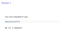 |
|
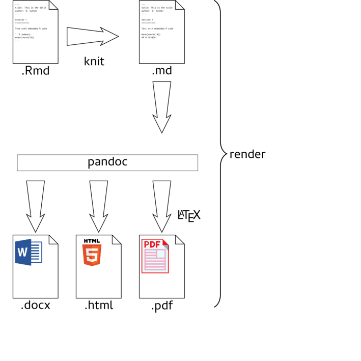
In order to make most use of Rmarkdown, it is important to have a basic understanding that it is not
a single tool, but rather a series of tools (including the knit function within the
knitr R package and the external command line universal document conversion tool called pandoc).
Rstudio
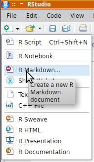
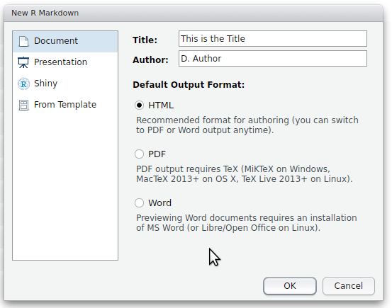
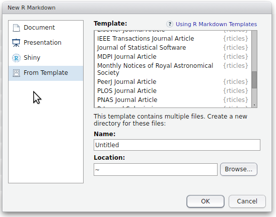
The rmarkdown package is built into more recent versions of Rstudio. To begin creating an Rmarkdown document, simply:
- go to the File menu and select 'Rmarkdown'
- provide a title and author
- select one of the three document types (note, these can be easily changed at any time).
Note, in order to compile the markdown into a pdf, you will need one of the flavours of LaTeX to be installed on your machine. LaTeX is an mature, open source document preparation system.
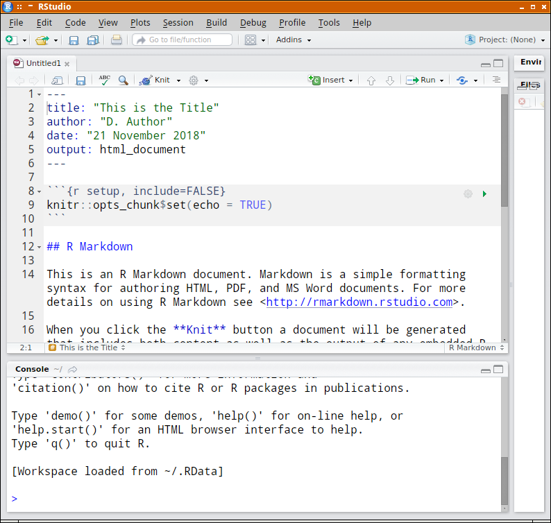
A starting Rmarkdown document is created for you. Notice the following:
- initially the document is unamed and unsaved. Before you can render this to another format, you will need to make sure it is saved.
- a YAML meta data header has been added to the top of the new document. Rather than hide all the settings associated with a document within a bunch of menus, most of the settings can be defined in this directly editable meta data header. Since we nominated a HTML document, the output is specified to be HTML. To specify a different format, simply alter the text.
- R code chunks are defined between a pair of three backticks (```) and with the default appearance theme, have a grey background.
- the toolbar has a new icon that looks like a ball of wool and knitting needles (it looks like that because that is what it is!). Clicking on this icon will start the rendering process (starting with a prompt for a path and filename.
- clicking on the down arrow to the right of the ball of wool icon allows the format of the rendered document to be altered.
- clicking on the cog icon to the right of the ball of wool icon and selecting 'Output options' brings up a dialog box that allows further alterations to the looks and style of the output document.
For the remainder of this tutorial, we will use the Rmardown document and render() pathway as it will work across all editors and plain R itself. Needless to say, the code illustrated will work the same in Rstudio, yet without the need to run the render() function - that is taken care of by the ball of wool icon.
Markdown elements
Tutorial 17.3 introduced the markdown language. Some of that information will be repeated here, yet you are invited to consult Tutorial 17.3 for more information.
Text formatting
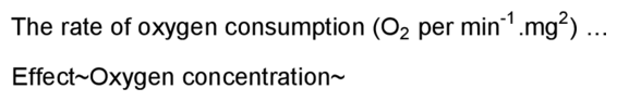
Simple super and subscript
| Markdown |
|---|
The rate of oxygen consumption (O~2~ per min^-1^.mg^2^) ... Effect~Oxygen\ concentration~ |
Result |
 |
Section headings
| Markdown | |
|---|---|
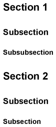
Section 1 =========== Subsection ------------ ### Subsubsection # Section 2 ## Subsection ### Subsection |
Note, there are two ways to define section headings:
|
Result |
 |
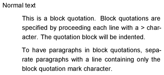
Block quotations
| Markdown |
|---|
Normal text > This is a block quotation. Block quotations are specified by > proceeding each line with a > character. The quotation block > will be indented. > > To have paragraphs in block quotations, separate paragraphs > with a line containing only the block quotation mark character. |
Result |
 |
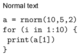
Verbatim blocks
| Markdown |
|---|
Normal text

~~~~
a = rnorm(10,5,2)
for (i in 1:10) {
  print(a[1])
}
~~~~
|
Result |
 |
Lists
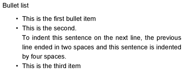
Bullet lists
| Markdown |
|---|
Bullet list

* This is the first bullet item
* This is the second.
  To indent this sentence on the next line,
    the previous line ended in two spaces and
    this sentence is indented by four spaces.
* This is the third item
|
Result |
 |
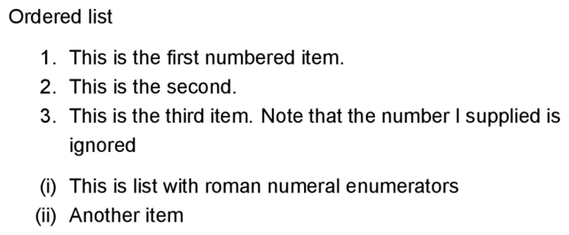
Ordered lists
| Markdown |
|---|
Ordered list 1. This is the first numbered item. 2. This is the second. 1. This is the third item. Note that the number I supplied is ignored (i) This is list with roman numeral enumerators (ii) Another item |
Result |
 |
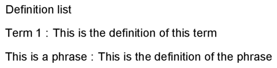
Definition lists
| Markdown |
|---|
Definition list

Term 1
    :  This is the definition of this term

This is a phrase
    :  This is the definition of the phrase
|
Result |
 |
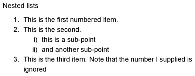
Nested lists
| Markdown |
|---|
Nested lists 1. This is the first numbered item. 2. This is the second. i) this is a sub-point ii) and another sub-point 1. This is the third item. Note that the number I supplied is ignored |
Result |
 |
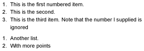
List ends
| Markdown |
|---|
1. This is the first numbered item. 2. This is the second. 1. This is the third item. Note that the number I supplied is ignored 1. Another list. 2. With more points |
Result |
 |
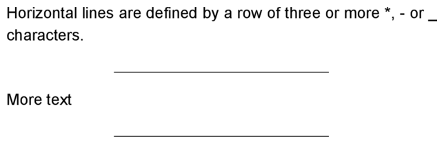
Horizontal lines
| Markdown |
|---|
Horizontal lines are defined by a row of three or more *, - or _ characters. *** More text -------- |
Result |
 |
Math and equations
| Markdown |
|---|
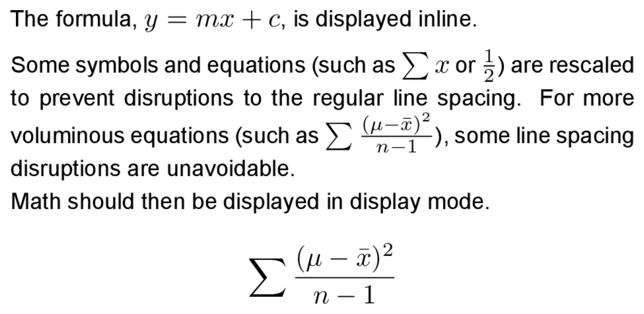
The formula, $y=mx+c$, is displayed inline.

Some symbols and equations (such as
$\sum{x}$ or $\frac{1}{2}$) are rescaled
to prevent disruptions to the regular
line spacing.
For more voluminous equations (such as
$\sum{\frac{(\mu - \bar{x})^2}{n-1}}$),
some line spacing disruptions are unavoidable.
Math should then be displayed in display mode.
$$\sum{\frac{(\mu - \bar{x})^2}{n-1}}$$
|
Result |
 |
Referencing
Internal links
| Markdown |
|---|
# Introduction {#sec:Intro}
Bla Bla Bla [cap]: #cap

# Section 2
See the [introduction](#sec:Intro) and in particular [cap].
|
Result |
 |
External links
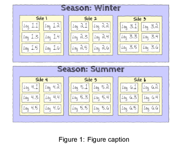
Images
| Markdown |
|---|
 |
Result |
 |
Footnotes
| Markdown |
|---|
To create a footnote[^note1] [^note1]: A footnote marker cannot contain any spaces. |
Result |
 |
Code chunks
Reproducible research is a data analyses concept that promotes publishing of all analysis source, outcomes and supporting commentary (such as a description of methodologies and interpretation of results) in such a way that others can reproduce the findings for verification. Ideally, this works best when the documentation and source codes are woven together into a single document. Traditionally, this would involve substantial quantities of 'cutting and pasting' from statistical software into document authoring tools such as LaTeX, html or Microsoft Word. Of course, any minor changes in the analyses then would necessitate replacements of the code in the document as well as replacing any affected figures or tables. Keeping everything synchronized was a bit of a battle.
This is where packages like knitr come in. Knitr evaluates blocks of code within a document and converting both the code and output into the same format as the surrounding document (e.g. LaTeX or html). This scheme greatly facilitates reproducible research by allowing the document and all source code to be contained in a single file or related files.
Code chunks are defined as starting with the sequence ```{ and end with ```. For example, to define a simple R code chunk, we would include:
```{r name}
```
Any code that appears in the lines between the opening and closing chunk sequences will be
evaluated by R.
Importantly, to evaluate the code chunks embedded within an Rmarkdown document, the code is passed through a new R session. This means that although you might be testing the code in an R console (or Rstudio) as you write the code, it is important that the code be completely self contained. Therefore, if the code relies on a package or external function, these must be loaded as part of the script.
As a minimum, it is advisable that each chunk be given a unique name (name in the example below). There are numerous additional arguments (options) that can be included in the chunk header. These control the behaviour of the knitting process and the common ones are listed in the following table.
| Option | Description | LaTeX | HTML |
|---|---|---|---|
| Text output | |||
| echo | either:
|
Yes | Yes |
| eval | either:
|
Yes | Yes |
| results | either:
|
Yes | Yes |
| warning | either:
|
Yes | Yes |
| error | either:
|
Yes | Yes |
| message | either:
|
Yes | Yes |
| cache |
|
Yes | Yes |
| dependson |
|
Yes | Yes |
| Code decoration | |||
| tidy | either:
|
Yes | Yes |
| tidy.opts | a list of options passed on to the tidying function. For example, tidy.opts = list(width.cutoff = 60) restricts the width of R output to 60 characters wide. | Yes | Yes |
| prompt | TRUE or FALSE (whether to include R prompts in the echoed code) | Yes | Yes |
| comment | the comment character used before output (defaults to ##) | Yes | Yes |
| highlight | TRUE or FALSE (whether to apply syntax highlighting to the code) | Yes | Yes |
| size | the font size for code and output | Yes | No |
| background | the color of the code and output background | Yes | No |
| Text output | |||
| results | either:
|
Yes | Yes |
| Figures | |||
| fig.width | Width (in inches) of the stand-alone figure | Yes | Yes |
| fig.height | Height (in inches) of the stand-alone figure | Yes | Yes |
| out.width | Width (in inches) of the figure in the output document | Yes | Yes |
| out.height | Height (in inches) of the figure in the output document | Yes | Yes |
| fig.cap | The figure caption associated with the figure | Yes | Yes |
| fig.align | Alignment of the figure on the page - one of left, right or center | Yes | Yes |
Kitting tables
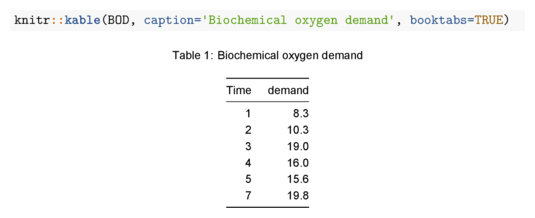
Tables deserve special treatment hear. There are numerous routines (and packages) to support the elegant production of tables from R. I will illustrate arguably the simplest (kable). The kable function is part of the knitr package and can be extended using the kableExtra package. To illustrate, we will use the built in dataset called cars).
| *.Rmd |
|---|
  ```{r BODData}
  knitr::kable(BOD, caption="Biochemical oxygen demand", booktabs=TRUE)
  ```
|
Output |
 |
Citations (bibliography)
It is always important to cite the original source of an idea or finding, and an analysis document is +\n o exception. It is often and the statistical development stage that methodological references are consulted. It is vital that any used sources are documented - particularly before they are misplaced or forgotten.
In text citations and the associated references section are supported via the bibtex format in rmarkdown. The bibtex format is one of the major formats provided for export by journals and databases like citeulike and crossref.
A bitex database is a plain text file with specific tag pairs to define the different components (fields) of a reference. To illustrate lets generate a bibtex database with two references.
  @article{Bolker-2008-127,
  author = {Bolker, B. M. and Brooks, M. E. and Clark, C. J. and Geange, S. W. and Poulsen,
  J. R. and Stevens, H. H. and White, J. S.},
  journal = {Trends in Ecology and Evolution},
  number = {3},
  pages = {127-135},
  title = {Generalized linear mixed models: a practical guide for ecology and evolution},
  volume = {24},
  year = {2008}
  }

  @book{goossens93,
  author    = "Michel Goossens and Frank Mittlebach and Alexander Samarin",
  title     = "The LaTeX Companion",
  year      = "1993",
  publisher = "Addison-Wesley",
  address   = "Reading, Massachusetts"
  }
For more information on the different reference types and fields, refer to Tutorial 17.1.
If you are using Rstudio and have the citr package loaded, then, if you select 'Insert citations' from the the 'Addins' toolbar icon, you will be able to search your bibtex bibliography and selected references will be added to your document.
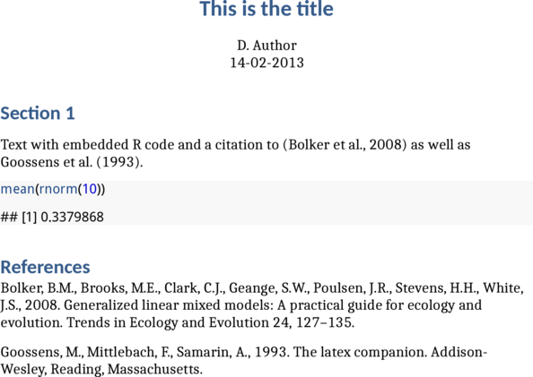
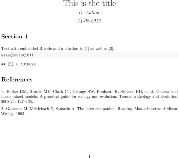
In addition to the bibtex file, we typically want to be able to specify the format of the bibliography and in-text citations. By default, the Chicago author-date format is applied. However, by supplying a CSL 1.0 style file, the format can be altered to suit any journal or style. Here is a repository of CSL 1.0 styles. Simply search for the one(s) you want and download them. We will try both the marine-pollution-bulletin.csl and plos-biology.csl styles as examples.
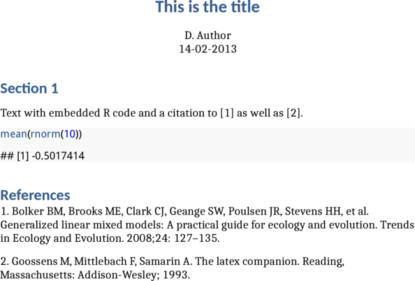
Create the above code (or cut and paste into your editor) and save it as refs.bib (or some other name ending in .bib) and then modify the YAML header to specify this bibliography.
---
title: This is the title
author: D. Author
date: 14-02-2013
bibliography: refs.bib
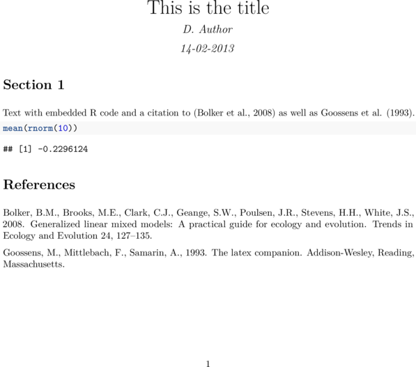
csl: marine-pollution-bulletin.csl
...
# Section 1
Text with embedded R code and a citation to [@Bolker-2008-127] as well as @goossens93.
```{r Summary}
mean(rnorm(10))
```
References
============
Create the above code (or cut and paste into your editor) and save it as refs.bib (or some other name ending in .bib) and then modify the YAML header to specify this bibliography.
  ---
  title: This is the title
  author: D. Author
  date: 14-02-2013
  bibliography: refs.bib
  csl: plos-biology.csl
  ...

  # Section 1
  Text with embedded R code and a citation to [@Bolker-2008-127] as well as @goossens93.

  ```{r Summary}
  mean(rnorm(10))
  ```

  References
  ============
Changing the look
Recall from Tutorial 17.3 that the meta data of a markdown file is defined in a special YAML block (which is normally, yet not necessarily, positioned at the top of the markdown file). In the example above, this was used to define the title, an author, date and bibliography and can also be used to specify the broad type of output (PDF, HTML, Word). The YAML block is also used to determine the style and formatting of the output. In this section, we will explore some of the major customizations available from small changes to the YAML block.
The following table lists the main simple customizations that can be applied and which document type they can be applied to. In the table (yes/no) are the same as (true/false). Values in square braces are alternatives to the default values. I have purposely used settings (in the Options column) that contrast the default settings so that the effects are very obvious. They do not constitute any form of recommendation.
| Option | Description | HTML | Word | |
|---|---|---|---|---|
| toc: yes | Include a table of contents (default: no) | ✔ | ✔ | ✔ |
| toc_depth: 2 | Depth of the table of contents (default: 3) | ✔ | ✔ | ✔ |
| number_sections: yes | Number the sections (default: no) | ✔ | ✔ | ✖ |
| fig_width: 5 | Width of figures in inches (default: 6) | ✔ | ✔ | ✔ |
| fig_height: 5 | Height of figures in inches (default: 4.5) | ✔ | ✔ | ✔ |
| df_print: kable | Processing of data.frames (default: default) [kable,tibble,paged] | ✔ | ✔ | ✔ |
| highlight: zenburn | R code syntax highlighting (default: default) [tango, pygments, kate, monochrome, espresso, zenburn, haddock, textmate] | ✔ | ✔ | ✔ |
| code_folding: hide | Hide/reveal code blocks in output (default: none) [show,hide] | ✖ | ✔ | ✖ |
| theme: spacelab | A pre-packaged page theme (default: default) [cerulean, journal, flatly, readable, spacelab, united, cosmo, lumen, paper, sandstone, simplex, yeti] | ✖ | ✔ | ✖ |
| latex_engine: xelatex | The LaTeX engine to use (default: pdflatex) [xelatex, lualatex] | ✔ | ✖ | ✖ |
Lets now explore what the effect of the above customizations have on the output format of a very simple rmarkdown document..
| Markdown |
|---|
---
title: This is the title
author: D. Author
date: 14-02-2013
output:
pdf_document:
toc: yes
toc_depth: 2
number_sections: yes
fig_width: 5
fig_height: 5
df_print: kable
highlight: zenburn
...
# Section 1
Text with embedded R code.
```{r Summary}
mean(rnorm(10))
```
```{r head}
head(cars)
```
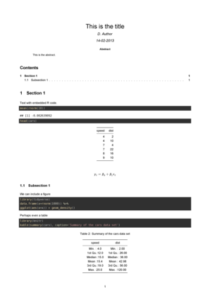
## Subsection 1
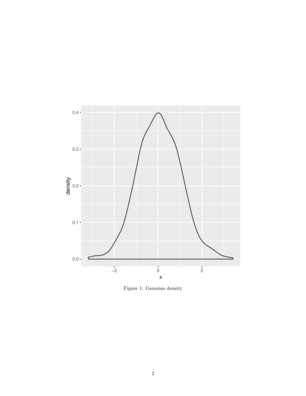
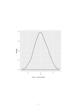
We can include a figure
```{r Plot, fig.cap='Gaussian density.',message=FALSE}
library(4.5idyverse)
data.frame(x=rnorm(1000)) %$gt;%
ggplot(aes(x=x)) + geom_density()
```
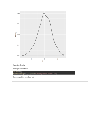
Perhaps even a table
```{r table}
library(knitr)
kable(summary(cars), caption='Summary of the cars data set')
```
|
PDF result |
library(rmarkdown) render('min.Rmd') 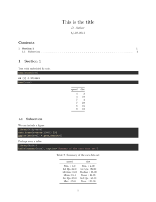
 |
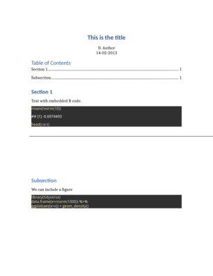
| Markdown |
|---|
---
title: This is the title
author: D. Author
date: 14-02-2013
output:
  html_document:
    toc: yes
    toc_depth: 2
    number_sections: yes
    fig_width: 5
    fig_height: 5
    df_print: kable
    highlight: zenburn
    code_folding: hide
    theme: spacelab
...

# Section 1
Text with embedded R code.

```{r Summary}
mean(rnorm(10))
```
```{r head}
head(cars)
```

## Subsection
We can include a figure

```{r Plot, fig.cap='Gaussian density.',message=FALSE}
library(tidyverse)
data.frame(x=rnorm(1000)) %$gt;%
ggplot(aes(x=x)) + geom_density()
```
Perhaps even a table

```{r table}
library(knitr)
kable(summary(cars), caption='Summary of the cars data set')
```
|
HTML result |
| Markdown |
|---|
---
title: This is the title
author: D. Author
date: 14-02-2013
output:
  word_document:
    toc: yes
    toc_depth: 2
    fig_width: 5
    fig_height: 5
    df_print: kable
    highlight: zenburn
...

# Section 1
Text with embedded R code.

```{r Summary}
mean(rnorm(10))
```
```{r head}
head(cars)
```

## Section 1

We can include a figure

```{r Plot, fig.cap='Gaussian density.',message=FALSE}
library(tidyverse)
data.frame(x=rnorm(1000)) %>%
ggplot(aes(x=x)) + geom_density()
```
Perhaps even a table

```{r table}
library(knitr)
kable(summary(cars), caption='Summary of the cars data set')
```
|
Word result (well - approximately) |
 |
It is possible to include multiple output statements in the YAML block, thereby defining the basic processing options for multiple output formats. For example, to specify the above setting for each of PDF, HTML and Word output formats the YAML block might look like:
  ---
  title: This is the title
  author: D. Author
  date: 14-02-2013
  output:
    pdf_document:
      toc: yes
      toc_depth: 2
      number_sections: yes
      fig_width: 5
      fig_height: 5
      df_print: kable
      highlight: zenburn
    html_document:
      toc: yes
      toc_depth: 2
      number_sections: yes
      fig_width: 5
      fig_height: 5
      df_print: kable
      highlight: zenburn
      code_folding: hide
      theme: spacelab
    word_document:
      toc: yes
      toc_depth: 2
      fig_width: 5
      fig_height: 5
      df_print: kable
      highlight: zenburn
  ...
If we were to render an rmarkdown document with the above YAML block via the render()
function (and without providing the output_format argument),
the underlying engine will attempt to generate a PDF file (since the pdf_document is the
first one defined in the YAML block). However, if we do specify a different output_format argument,
the associated customizations will be applied when rendering the document. The customizations can
be different for each of the document types (PDF, HTML and Word).
In addition to the above settings that can be applied to different output formats and yet are specified as third-level arguments (that is under each document type), there are also settings that can be applied to multiple output document formats yet that are applied as top-level arguments. These are listed in the following table and example outputs.
| Option | Description |
|---|---|
| fontsize: 10pt | Document font size [10pt, 11pt, 12pt] |
| abstract: This is the abstract... | An abstract |
Although rmarkdown (along with knitr and pandoc) is the Swiss Army knife of document preparation -- in that the same source document can be used to produce multiple output formats -- each of these three formats provide different utilities. As such, it is often desirable to customize the outputs to make best use of different formats.
- PDF documents provide a good way to communicate research in a a controlled and universal manner. In this render workflow, PDF documents are created via LaTeX. Styling in LaTeX is controlled via macros defined in the document preamble. Hence, major customizations are brought about by dictating changes to the preamble.
- HTML documents provide the presentation of dynamic content. Styling in HTML documents is largely controlled via style sheets and/or scripts (particularly javascript).
- Word documents provide a document format that is accessable to non-scientists. Styling in Word is provided by the element styles defined in the document itself - which are often imposed by a template.
Since styling is each of these formats is quite different and as some of these customizations can get extensive, we will treat each document type separately in the following sections.
PDF documents
The styling information in LaTeX is defined in the document preamble. A markdown LaTeX template is essentially a skeleton LaTeX document with an extensive collection of conditional statements that allow the preamble to be customized based on the options indicated in the markdown YAML header.
In Tutorial 17.1, we briefly introduced the structure of a LaTeX document. Importantly, the preable of the LaTeX document defines a document class followed by a series of macros (similar to constants and functions in other languages) that define the settings and styling of the document.
When pandoc converts a markdown document into a LaTeX document, it accesses a template which is used to generate the preable for the LaTeX document. The template system is designed so that information specified in the YAML block of the markdown document can be used to govern certain aspects of the resulting LaTeX preamble
The following table, lists some of the customizations that can be included as top-level (not indented) YAML meta data for PDF output. Note, these can be present when rendering to other formats, they will just be ignored.
| Option | Description |
|---|---|
| fontsize: 11pt | The size of the base font (default: 12pt) |
| documentclass: book | LaTeX document class (default: article, minimal) [book] |
| classoption: a4paper | Options for documentclass [oneside,a4paper] |
| geometry: margin=1cm | Options for the geometry class |
| fontsize: 11pt | Document font size |
| fontfamily: mathpazo | Document fonts (only available when using pdflatex) |
| mainfont: Arial | Document fonts (only available when using xelatex) |
| sansfont: Arial | Document fonts (only available when using xelatex) |
| monofont: Courier | Document fonts (only available when using xelatex) |
| mathfont: mathpazo | Document fonts (only available when using xelatex) |
| linkcolor: blue | Color of internal links |
| urlcolor: blue | Color of external links |
| citecolor: blue | Color of citation links |
fc-list --format="%{family[0]}\n" | sort | uniq
Alternatively, within R:
library(sysfonts)
unique(font_files()$family)
  [1] "Cabin"                      "Cantarell"                  "EB Garamond 08"
  [4] "EB Garamond 12"             "EB Garamond Initials Fill1" "EB Garamond Initials Fill2"
  [7] "EB Garamond Initials"       "FontAwesome"                "FreeMono"
 [10] "FreeSans"                   "FreeSerif"                  "Linux Biolinum Keyboard O"
 [13] "Linux Biolinum O"           "Linux Libertine Display O"  "Linux Libertine Initials O"
 [16] "Linux Libertine Mono O"     "Linux Libertine O"          "Lobster Two"
 [19] "STIXGeneral"                "STIXIntegralsD"             "STIXIntegralsSm"
 [22] "STIXIntegralsUp"            "STIXIntegralsUpD"           "STIXIntegralsUpSm"
 [25] "STIXNonUnicode"             "STIXSizeFiveSym"            "STIXSizeFourSym"
 [28] "STIXSizeOneSym"             "STIXSizeThreeSym"           "STIXSizeTwoSym"
 [31] "STIXVariants"               "STIX"                       "STIX Math"
 [34] "Accanthis ADF Std"          "Accanthis ADF Std No2"      "Accanthis ADF Std No3"
 [37] "Gillius ADF"                "Gillius ADF Cd"             "Gillius ADF No2"
 [40] "Gillius ADF No2 Cd"         "Universalis ADF Cd Std"     "Universalis ADF Std"
 [43] "GFS Artemisia"              "Asana Math"                 "Comfortaa"
 [46] "GFS Complutum"              "Caladea"                    "Carlito"
 [49] "DejaVu Sans"                "DejaVu Sans Condensed"      "DejaVu Sans Light"
 [52] "DejaVu Sans Mono"           "DejaVu Serif"               "DejaVu Serif Condensed"
 [55] "GFS Didot"                  "GFS Didot Rg"               "Droid Arabic Kufi"
 [58] "Droid Arabic Naskh"         "Droid Naskh Shift Alt"      "Droid Sans Arabic"
 [61] "Droid Sans Armenian"        "Droid Sans"                 "Droid Sans Ethiopic"
 [64] "Droid Sans Fallback"        "Droid Sans Georgian"        "Droid Sans Hebrew"
 [67] "Droid Sans Japanese"        "Droid Sans Mono"            "Droid Serif"
 [70] "EB Garamond 08 SC"          "Gentium Basic"              "Gentium Book Basic"
 [73] "GentiumAlt"                 "Gentium"                    "Inconsolata"
 [76] "Junicode"                   "Lato Black"                 "Lato"
 [79] "Lato Hairline"              "Lato Heavy"                 "Lato Light"
 [82] "Lato Medium"                "Lato Semibold"              "Lato Thin"
 [85] "Liberation Mono"            "Liberation Sans"            "Liberation Sans Narrow"
 [88] "Liberation Serif"           "cmex10"                     "cmmi10"
 [91] "cmr10"                      "cmsy10"                     "esint10"
 [94] "eufm10"                     "msam10"                     "msbm10"
 [97] "rsfs10"                     "stmary10"                   "wasy10"
[100] "Andale Mono"                "Arial"                      "Arial Black"
[103] "Comic Sans MS"              "Courier New"                "Georgia"
[106] "Impact"                     "Times New Roman"            "Trebuchet MS"
[109] "Verdana"                    "Webdings"                   "GFS Neohellenic Rg"
[112] "GFS Olga"                   "OpenSymbol"                 "GFS Solomos"
  ---
  title: This is the title
  author: D. Author
  date: 14-02-2013
  output:
    pdf_document:
      toc: yes
      toc_depth: 2
      number_sections: yes
      fig_width: 5
      fig_height: 5
      df_print: kable
      highlight: zenburn
      latex_engine: xelatex
  fontsize: 10pt
  geometry: margin=1cm
  mainfont: Arial
  mathfont: LiberationMono
  monofont: DejaVu Sans Mono
  classoption: a4paper
  abstract: This is the abstract.
  urlcolor: red
  ...

  # Section 1
  Text with embedded R code.

  ```{r Summary}
  mean(rnorm(10))
  ```
  ```{r head}
  head(cars)
  ```

  $$
  y_i = \beta_0 + \beta_1 x_i
  $$

  ## Subsection 1

  We can include a figure

  ```{r Plot, fig.cap='Gaussian density.',message=FALSE}
  library(4.5idyverse)
  data.frame(x=rnorm(1000)) %$gt;%
  ggplot(aes(x=x)) + geom_density()
  ```

  Perhaps even a table

  ```{r table}
  library(knitr)
  kable(summary(cars), caption='Summary of the cars data set')
  ```
Templates
More wholesale style changes are supported by the use of templates. Whilst pandoc comes with a default LaTeX template, it is possible to create your own so as to provide even greater control over the output style. To illustrate, we will create a very minimal template (lets call it latex.template).
| latex.template | min.Rmd |
|---|---|
  \documentclass{$documentclass$}
  \usepackage{hyperref}
  \begin{document}
  $body$
  \end{document}
|
---
output:
  pdf_document:
    template: latex.template
    highlight: null
documentclass: article
...

Section
===========
Text with embedded R code.

```{r head}
head(cars)
```

$$
y_i = \\beta_0 + \\beta_1 x_i
$$
|
render('simple.Rmd')

In this way, it is possible to construct a complete template so as to have full control over the output document style.
Packaged templates
The rticles package provides additional Rmarkdown pandoc templates as well as wrapper functions to
help put all the template and associated files in the correct location. Furthermore, if the rticles package
is installed, then Rstudio will have additional templates available from the new R markdown dialog box.
The same can be completed in script using the draft function from the rmarkdown package.
rmarkdown::draft(file='plos.Rmd', template='plos_article', package='rticles', edit=FALSE)
rmarkdown::render(file='plos/plos.Rmd')

rmarkdown::draft(file='pnas.Rmd', template='pnas_article', package='rticles', edit=FALSE)
rmarkdown::render(file='pnas/pnas.Rmd')

rmarkdown::draft(file='elsevier.Rmd', template='elsevier_article', package='rticles', edit=FALSE)
rmarkdown::render(file='elsevier/elsevier.Rmd')


HTML
Unlike PDF and Word documents, HTML documents have the potential to be more interactive and dynamic. This allows the presentation of content to be more flexible. Consequently, there are numerous customizations that can be applied to HTML documents that cannot be applied to other document types.
There are a number of additional second-level YAML arguments that can be used to customize HTML documents - these are listed in the following table.
| Option | Description |
|---|---|
| toc_float: yes | Float the table of contents in a panel on the left side of the document. Other options are also available (see below). |
| collapse: yes | Collapse table of contents to just first level headings |
| smooth_scroll: yes | Animate page scrolling when items selected from table of contents. |
| self_contained: yes | Whether to generate self contained HTML (other than Mathjax). |
Tabbed sections
One way to maintain present content in a compact manner without excluding material is to have content that is hidden until it it revealed. This behaviour is supported via tabsets. Tabsets are defined by placing a .tabset class attribute. All subheadings under this heading will then be rendered as tabs.
---
title: This is the title
author: D. Author
date: 14-02-2013
output:
  html_document:
    toc: yes
    toc_depth: 2
    number_sections: yes
    fig_width: 5
    fig_height: 5
    df_print: kable
    highlight: zenburn
    code_folding: hide
    theme: spacelab
    toc_float: yes
    collapse: no
...

# Section 1
Text with embedded R code.

```{r Summary}
mean(rnorm(10))
```
```{r head}
head(cars)
```

## Output {.tabset .tabset-fade}

### Figure
We can include a figure

```{r Plot, fig.cap='Gaussian density.',message=FALSE}
library(tidyverse)
data.frame(x=rnorm(1000)) %>%
ggplot(aes(x=x)) + geom_density()
```

### Table

```{r table}
library(knitr)
kable(summary(cars), caption='Summary of the cars data set')
```
Style sheets
The general look and style of a HTML document is controlled via Cascading Style Sheet (CSS). A CSS comprises one or more files that define the styling of the HTML elements. Rmarkdown has a default HTML template and style sheet that are used by pandoc when converting markdown documents to HTML documents. It is possible to provide alternate templates and CSS.
For example, to nominate an additional CSS that will be applied to the default template after the default CSS file, we can use the css: second-level argument. Since, this additional CSS is applied after the default CSS, any styles defined within the additional CSS will take precedence.
For a simple example, if we wanted all the Section headings to be a light blue color and the title to be the same color blue colour as the dropdown menu background, we could define the following:
| style.css | doc.Rmd |
|---|---|
  h1, h2, h3 {
    color: lightblue;
  }
  h1.title {
    color: #446e9b;
  }
|
---
title: This is the title
author: D. Author
date: 14-02-2013
output:
  html_document:
    toc: yes
    toc_depth: 2
    number_sections: yes
    fig_width: 5
    fig_height: 5
    df_print: kable
    highlight: zenburn
    code_folding: hide
    theme: spacelab
    toc_float: yes
    collapse: no
    css: styles.css
...

# Section 1
Text with embedded R code.

```{r Summary}
mean(rnorm(10))
```
```{r head}
head(cars)
```

## Output {.tabset .tabset-fade}

### Figure
We can include a figure

```{r Plot, fig.cap='Gaussian density.',message=FALSE}
library(tidyverse)
data.frame(x=rnorm(1000)) %>%
ggplot(aes(x=x)) + geom_density()
```

### Table

```{r table}
library(knitr)
kable(summary(cars), caption='Summary of the cars data set')
```
|