Worksheet 10 - Generalized Linear Mixed effects Models (GLMM's)
23 April 2011
Model diagnostics in mixed linear models
Obtaining glmmADMB
Collections of datasets
BB glmm talk
Another collection of datasets - mainly for simpler stats
A couple of mixed model examples with R script
Knitr tutorial
GGplot2 tutorial
BB comparative glmm rnw
Comparative owls BB
News thread on zero-inflation priors
Comparative glmm
JH course notes on MCMCglmm
visualizing Bayes theorem
Good MCMC explanation for social scientists Really good lecture overview
http://carrot.mcb.uconn.edu/~olgazh/bioinf2010/class31.html - has stuff about normalizing constant http://sites.stat.psu.edu/~mharan/MCMCtut/MCMC.html - some R simulations etc, explainations https://docs.google.com/a/monash.edu/viewer?a=v&q=cache:k0vQ79b1D6cJ:seis.bris.ac.uk/~frwjb/materials/ver2mcmc.pdf+posterior+distribution+MCMC&hl=en&gl=au&pid=bl&srcid=ADGEESievALjj3OtlGI1RyEXtZ1P_wFgtzMbNrKC9fs3nCTwJ5oidsJS-JAs1Q4G2QXazFYu_-wXQDi4XHHeQQvQNvDbrROg7MrA_vMSueovzWZgH58xsVz0unaqGFkB1YywpF8zxGOV&sig=AHIEtbSVtI0a3lf_UWCNXjybamzDbzrsdQ - simple explanation of MCMC https://docs.google.com/a/monash.edu/viewer?a=v&q=cache:ER08bstYWdwJ:www.statistics.du.se/essays/D12_SunLei.pdf+MCMC+MME+solutions&hl=en&gl=au&pid=bl&srcid=ADGEEShOkzNWKamWhOx0sHiBzImMY_1pOxgJe3Y7opzMnrmpy4NbBgkjmhrFJKusXyPHLrFBJApLdXeyl7e66_UXdqw8q1hc9ixADnyDV9DYFYV2Ff146CQsanRt6xx-Ent6SNPhmqM8&sig=AHIEtbRTqi8rxE6vSEnLn1MFrhYy4Yk5-w
ℒ
As a dataset becomes more complex (due to design and other statistical issues), the number of ways that the data can be analysed increases. It is true that some methods will be more valid than others under certain circumstances, however each technique has its pros and cons. And there is generally no "best" solution. It is therefore strongly suggested that more complex analyses be performed with a range of techniques and the outcomes compared. If there is general consensus, then any one of the techniques are appropriate and thus the simplest approach is perhaps justified. If there is not consensus, then the techniques and outcomes should be evaluated in light of the pros and cons on the technique. Although it is likely that each technique will have sort comings, provided you are aware of these and can justify your selection on the basis of minimized impacts of these sort comings, others should respect your choices.
For each of the examples below, we will proceed to analyse them via numerous techniques. In part this should demonstrate the use of these various techniques. Yet it should also highlight the importance of using a variety of techniques and evaluating their suitability's on a case by case basis.
Nested ANOVA - one between factor
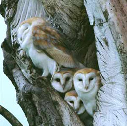
Zuur et al (2009) used a dataset of Roulin and Bersier (2007) on which the begging behaviour of barn owl nestlings to illustrate various mixed effects concepts. Barn owl nestlings had previously been shown to engage in 'negotiations' in which they communicate their relative levels of hunger to each other. Apparently, they pre-compete via calling frequency prior to the return of the parent as a partial alternative to more costly direct competitive begging for food from the parent.
To further explore this behaviour, Roulin and Bersier (2007) recorded (amongst other responses), the number of nestling calls in the 30 period prior to the return of the adult from each of 27 nests on two consecutive nights. On the first night, half the nests were provided with additional prey (satiated food treatment), while the other half had any food not immediately consumed by nestlings removed (deprived food treatment). These treatments were hence reversed on the second night.
In addition to the food treatment manipulation, the researchers recorded the sex of the parent returning with the food and the size of the brood (as the number of nestling calls is likely to increase with increasing numbers of siblings).
Download Owls data set
| Format of owls.csv data files | |||||||||||||||||||||||||||||||||||||||||||||||||||||||
|---|---|---|---|---|---|---|---|---|---|---|---|---|---|---|---|---|---|---|---|---|---|---|---|---|---|---|---|---|---|---|---|---|---|---|---|---|---|---|---|---|---|---|---|---|---|---|---|---|---|---|---|---|---|---|---|
|
 |
||||||||||||||||||||||||||||||||||||||||||||||||||||||
> #download.file('http://www.highstat.com/Book2/ZuurDataMixedModelling.zip',
> #               destfile='tmp.zip')
> #unzip('tmp.zip',files='Owls.txt')
> #Owls <- read.table('Owls.txt',header=TRUE)
> #head(Owls)
> #write.table(Owls,'../downloads/data/owls.csv', quote=F, row.names=F,
> #   sep=',')
> owls <- read.table("../downloads/data/owls.csv", header = TRUE, sep = ",",
+     strip.white = TRUE)
> head(owls)
        Nest FoodTreatment SexParent ArrivalTime SiblingNegotiation BroodSize NegPerChick
1 AutavauxTV      Deprived      Male       22.25                  4         5         0.8
2 AutavauxTV      Satiated      Male       22.38                  0         5         0.0
3 AutavauxTV      Deprived      Male       22.53                  2         5         0.4
4 AutavauxTV      Deprived      Male       22.56                  2         5         0.4
5 AutavauxTV      Deprived      Male       22.61                  2         5         0.4
6 AutavauxTV      Deprived      Male       22.65                  2         5         0.4
Before leaping in to any analyses, as usual we will begin by exploring the data.
- Boxplots of SiblingNegotiations per Food treatment and parent sex combination.
> library(ggplot2)
> ggplot(data = owls) + geom_boxplot(aes(y = SiblingNegotiation, x = Nest)) +
+     facet_grid(SexParent ~ FoodTreatment)
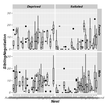
As is often the case for count data, there is evidence of non-normality and non-homogeneity of variance. Furthermore, there are many zeros. We could attempt to address the former issues by normalizing the response variable by applying a square-root (or forth root) transformation. Alternatively, rather than try to make these data conform to a Gaussian distribution, we could instead model the data against a more suitable distribution (such as a Poisson distribution).
- Scatterplots of SiblingNegotiations against brood size for each food treatment and parent sex combination.
> library(ggplot2)
> ggplot(data = owls) + geom_point(aes(y = SiblingNegotiation, x = BroodSize)) +
+     geom_smooth(aes(y = SiblingNegotiation, x = BroodSize), method = "lm") +
+     facet_grid(SexParent ~ FoodTreatment)
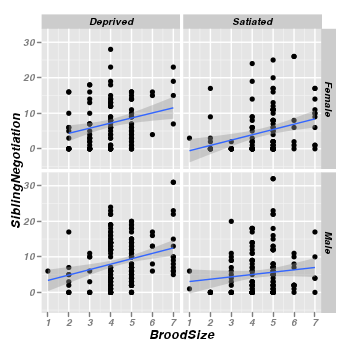
The relationship between sibling negotiations and brood size is confirmed. Furthermore, there is no real suggestion that the nature of this relationship differs substantially between different treatment (food and parent sex) combinations. Hence, brood size would seem a potentially useful and suitable covariate.
-
Count the number of replicates in each treatment combination and thus design balance.\
Clearly, the design is not balanced.
> replications(~FoodTreatment * SexParent, data = owls)$FoodTreatment FoodTreatment Deprived Satiated 320 279 $SexParent SexParent Female Male 245 354 $`FoodTreatment:SexParent` SexParent FoodTreatment Female Male Deprived 123 197 Satiated 122 157> #is the design balanced? > !is.list(replications(~FoodTreatment * SexParent, data = owls))
[1] FALSE
We are now in a position to start analysing these data. The design is almost a classic randomized block or repeated measures, albeit very unbalanced. Nests are the plots or blocks that are each measured on multiple occasions. The food treatment was manipulated such that each nest received both levels of the treatment. Hence food treatment is a within block (nest) treatment. Although the sex of the returning parent was not under the control of the researchers, each nest nevertheless was visited by both parents and thus parent sex is also a within nest effect.
Via lmer (linear mixed effects)
> library(lme4)
-
Lets begin by analysing these data as a regular linear mixed effects model. After all, if the
non-normality and non-homogeneity of variance issues do not manifest analytically, then the more
simplistic approach is preferred.
> library(lme4)
> owls.lmer <- lmer(SiblingNegotiation ~ FoodTreatment * SexParent +
+     BroodSize + (1 | Nest), family = gaussian, data = owls)
-
Examine the residuals
There is evidence of non-homogeneity of variance
> plot(residuals(owls.lmer) ~ fitted(owls.lmer))

-
Examine the QQ normal plot to see whether the non-homogeneity of variance could be the result of non-normality.
Whilst there is no evidence of non-normality, it should be noted that although count data can also be symmetrical about a mean (and thus approximated reasonably well by a Gaussian distribution), the discrete nature of count data is still nonetheless better dealt with by a Poisson distribution (particularly for low mean counts).
> eblups <- as.vector(unlist(ranef(owls.lmer)))
> qqnorm(eblups)
> abline(0, sd(eblups))

-
Examine the residuals
-
For the purpose of comparison, we will now examine the output of the linear mixed effects model.
> summary(owls.lmer)Linear mixed model fit by REML Formula: SiblingNegotiation ~ FoodTreatment * SexParent + BroodSize + (1 | Nest) Data: owls AIC BIC logLik deviance REMLdev 3894 3925 -1940 3884 3880 Random effects: Groups Name Variance Std.Dev. Nest (Intercept) 3.81 1.95 Residual 36.71 6.06 Number of obs: 599, groups: Nest, 27 Fixed effects: Estimate Std. Error t value (Intercept) 2.895 1.706 1.70 FoodTreatmentSatiated -3.627 0.798 -4.54 SexParentMale 0.237 0.749 0.32 BroodSize 1.218 0.381 3.20 FoodTreatmentSatiated:SexParentMale 0.195 1.035 0.19 Correlation of Fixed Effects: (Intr) FdTrtS SxPrnM BrodSz FdTrtmntStt -0.179 SexParentMl -0.202 0.547 BroodSize -0.912 -0.063 -0.073 FdTrtmS:SPM 0.117 -0.759 -0.678 0.065> library(car) > Anova(owls.lmer)
Analysis of Deviance Table (Type II tests)

Response: SiblingNegotiation
                        Chisq Df Pr(>Chisq)
FoodTreatment           45.65  1    1.4e-11 ***
SexParent                0.37  1     0.5456
BroodSize               10.23  1     0.0014 **
FoodTreatment:SexParent  0.04  1     0.8502
---
Signif. codes:  0 '***' 0.001 '**' 0.01 '*' 0.05 '.' 0.1 ' ' 1
Via glmer (generalized linear mixed effects)
-
Lets begin by analysing these data as a regular linear mixed effects model. After all, if the
non-normality and non-homogeneity of variance issues do not manifest analytically, then the more
simplistic approach is preferred.
> library(lme4)
> owls.glmer <- glmer(SiblingNegotiation ~ FoodTreatment * SexParent +
+     BroodSize + (1 | Nest), family = poisson, data = owls)
-
Examine the residuals
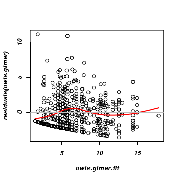
This does appear to adhere better to the homogeneity conditions.
> owls.glmer.fit <- fitted(owls.glmer)
> plot(residuals(owls.glmer) ~ owls.glmer.fit)
> rvec <- seq(min(owls.glmer.fit), max(owls.glmer.fit), l = 100)
> lines(rvec, predict(loess(residuals(owls.glmer) ~ owls.glmer.fit),
+     newdata = rvec), col = 2, lwd = 2)
> abline(h = 0, col = "gray")
-
Examine the residuals
-
Prior to examining over-dispersion, we will again explore the output.
> summary(owls.glmer)Generalized linear mixed model fit by the Laplace approximation Formula: SiblingNegotiation ~ FoodTreatment * SexParent + BroodSize + (1 | Nest) Data: owls AIC BIC logLik deviance 3529 3556 -1759 3517 Random effects: Groups Name Variance Std.Dev. Nest (Intercept) 0.172 0.415 Number of obs: 599, groups: Nest, 27 Fixed effects: Estimate Std. Error z value Pr(>|z|) (Intercept) 1.2113 0.2823 4.29 1.8e-05 *** FoodTreatmentSatiated -0.6554 0.0561 -11.68 < 2e-16 *** SexParentMale -0.0357 0.0451 -0.79 0.4285 BroodSize 0.1941 0.0656 2.96 0.0031 ** FoodTreatmentSatiated:SexParentMale 0.1301 0.0705 1.85 0.0648 . --- Signif. codes: 0 '***' 0.001 '**' 0.01 '*' 0.05 '.' 0.1 ' ' 1 Correlation of Fixed Effects: (Intr) FdTrtS SxPrnM BrodSz FdTrtmntStt -0.059 SexParentMl -0.077 0.491 BroodSize -0.950 -0.019 -0.024 FdTrtmS:SPM 0.037 -0.769 -0.605 0.022> Anova(owls.glmer)Analysis of Deviance Table (Type II tests) Response: SiblingNegotiation Chisq Df Pr(>Chisq) FoodTreatment 257.30 1 <2e-16 *** SexParent 0.17 1 0.6826 BroodSize 8.74 1 0.0031 ** FoodTreatment:SexParent 3.41 1 0.0648 . --- Signif. codes: 0 '***' 0.001 '**' 0.01 '*' 0.05 '.' 0.1 ' ' 1
Over-dispersion
It is highly likely that these data are over-dispersed (there is greater variance in the residuals than the Poisson distribution expects). We will now formally examine whether this is likely.
- Lets start by examining the ratio of actual variance to expected variance (as measured by the estimated residual degrees of freedom)
There is over 5.5 times more variance than is expected.
> rdev <- sum(residuals(owls.glmer)^2)
> #divide this by an estimate of the residual degrees of freedom (note this
> #   estimate does not account for random effects)
> mdf <- length(fixef(owls.glmer))
> rdf <- nrow(owls) - mdf  ## residual df [NOT accounting for random effects]
> rdev/rdf
[1] 5.628
-
From a Pearsons' residuals perspective:
> #explore over-dispersion from Pearson residuals perspective
> 1 - pchisq(rdev, rdf)
[1] 0
There are numerous options available for accounting for over-dispersion in the modelling phase. The diversity of these options partly reflect the different causes of over-dispersion. Two of the common reasons for over-dispersion are;
- The impacts of additional, unmeasured variables that lead to more variable replicates than otherwise expected. In these cases, quasi-Poisson or negative binomial distributions in which dispersion parameters other than 1 can be employed. These approaches have been useful for generalized linear models. More recently however, workers have advocated the use of individual random effects to attempt to soak up the additional variation as more appropriate for generalized mixed effects models.
- Greater number of zeros than would otherwise have been expected. So called "zero-inflated" data. The potential causes of zero inflation are varied and potentially complex. Zero-inflated models essentially split the problem of modelling into two parts. A Poisson model and a Binary model. The former models the data for the expected level of residual variance and the latter takes the excess zeros and treats them via a binary model.
Lets start by calculating the number (and proportion) of zeros in the data set and comparing this to the number and proportion that would be expected (given the mean)
> (owls.tab <- table(owls$SiblingNegotiation == 0))
FALSE  TRUE
  443   156
> owls.tab/sum(owls.tab)
 FALSE   TRUE
0.7396 0.2604
>
> #calculate the expected number of zeros
> owls.mu <- mean(owls$SiblingNegotiation)
> owls.mu
[1] 6.72
> cnts <- rpois(10000, owls.mu)
> owls.tab <- table(cnts == 0)
> owls.tab/sum(owls.tab)
 FALSE   TRUE
0.9989 0.0011
> nrow(owls) * (owls.tab/sum(owls.tab))
   FALSE     TRUE
598.3411   0.6589
> #very likely to be zero inflated!!
So we would have expected around 0.1% or less than one zero and yet there were 156 (or over 26% zeros). This suggests that at least some of the over-dispersion is likely to be due to zero-inflation.
Within the context of glmer, the best we can do is to attempt to model in overdispersion by incorporating individual random effects
> owls$indiv <- 1:nrow(owls)
> owls.glmerOD <- glmer(SiblingNegotiation ~ FoodTreatment * SexParent +
+     BroodSize + (1 | Nest) + (1 | indiv), family = poisson, data = owls)
As with other mixed effects models, it is worth also exploring the random structure a little more thoroughly. Currently we have fitted a random intercepts model, but we might also want to explore other combinations of random slopes to see if we can obtain an even better fit. We can do this with and without individual level random effects. The fit of all of these models can be assessed on the basis of smallest AIC and thus delta AIC.
> library(bbmle)
> owls.glmer.2 <- glmer(SiblingNegotiation ~ FoodTreatment * SexParent +
+     BroodSize + (FoodTreatment | Nest), family = poisson, data = owls)
> owls.glmer.3 <- glmer(SiblingNegotiation ~ FoodTreatment * SexParent +
+     BroodSize + (SexParent | Nest), family = poisson, data = owls)
> owls.glmer.4 <- glmer(SiblingNegotiation ~ FoodTreatment * SexParent +
+     BroodSize + (FoodTreatment * SexParent | Nest), family = poisson, data = owls)
> owls.glmer.5 <- glmer(SiblingNegotiation ~ FoodTreatment * SexParent +
+     BroodSize + (FoodTreatment * SexParent + BroodSize | Nest), family = poisson,
+     data = owls)
> owls.glmer.6 <- glmer(SiblingNegotiation ~ FoodTreatment * SexParent +
+     BroodSize + (1 | Nest) + (1 | indiv), family = poisson, data = owls)
> owls.glmer.7 <- glmer(SiblingNegotiation ~ FoodTreatment * SexParent +
+     BroodSize + (FoodTreatment | Nest) + (1 | indiv), family = poisson, data = owls)
> owls.glmer.8 <- glmer(SiblingNegotiation ~ FoodTreatment * SexParent +
+     BroodSize + (SexParent | Nest) + (1 | indiv), family = poisson, data = owls)
> owls.glmer.9 <- glmer(SiblingNegotiation ~ FoodTreatment * SexParent +
+     BroodSize + (FoodTreatment * SexParent | Nest) + (1 | indiv), family = poisson,
+     data = owls)
> owls.glmer.10 <- glmer(SiblingNegotiation ~ FoodTreatment * SexParent +
+     BroodSize + (FoodTreatment * SexParent + BroodSize | Nest) + (1 | indiv),
+     family = poisson, data = owls)
> nms <- c("Random Int", "Random Int & Random Slope (Food)", "Random Int & Random Slope (Parent)",
+     "Random Int & Random Slope (FoodxParent)", "Random Int & Random Slope (FoodxParent+BroodSize)",
+     "Over-dispersion Random Int", "Over-dispersion Random Int & Random Slope (Food)",
+     "Over-dispersion Random Int & Random Slope (Parent)", "Over-dispersion Random Int & Random Slope (FoodxParent)",
+     "Over-dispersion + Random Int & Random Slope (FoodxParent+BroodSize)")
> AICtab(owls.glmer, owls.glmer.2, owls.glmer.3, owls.glmer.4, owls.glmer.5,
+     owls.glmer.6, owls.glmer.7, owls.glmer.8, owls.glmer.9, owls.glmer.10)
              dAIC   df
owls.glmer.7     0.0 9
owls.glmer.9    14.3 16
owls.glmer.10   22.6 21
owls.glmer.6    37.8 7
owls.glmer.8    40.7 9
owls.glmer.4  1248.4 15
owls.glmer.5  1254.2 20
owls.glmer.2  1373.0 8
owls.glmer.3  1598.9 8
owls.glmer    1685.4 6
On the basis of AIC, the model that fits best, is the overdispersed model that incorporates random slopes for food treatment and random intercepts (owls.glmer.6). Note, the over-dispersed models all fit substantially better than the models that do not account for overdispersion.
> nms <- c("Random Int", "Random Int & Random Slope (Food)", "Random Int & Random Slope (Parent)",
+     "Random Int & Random Slope (FoodxParent)", "Random Int & Random Slope (FoodxParent+BroodSize)",
+     "Over-dispersion Random Int", "Over-dispersion Random Int & Random Slope (Food)",
+     "Over-dispersion Random Int & Random Slope (Parent)", "Over-dispersion Random Int & Random Slope (FoodxParent)",
+     "Over-dispersion + Random Int & Random Slope (FoodxParent+BroodSize)")
> library(lme4)
> fixedMatrix <- rbind(lmer = lme4:::fixef(owls.lmer), glmer = lme4::fixef(owls.glmer),
+     glmer2 = lme4::fixef(owls.glmer.2), glmer3 = lme4::fixef(owls.glmer.3),
+     glmer4 = lme4::fixef(owls.glmer.4), glmer5 = lme4::fixef(owls.glmer.5),
+     glmer6 = lme4::fixef(owls.glmer.6), glmer7 = lme4::fixef(owls.glmer.7),
+     glmer8 = lme4::fixef(owls.glmer.8), glmer9 = lme4::fixef(owls.glmer.9),
+     glmer10 = lme4::fixef(owls.glmer.10))
> #rownames(fixedMatrix) <- c('lmer',nms)
> sdVec <- c(lmer = attr(lme4::VarCorr(owls.lmer)[[1]], "stddev"),
+     glmer = attr(lme4::VarCorr(owls.glmer)[[1]], "stddev"), glmer2 = attr(lme4::VarCorr(owls.glmer.2)[[1]],
+         "stddev"), glmer3 = attr(lme4::VarCorr(owls.glmer.3)[[1]], "stddev"),
+     glmer4 = attr(lme4::VarCorr(owls.glmer.4)[[1]], "stddev"), glmer5 = attr(lme4::VarCorr(owls.glmer.5)[[1]],
+         "stddev"), glmer6 = attr(lme4::VarCorr(owls.glmer.6)[[1]], "stddev"),
+     glmer7 = attr(lme4::VarCorr(owls.glmer.7)[[1]], "stddev"), glmer8 = attr(lme4::VarCorr(owls.glmer.8)[[1]],
+         "stddev"), glmer9 = attr(lme4::VarCorr(owls.glmer.9)[[1]], "stddev"),
+     glmer10 = attr(lme4::VarCorr(owls.glmer.10)[[1]], "stddev"))
> #rownames(sdVec) <- c('lmer',nms)
> (compMatrix <- round(cbind(fixedMatrix, SDrandomEff = sdVec), 3))
        (Intercept) FoodTreatmentSatiated SexParentMale BroodSize
lmer          2.895                -3.627         0.237     1.218
glmer         1.211                -0.655        -0.036     0.194
glmer2        1.196                -1.111        -0.028     0.201
glmer3        1.014                -0.682        -0.046     0.233
glmer4        1.063                -1.325        -0.052     0.227
glmer5        1.204                -1.351        -0.078     0.195
glmer6        0.488                -1.116         0.017     0.282
glmer7        0.504                -1.204         0.115     0.262
glmer8        0.479                -1.147         0.007     0.286
glmer9        0.437                -1.255         0.141     0.270
glmer10       0.514                -1.271         0.113     0.259
        FoodTreatmentSatiated:SexParentMale SDrandomEff
lmer                                  0.195       1.951
glmer                                 0.130       0.415
glmer2                                0.076       0.314
glmer3                                0.136       1.206
glmer4                                0.340       0.455
glmer5                                0.366       0.600
glmer6                                0.188       0.402
glmer7                                0.015       1.462
glmer8                                0.223       0.525
glmer9                                0.116       1.116
glmer10                               0.126       0.859
> rownames(fixedMatrix) <- c("lmer", nms)
> fac <- qt(0.975, 27)
>
> fixef.low <- rbind(lmer = lme4::fixef(owls.lmer) - fac * summary(owls.lmer)@coefs[,
+     "Std. Error"], glmer = lme4::fixef(owls.glmer) - fac * summary(owls.glmer)@coefs[,
+     "Std. Error"])
> for (i in 2:10) {
+     eval(parse(text = paste("fixef.low <- rbind(fixef.low,\nglmer", i, "=lme4::fixef(owls.glmer.",
+         i, ")-fac*summary(owls.glmer.", i, ")@coefs[,'Std. Error'])", sep = "")))
+ }
>
>
> fixef.hi <- rbind(lmer = lme4::fixef(owls.lmer) + fac * summary(owls.lmer)@coefs[,
+     "Std. Error"], glmer = lme4::fixef(owls.glmer) + fac * summary(owls.glmer)@coefs[,
+     "Std. Error"])
>
> for (i in 2:10) {
+     eval(parse(text = paste("fixef.hi <- rbind(fixef.hi,lmer", i, "=lme4::fixef(owls.glmer.",
+         i, ")+fac*summary(owls.glmer.", i, ")@coefs[,'Std. Error'])", sep = "")))
+ }
>
> sdvec.low <- c(rep(NA, 11))
>
> sdvec.hi <- c(rep(NA, 11))
>
> compmat.low <- cbind(fixef.low, sdran = sdvec.low)
> compmat.hi <- cbind(fixef.hi, sdran = sdvec.hi)
>
> library(reshape)
> m <- melt(compMatrix)
> low <- melt(compmat.low)
> hi <- melt(compmat.hi)
> m$X1 <- factor(m$X1, levels = rownames(compMatrix))
> m$X2 <- factor(m$X2, levels = colnames(compMatrix))
> m$low <- low$value
> m$hi <- hi$value
> library(ggplot2)
> print(ggplot(m, aes(x = value, y = X1)) + geom_point() + geom_errorbarh(aes(xmin = low,
+     xmax = hi)) + facet_wrap(~X2, scales = "free_x") + geom_vline(x = 0, col = "red") +
+     scale_x_continuous("effect size", expand = c(0.1, 0)))
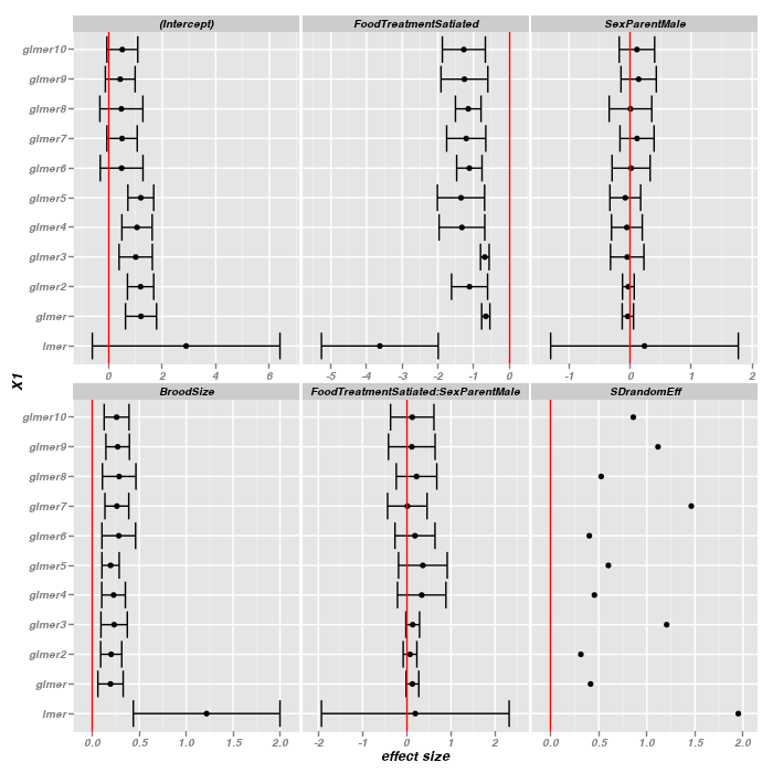
The fixed effects estimates are relatively robust across all of the over-dispersed models and indeed across all generalized linear models for that matter.
Another way to explore the fit of competing models in generalized linear models is to plot the fitted values over a histogram of the real values.
> glmer.sim1 <- simulate(owls.glmer, n = 1000)
> glmer.sim2 <- simulate(owls.glmer.2, n = 1000)
> glmer.sim3 <- simulate(owls.glmer.3, n = 1000)
> glmer.sim4 <- simulate(owls.glmer.4, n = 1000)
> glmer.sim5 <- simulate(owls.glmer.5, n = 1000)
> glmer.sim6 <- simulate(owls.glmer.6, n = 1000)
> glmer.sim7 <- simulate(owls.glmer.7, n = 1000)
> glmer.sim8 <- simulate(owls.glmer.8, n = 1000)
> glmer.sim9 <- simulate(owls.glmer.9, n = 1000)
> glmer.sim10 <- simulate(owls.glmer.10, n = 1000)
> ### Average over simulations to get predicted counts
> out <- matrix(NA, ncol = 10, nrow = 101)
> cnt <- 0:100
> for (i in 1:length(cnt)) {
+     for (j in 1:10) {
+         eval(parse(text = paste("out[i,", j, "] <- mean(sapply(glmer.sim", j,
+             ",\nFUN = function(x) {\nsum(x == cnt[i]) }))", sep = "")))
+     }
+ }
> nms <- c("Random Int", "Random Int & Random Slope (Food)", "Random Int & Random Slope (Parent)",
+     "Random Int & Random Slope (FoodxParent)", "Random Int & Random Slope (FoodxParent+BroodSize)",
+     "Over-dispersion Random Int", "Over-dispersion Random Int & Random Slope (Food)",
+     "Over-dispersion Random Int & Random Slope (Parent)", "Over-dispersion Random Int & Random Slope (FoodxParent)",
+     "Over-dispersion + Random Int & Random Slope (FoodxParent+BroodSize)")
> colnames(out) <- nms
> out.df <- data.frame(melt(out))
> out.df$X2 <- factor(out.df$X2, levels = nms)
> owls.hist <- as.data.frame(table(owls$SiblingNegotiation))
> #RColorBrewer::display.brewer.all(n=10, exact.n=FALSE)
> ggplot(data = owls.hist) + geom_bar(aes(y = Freq, x = as.numeric(Var1),
+     width = 0.1), stat = "identity", position = "identity", colour = "black",
+     fill = "black") + #geom_bar(aes(x=SiblingNegotiation),
+ #   width=0.4,position=position_dodge(width=0.5),binwidth=1,colour='black',fill='gray')+
+ geom_line(data = out.df, aes(y = value, x = X1, colour = X2, linetype = X2),
+     size = 1) + scale_x_continuous(limits = c(0, 40)) + scale_colour_brewer(palette = "Paired") +
+     opts(legend.position = "top", legend.direction = "vertical")
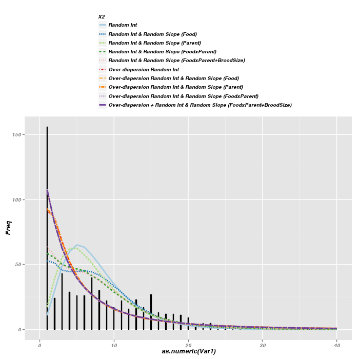
> plot(table(owls$SiblingNegotiation), ylab = "Frequency", xlab = "Sibling Negotiations",
+     lwd = 2)
> for (i in 1:10) {
+     lines(x = 0:44, y = out[1:45, i], lwd = 2, lty = 4 - (i%%4), col = RColorBrewer::brewer.pal(10,
+         "Paired")[i])
+ }
> legend("topright", legend = levels(out.df$X2), lwd = 2, lty = 4 -
+     (1:10%%4), col = RColorBrewer::brewer.pal(10, "Paired"))
The above figures are not overly clear due to the large number of lines being plotted. Nevertheless, the following conclusions can be gleaned
- The models whose simulated fitted values least approximate the actual observed count frequencies are the simple random intercepts model and the simple random intercepts/random slope for parent sex. Not surprisingly, these were also the worst fitting models on the basis of AIC
- The over-dispersed models yield better approximations than models that do not attempt to account for over-dispersion
- Although the over-dispersed models performed better in terms of model fit (AIC and simulated fitted values), it is clear that the over-dispersion is mainly due to zero-inflation and therefore even the over-dispersed models fail to fully capture the true nature of the raw counts.
Arguably, the 'best' model incorporates a random food treatment slope in addition to a random nest intercept term and a individual level random effect (glmer model 7). However, as stated, it is possible that this model would be surpassed by a model that could account for zero-inflation. Unfortunately, zero-inflated models are not supported within the context of glmer.
With this is mind, we will still examine a range of additional diagnostics in order to otherwise evaluate the appropriateness of the selected model.
> ### Get random-effects
> owls.glmer.7.re <- lme4::ranef(owls.glmer.7)
>
> opar <- par(mfrow = c(3, 2))
> hist(owls.glmer.7.re[[1]][[1]], main = "Over-dispersion", col = grey(0.6),
+     xlab = "")
> qqnorm(owls.glmer.7.re[[1]][[1]], main = "Over-dispersion")
> qqline(owls.glmer.7.re[[1]][[1]])
> hist(owls.glmer.7.re[[2]][[1]], main = "Intercept Variance", col = grey(0.6),
+     breaks = 12, xlab = "")
> qqnorm(owls.glmer.7.re[[2]][[1]], main = "Intercept Variance")
> qqline(owls.glmer.7.re[[2]][[1]])
> hist(owls.glmer.7.re[[2]][[2]], main = "Slope Variance", col = grey(0.6),
+     breaks = 12, xlab = "")
> qqnorm(owls.glmer.7.re[[2]][[2]], main = "Slope Variance")
> qqline(owls.glmer.7.re[[2]][[2]])
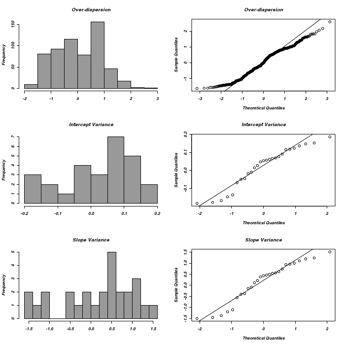
> par(opar)
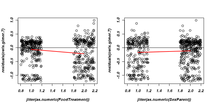
> par(mfrow = c(1, 2))
> ### Residuals on FoodTreatment
> plot(residuals(owls.glmer.7) ~ jitter(as.numeric(FoodTreatment)),
+     data = owls)
> lines(lowess(x = as.numeric(owls$FoodTreatment), y = residuals(owls.glmer.7)),
+     lwd = 2, col = "red")
> abline(h = 0)
>
> plot(residuals(owls.glmer.7) ~ jitter(as.numeric(SexParent)), data = owls)
> lines(lowess(x = as.numeric(owls$SexParent), y = residuals(owls.glmer.7)),
+     lwd = 2, col = "red")
> abline(h = 0)
Via MCMCglmm
In order to appreciate and therefore understand and use MCMCglmm, we need to take a detour into Bayesian statistics.
Bayesian statistics
Computationally robust: because Bayesian inference updates the posterior distribution one datum at a time- Design balance (unequal sample sizes) is not relevant
- Multicollinearity is not relevant
- There is no need to have expected counts greater than 5 in contingency analyses
- The stationary joint posterior distribution reflects the relative credibility of all combinations of parameter values and from which we can explore any number and combination of inferences. For example, because this stationary joint posterior distribution never changes no matter what perspective (number and type of questions) it is examined from, we can explore all combinations of pairwise comparisons without requiring adjustments designed to protect against inflating type II errors. We simply derive samples of each new parameter (e.g. difference between two groups) from the existing parameter samples thereby obtaining the posterior distribution of these new parameters.
- As we have the posterior density distributions for each parameter, we have inherent credible intervals for any parameter. That is we can state the probability that a parameter values lies within a particular range. We can also state the probability that two groups are different.
- We get the covariances between parameters and therefore we can assess interactions in multiple regression
Traditional (frequentist) statistics focus on determining the probability of obtaining the collected data, given a set of parameters. In probability notation, this can be written as:
In this philosophy, the collected data are considered just one possible subset of the population(s) and the population characteristics (parameters) of interest (such as population mean and standard deviation) are considered as fixed (each have a single, unvarying value), yet unknown properties of the population(s). The process of inference is based on approximating long-run frequencies (probability) of repeated sampling from the stationary (non-varying) population(s). This approach to statistics provides simple analytical means to objectively evaluate research questions (albeit with rigid underlying assumptions) and thus gained enormous popularity across many disciplines.
Unfortunately, the price for this elegant, computationally light system is that the associated statistical interpretations and conclusions are somewhat counter-intuitive and not quite aligned with the desired manner in which researchers would like to phrase research conclusions. Of particular note;
- probability is the probability of obtaining the collected data (or data with more extreme trends) when the null hypothesis is true (when population(s) lack any trends). P-values are commonly miss-interpreted as:
- a measure of the degree of evidence for rejecting the null hypothesis. It is a commonly held miss-belief that a smaller P-value provides greater evidence that the null hypothesis is false.
- the probability of the null hypothesis. For example, the probability that the two populations are the same is 3%, therefore they are likely to be different.
- a measure of significance - the smaller the P-value the more significant and the greater our evidence that the null hypothesis is rejected.
- the probability of a trend or effect. We cannot conclude for example, that there is a 25% probability of a trend or difference.
- P-values greater or equal to the "magic" value 0.05 are inconclusive.
- Confidence intervals define the interval that has the specified probability of containing the true, fixed unknown mean. Conclusions need to be about the interval not the population parameter.
Hence statistical conclusions drawn from traditional, frequentist approaches do not strictly pertain directly to the parameters of the populations from which data are collected, rather they relate to the collected sample(s) themselves (as well as more extreme samples). Yet surely our primary interest is in how probably our hypotheses (and thus population parameters) are rather then how probably our samples are.
Ideally then, what we actually want is the probability of obtaining a set of parameters given the data, Pr(p|y). Using very simple and well established laws of conditional probability we can derive Bayes' rule:
In essence, the probability distribution is a weighted average of the information contained in the current data and the prior expectations based on previous studies or intuition. Whilst proponents consider the ability to evaluate information within a broader and more substantive context is one of the great strengths of the Bayesian framework, opponents claim that the use or reliance of prior information has the potential to bias the outcomes. To an extent, both camps have valid points (which is perhaps why the philosophical debates continue). However, there is a practical compromise. It is possible, and indeed advisable to employ a range of priors including non-informative (or null, vague) priors. Non-informative priors are sufficiently vague (very wide, flat probability distributions from which most outcomes have similar probability densities) as to have almost no impact on the outcomes and thus resulting parameter estimates come out almost identical to those of equivalent traditional analyses. Such priors are very useful when no other priors are sensible and justifiable. By applying a range of priors, it is possible to evaluate the impact of different priors and this in itself can be a valuable form of analysis.
To qualify as a probability distribution from which certain properties (such as probabilities and confidence intervals) can be gleaned, a distribution (continuous density function) must integrate to one. That is, the total area (or volume) under the curve described by the function must equal 1. Hence, in order to convert the product of the likelihood and the prior probability into a true probability distribution it is necessary to normalize this unnormalized posterior distribution by division with Pr(y), the normalizing constant or "marginal likelihood". Pr(y) is the probability of our data considering the model and is determined by summing across all possible parameter values weighted by the strength of belief of those parameters. Unfortunately, this typically involves integration of irregular high-dimensional functions (the more parameters, the more dimensions), and is thus usually intractable.
One way to keep the math simple is to use likelihood functions with "conjugate" prior functions to ensure that the prior function is of the same form as the prior function. It is also possible to substitute the functions with approximations that simplify the algebra.
Markov Chain Monte Carlo sampling
Markov Chain Monte Carlo (MCMC) algorithms provide a powerful, yet relatively simple means of generating samples from high-dimensional distributions. Whilst there are numerous specific MCMC algorithms, they all essentially combine a randomization routine (Monte Carlo component) with a routine that determines whether or not to accept or reject randomizations (Markov Chain component) in a way that ensures that the samples are drawn from multidimensional space proportional to their likelihoods such that the distribution of these samples (posterior probability distribution) reflects their likelihood in high-dimensional space. Given a sufficiently large number of simulations, the resulting samples should exactly describe the target probability distribution and thereby allow the full range of parameter characteristics to be derived.
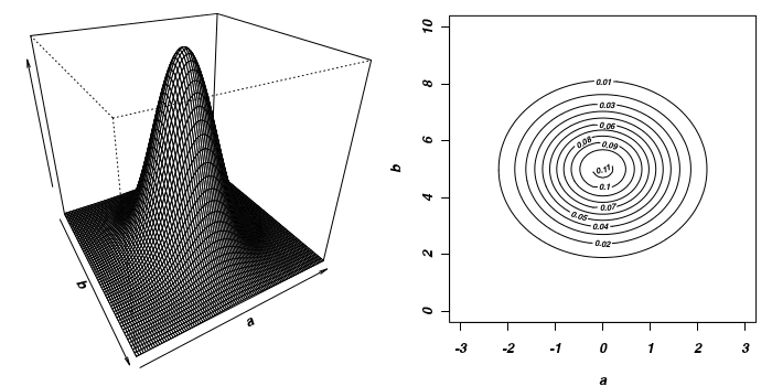
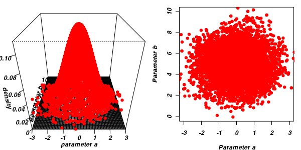
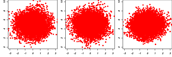
To illustrate the mechanics of MCMC sampling, I will contrive a very simple scenario in which we have two parameters (α and β). I will assume infinitely vague priors on both parameters and thus the density function from which to draw samples will simply be the likelihood density function for these parameters. For simplicity sake, this likelihood function will be a multivariate normal distribution for the two parameters with values of α=0 (sd=1) and β=5 (sd=2). The following two graphics provide two alternative views (perspective view and contour view) of this likelihood density function.
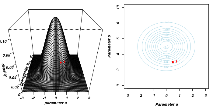
The specific MCMC algorithm that I will describe is the Metropolis-Hastings algorithm and I will do so as much as possible via visual aids. Initially a location (coordinates) in multi-dimensional space (in this case 2-D) corresponding to a particular set of parameter values is chosen as the starting location. We will start with the coordinates (α=0.5, β=-0.5), yet make the point that if we collect enough samples, the importance of the initial starting configuration will diminish.
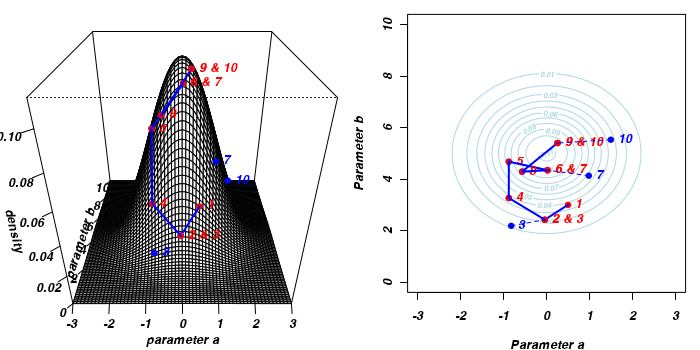
Now lets move to another random sampling location. To do so, we will move a random multivariate distance and direction from the current location based on the coordinates of a single random location drawn from a multivariate normal distribution centered around zero. The ratio of probabilities (heights on the perspective diagram) corresponding to the new and previous locations is then calculated and this ratio effectively becomes the probability of accepting the new location. For example, the probability associated with the initial location was approximately 0.037 and the probability associated with the new location is 0.019. The probability of moving is therefore 0.019/0.037=0.513. There is just over 50% chance of moving. A random number between 0 and 1 is then drawn from a uniform distribution. If this number is greater than the ratio described above, the new location is rejected and the previous location is resampled. However, if the number is less than the ratio, then the new location is accepted and parameter values are stored from this new location.

The sampling chain continues until a predefined number of iterations have occurred.
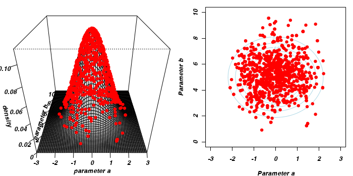
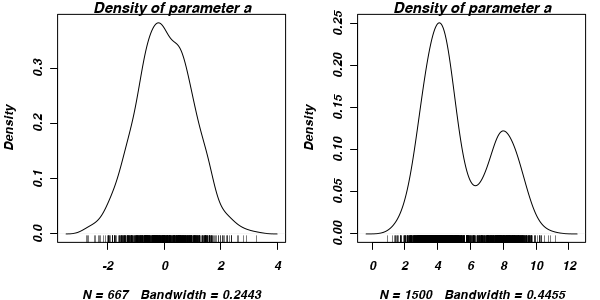
The collected samples, in this case 1000 samples for α and 1000 for β, can then be used to calculate a range of characteristics.
> colnames(params) <- c("a", "b")
> apply(params, 2, mean)
      a       b
-0.0309  5.2243
> apply(params, 2, sd)
     a      b
0.8793 1.4364
- Perhaps the posterior distribution (represented by the red dots) had not yet stabilized.
That is, perhaps the shape of the posterior distribution was still changing slightly with each additional sample collected.
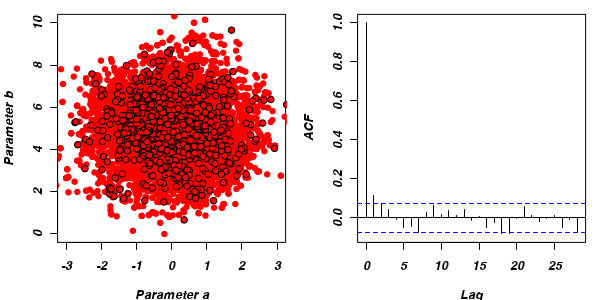
The chain had not yet completely sampled the entire surface in approximate proportion to the densities. If so, then collecting substantially more samples could address this. Lets try 10,000.
       a        b
-0.02837  4.99913
    a     b
1.011 1.423
The "sharper" the features (and more isolated islands) in the multidimensional profile, the more samples will be required in order to ensure that the Markov chain traverses (mixes across) all of the features. One of the best ways of evaluating whether or not sufficient samples have been collected is with a trace plot. Trace plots essentially display the iterative history of MCMC sequences. Ideally, the trace plot should show no trends, just consistent random noise around a stable baseline. Following are three trace plots that depict an adequate number samples, inadequate number of samples and insufficient mixing across all features.

-
The drawback of a Markov Chain is that the samples are not independent of one another. In a sense, its strength (the properties that allow it to simulate in proportion to the density) can also be a weakness in that consecutive samples are likely to be very similar (non-independent) to one another. It turns out that there is a very simple remedy for this however. Rather than store every single sample, we can thin the sample set by skipping over (not storing) some of the samples. For example, we could nominate to store every second, or fifth or tenth etc sample. The resulting samples will thence be more independent of one another. Note however, that the sample will be smaller by a factor of the thinning value and thus it will be necessary to perform more iterations.
To illustrate autocorrelation and thinning, we will run the MCMC simulations twice, the first time with no thinning and a second time with a thinning factor of 10.
Non-thinned (stored) samples are depicted as circles with black borders. Associated with each chain of simulations, is an autocorrelation function (ACF) plot which represents the degree of correlation between all pairs of samples separated by progressively larger lags (number of samples).
Thinning factor = 1Thinning factor = 10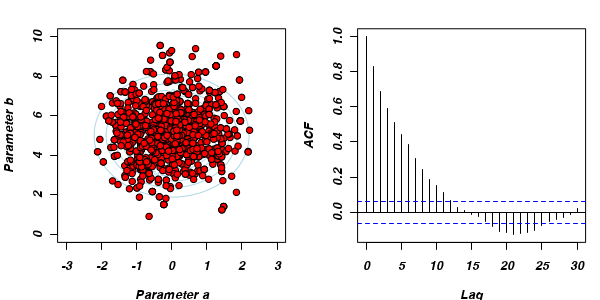 For the un-thinned samples, the autocorrelation at lag 1 (adjoining pairs of samples) is over 0.8 (80%) indicating a very high degree of non-independence. Ideally, we would like to aim for a lag 1 autocorrelation value no greater than 0.1. According to the ACF plot associated with the un-thinned simulation chain, to achieve a lag 1 autocorrelation value of no greater than 0.1 would require a sample separation (thinning) of greater than 10. Indeed, the second simulation chain had a thinning factor of 10 (only retained every 10th sample) and still has a lag 1 autocorrelation value greater than 0.1 (although this is may now be because it is based on a much smaller sample size). To be sure, we could re-simulate the chain again with a 15-fold thinning but with 10 times more iterations (a total of 10,000).
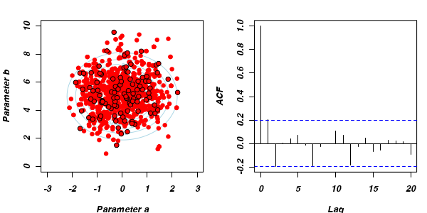
- Although the importance of the starting configuration (initial coordinates) should eventually diminish as the stochastic walk traverses more and more of the profile, for shorter chains, the initial the initial path traversed is likely to exert a pull on the sample values. Of course, substantially increasing the number of iterations of the chain will substantially increase the time it takes to run the chain. Hence, it is common to define a burnin interval at the start of the chain. This defines the number of initial iterations that are ignored (samples not retained). Generally, ignoring the first 10% of iterations should be sufficient. In the current artificial example, this is unlikely to be an issue as the density distribution has very blunt, connected features.
Eventually (given enough iterations), the MCMC chain should sample the entire density profile and the resulting posterior distribution should converge (produce relatively invariant outcomes) on a stationary distribution (the target distribution).
Unlike models fitted via maximum likelihood (which stop iterating when the improvement in log-likelihood does not exceed a pre-defined value - at which point they have usually converged), MCMC chains do not have a stopping criterion. Rather, the analyst must indicate the number of iterations (simulations) to perform. The number of iterations is always a compromise between convergence and time. The more iterations, the better the mixing and coverage, the greater the likelihood of convergence, yet the greater the time it takes to complete the analysis.
Given that accuracy of the chain is dependent on convergence, it is critical that the plausibility of convergence be evaluated in order to be confident in the reliability of the Markov Chain Monte Carlo sampling and thus the characteristics of the returned samples. There are numerous diagnostics available, each of which focusses on different indicators of non-convergence;
- Trace plots - as described above, trace plots for each parameter offer visual indicators of issues with the mixing and coverage of the samples collected by the chain as well as the presence of a starting configuration impact. In addition to the lack of drift, the residuals (sometimes called units) should be centered around 0. Positive displacement of the residuals can be an indication of zero-inflation (response having more zeros that the modelling distribution should expect).
- Plots of the posterior distribution (density or histograms) of each parameter. The basic shape of these plots should follow the approximate expected joint probability distribution (between family modelled in determining likelihood and prior). In our contrived example, this should be a normal distribution. Hence, obviously non-normal (particularly bimodal) distributions would suggest that the chain has not yet fully mixed and converged on a stationary distribution. In the case of expected non-normal distributions, the density plots can also serve to remind us that certain measures of location and spread (such as mean and variance) might be inadequate characterizations of the population parameters.
- Autocorrelation - correlation between successive samples (as a result of way the Markov Chain spreads) are useful for determining the appropriate amount of thinning required to generate a well mixed series of samples. Autocorrelation can be explored visually (in a plot such as that illustrated earlier) or numerically by simply exploring the autocorrelation values at a range of lags.
-
The Geweke diagnostic (and Geweke-Brooks plot) compares the means (by a standard Z-score) of two non-overlapping sections of the chain
(by default the first 10% and the last 50%) to explore the likelihood that the samples from the two sections come from the same stationary distribution. In the plot, successively larger numbers of iterations are dropped from the start of the samples (up to half of the chain) and the resulting Z-scores are plotted against the first iteration in the starting segment. Substantial deviations of the Z-score from zero (those outside the horizontal critical confidence limits) imply poor mixing and a lack of convergence. The Geweke-Brooks plot is also particularly useful at diagnosing a lack of mixing due o the initial configuration and how long the burnin phase should be.

-
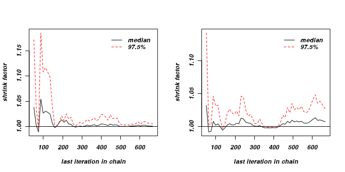
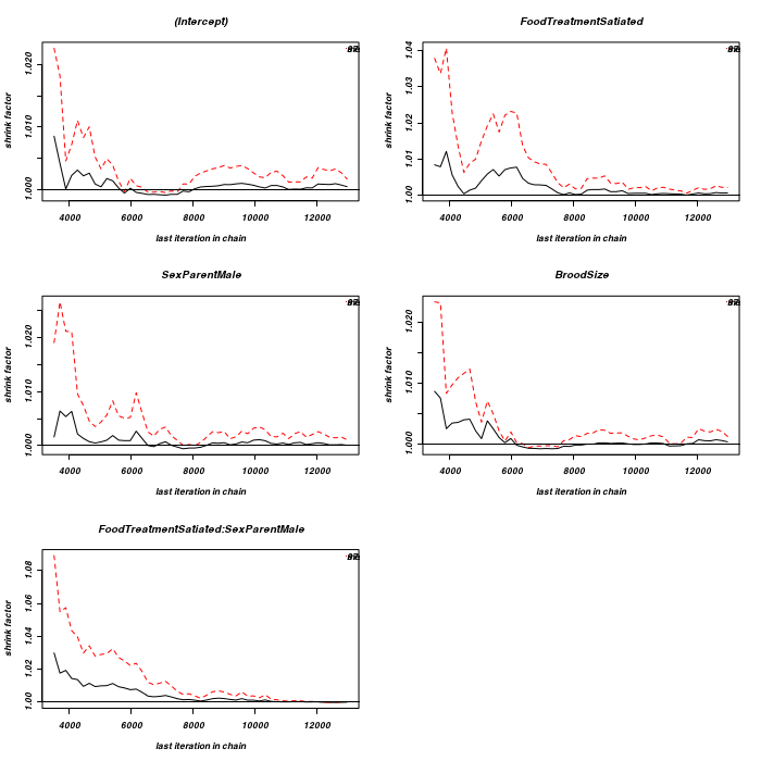
The Gelman and Rubin diagnostic essentially calculates the ratio of the total variation within and between multiple chains to the within chain variability (this ratio is called the Potential Scale Reduction Factor). As the chain progresses (and samples move towards convergence) the variability between chains should diminish such that the scale reduction factor essentially measures the ratio of the within chain variability to itself. At this point (when the potential scale reduction factor is 1), it is likely that any one chain should have converged. When the potential scale reduction factor is greater than 1.1 (or more conservatively 1.2), we should run the chain(s) for longer to improve convergence.
Clearly, in order to calculate the Gelman and Rubin diagnostic and plot, it is necessary to run multiple chains. When doing so, it is advisable that different starting configurations be used for each chain.
-
A Raftery and Lewis diagnostic estimates the number of iterations and the burnin length required to have a
given probability (95%) of posterior quantile (0.025) accuracy (0.005). In the following, I will show the Raftery and Lewis diagnostic from a sample length of 1000 (which it considers below the minimum requirements for the quantile, probability and accuracy you have nominated) and this will be followed by diagnostics from a longer chain (40,000 iterations with a thinning factor of 10). In the latter case, for each parameter it lists the burnin length (M), number of MCMC iterations (N), minimum number of (uncorrelated) samples to construct this pilot and I (the proportional increase in necessary iterations due to autocorrelation). Values of I greater than 5 indicate substantial autocorrelation.
Quantile (q) = 0.025
Accuracy (r) = +/- 0.005
Probability (s) = 0.95

You need a sample size of at least 3746 with these values of q, r and s
Quantile (q) = 0.025 Accuracy (r) = +/- 0.005 Probability (s) = 0.95 Burn-in Total Lower bound Dependence (M) (N) (Nmin) factor (I) 4 4782 3746 1.28 5 5894 3746 1.57 - The Heidelberg and Welch diagnostic tests a null hypothesis that the Markov chain is from a stationary distribution. The test evaluates the accuracy of the estimated means after incremently discarding more and more (10%, 20%, 30% up to 50%) of the chain. The point at which the null hypothesis is accepted marks the number of iterations required to keep. If the null hypothesis is not accepted by the time 50% of the chain has been discarded, it suggests that more MCMC iterations are required to reach a stationary distribution and to estimate the mean with sufficient accuracy. For the portion of the chain that passed (null hypothesis accepted), the sample mean and 95% confidence interval are calculated. If the ratio of the mean to 95% interval is greater than 0.1, then the mean is considered accurate otherwise a longer overall chain length is recommended. Note, this diagnostic is misleading for residuals or any other parameters whose means are close to zero. Whilst this diagnostic can help trim chains to gain speed, in practice it is more useful for just verifying that the collected chain is long enough.
  Stationarity start     p-value
  test         iteration
a passed       1         0.365
b passed       1         0.668

  Halfwidth Mean   Halfwidth
  test
a failed    0.0262 0.0856
b passed    5.0083 0.1390
     Stationarity start     p-value
     test         iteration
[,1] passed       1         0.254
[,2] passed       1         0.875

     Halfwidth Mean   Halfwidth
     test
[,1] failed    -0.017 0.0368
[,2] passed     5.003 0.0564
Although MCMC algorithms have their roots in the Bayesian paradigm, they are not exclusively bound to Bayesian analyses. Philosophical arguments aside, MCMC sampling algorithms provide very powerful ways to tackling otherwise intractable statistical models. Indeed, it is becoming more and more for MCMC sampling to employed alongside vague (non-informative) priors to fit models that are otherwise not analytically compliant or convergent.
Priors
Bayesian analyses incorporate prior expectations about the parameters being estimated (fixed effects, random effects and residuals). Even when no prior information is available, priors must still be defined to make use of MCMC sampling techniques. In such cases, non-informative priors are typically defined. Generally these are:- fixed effects - normal (Gaussian) or even uniform distributions with very wide variances. Very wide variances essentially mean that the fixed effects priors have little or no influence on the posterior distributions of the parameters. A sensible non-informative prior would be centered around zero with a large (108) variance.
- Random effects - inverse Wishart distribution. The inverse Wishart distribution is defined by two parameters (
V- representing a sort of location measure, the value at its peak; andnu- the degree of belief parameter). Asnuapproaches infinity (complete belief), the peak of the Wishart distribution approachesV. A sensible non-informative prior would be a Wishart distribution withV=1, nu=0.002.
We will approach the process of model building in MCMCglmm in a similar manner to that adopted for glmer
That is, we will start with a relatively simple model and gradually build complexity before evaluating and selecting the 'best' model from amongst the candidates.
Note that MCMCglmm fitted models always anticipate and attempt to account for over-displacement.
> library(MCMCglmm)
Basic model fitting
MCMCglmm follows much the same formula and fitting syntax as lmer.
It uses a MCMC Metropolis-Hastings sampling chain with the following defaults;
- 13,000 iterations (
nitt=13000) - 3000 burnin iterations (
burnin=1000) - 10 fold thinning (
thin=10) - non-informative priors
- R-structure - residual (units) - Inverse-Wishart distribution with V=1 and nu=0.002
- G-structure - random effects - Inverse-Wishart distribution with V=1 and nu=0
- B-structure - fixed effects - multivariate Guassian or ... mu=0 and large V
Lets start by fitting the null model under default conditions
> owls.MCMCglmm <- MCMCglmm(SiblingNegotiation ~ 1, random = ~Nest,
+     family = "poisson", data = owls, verbose = FALSE)
Now lets fit a model roughly equivalent to that considered most useful via lmer.
> owls.MCMCglmm2 <- MCMCglmm(SiblingNegotiation ~ FoodTreatment * SexParent +
+     BroodSize, random = ~Nest, family = "poisson", data = owls, verbose = FALSE)
Having fitted a very basic generalized linear mixed effects model (owls.MCMCglmm2 with a MCMC sampler, there
are a number of convergence diagnostics that we need to explore (in addition to other measures of model fit) in order to be confident that he Markov Chain converged on a stationary posterior distribution and thus to be confident in the accuracy and reliability of the returned samples. However, prior to exploring these diagnostics, it is worth getting a sense for the structure and contents of the returned fitted object.
> attributes(owls.MCMCglmm2)
$names
 [1] "Sol"        "Lambda"     "VCV"        "CP"         "Liab"       "Fixed"      "Random"
 [8] "Residual"   "Deviance"   "DIC"        "X"          "Z"          "XL"         "error.term"
[15] "family"

$class
[1] "MCMCglmm"
The most important components of this structure are;
- Sol - the posterior distribution (samples) of the mixed modelling equation solutions (fixed effects). It is a matrix comprising of samples for each parameter in columns and retained sample in rows
- VCV - the posterior distribution (samples) of the covariance matrices
- Deviance - the deviance of the fitted model
- DIC - the deviance information criterion
Given sufficient iterations, the chain WILL eventually converge to a stationary distribution for each estimatable parameter, which will also be the target distribution for each parameter.
However, in fitting the MCMCglmm model, we nominated the length of the Markov Chain (13,000) and the number of samples to retain ((13,000-3,000)/10 = 1000). There are numerous diagnostics to help us judge whether the chain is likely to have converged on stationary distributions.
- Examine the traces (trace plots of the iterative history of MCMC sequences) of sampled output as well as the posterior distribution for each fixed and random term
The traces indicate reasonably good convergence - the noise does not appear to drift majorly. This suggests that the chain has probably mixed well and converged. There are however, two points of note.
> plot(as.mcmc(owls.MCMCglmm2$Sol), ask = FALSE)


> plot(as.mcmc(owls.MCMCglmm2$VCV), ask = FALSE)
- The trace and density of Nest (the random effect) is asymmetrical. Consequently, a mean value is perhaps not the most representative measure of Nest effects. Median or mode are arguably more appropriate measures of location. Likewise, quantiles are more appropriate than standard deviations as measures of spread.
- The trace and density of units (replicates) is not centered around zero. Rather they are positively displaced and centered around a value of approximately 1.3. This is likely to suggest that the model failed to account fully for zero-inflation.
-
Autocorrelation - correlation between samples at different lags.
Note by default,
MCMCglmmthins to every 10th sample and has a burnin of 3000 samples.Focussing on lags greater than zero, all correlations are less (in magnitude) than 0.1 implying no major issues with autocorrelation for the thinning factor used.> autocorr(owls.MCMCglmm2$Sol), , (Intercept) (Intercept) FoodTreatmentSatiated SexParentMale BroodSize Lag 0 1.00000 -0.147588 -0.179788 -0.92813 Lag 10 0.05689 0.007909 -0.034003 -0.05106 Lag 50 0.05428 0.018346 -0.005017 -0.06293 Lag 100 -0.06045 -0.024823 -0.053205 0.04784 Lag 500 0.03419 0.011083 0.034823 -0.04466 FoodTreatmentSatiated:SexParentMale Lag 0 0.08580 Lag 10 0.01444 Lag 50 -0.02421 Lag 100 0.05393 Lag 500 -0.03037 , , FoodTreatmentSatiated (Intercept) FoodTreatmentSatiated SexParentMale BroodSize Lag 0 -0.14759 1.000000 0.527683 -0.02519 Lag 10 0.03069 0.100640 0.016591 -0.02881 Lag 50 -0.03418 0.003722 0.011433 0.03243 Lag 100 0.02778 -0.049205 -0.037282 -0.01462 Lag 500 -0.03577 -0.006222 0.009902 0.04310 FoodTreatmentSatiated:SexParentMale Lag 0 -0.742807 Lag 10 -0.058966 Lag 50 -0.025184 Lag 100 0.036363 Lag 500 0.005672 , , SexParentMale (Intercept) FoodTreatmentSatiated SexParentMale BroodSize Lag 0 -0.17979 0.527683 1.000000 -0.04301 Lag 10 0.01525 0.003638 0.004742 -0.01810 Lag 50 -0.03211 0.045635 0.020910 0.02494 Lag 100 0.05972 -0.062516 -0.055364 -0.03769 Lag 500 0.04757 0.005687 0.019479 -0.05415 FoodTreatmentSatiated:SexParentMale Lag 0 -0.641269 Lag 10 -0.003901 Lag 50 -0.022668 Lag 100 0.045828 Lag 500 -0.004722 , , BroodSize (Intercept) FoodTreatmentSatiated SexParentMale BroodSize Lag 0 -0.92813 -0.025190 -0.043013 1.00000 Lag 10 -0.05438 0.003478 0.051706 0.04562 Lag 50 -0.05309 -0.019949 0.007477 0.05457 Lag 100 0.03479 0.040451 0.074106 -0.02904 Lag 500 -0.05055 -0.008917 -0.030637 0.05876 FoodTreatmentSatiated:SexParentMale Lag 0 0.05478 Lag 10 -0.03079 Lag 50 0.02626 Lag 100 -0.07191 Lag 500 0.02139 , , FoodTreatmentSatiated:SexParentMale (Intercept) FoodTreatmentSatiated SexParentMale BroodSize Lag 0 0.085798 -0.742807 -0.641269 0.054784 Lag 10 -0.013395 -0.076558 -0.026765 0.022038 Lag 50 0.032834 0.001523 -0.003225 -0.029165 Lag 100 -0.030713 0.052790 0.028928 0.014701 Lag 500 -0.009837 0.022094 -0.009735 0.006111 FoodTreatmentSatiated:SexParentMale Lag 0 1.0000000 Lag 10 0.0646318 Lag 50 -0.0007688 Lag 100 -0.0271614 Lag 500 -0.0213728> autocorr(owls.MCMCglmm2$VCV), , Nest Nest units Lag 0 1.00000 0.011453 Lag 10 0.09750 0.079173 Lag 50 -0.02195 0.002512 Lag 100 0.04763 0.006771 Lag 500 -0.01954 -0.033763 , , units Nest units Lag 0 0.011453 1.00000 Lag 10 0.085802 0.27650 Lag 50 0.043818 0.04843 Lag 100 0.005879 -0.01395 Lag 500 -0.042111 -0.03086 -
The Geweke diagnostic (and plot) compares the means of two non-overlapping sections of the chain
(by default the the first 10% and the last 50%)
to explore the likelihood that the samples from the two sections come from the same distribution.
Successively larger numbers of iterations are dropped from the start of the samples (up to half of the chain).
There is very little evidence of insufficient mixing for any of the parameters with the possible exception of the food treatment effect, and then it is only mild and not really worth worrying about.
> geweke.plot(owls.MCMCglmm2$Sol)
> geweke.plot(owls.MCMCglmm2$VCV)
-
We can also explore convergence by examining Potential scale reduction factors and a Gelman and Rubin diagnostic plot.
The Gelman and Rubin diagnostics essentially calculates the ratio of the total variation within and between multiple chains to the within chain variability.
As the chain progresses (as the samples converge) the variability between chains should diminish such that the scale reduction factor essentially measures the ratio of the within chain variability with itself.
At this point (when the scaling factor is 1), it is likely that any one chain should have converged.
Ratios quickly converge to values around 1. Even when the ratios deviate from 1, they remain well under 1.1. Hence, again there is no evidence that the chain has not converged on a stationary posterior distribution.
> for (i in 1:5) {
+     eval(parse(text = paste("fit.", i, "<-MCMCglmm(SiblingNegotiation~FoodTreatment*SexParent+BroodSize,random=~Nest, family='poisson', data=owls,verbose=FALSE)",
+         sep = "")))
+ }
> mcmc.list <- mcmc.list(list(fit.1$Sol, fit.2$Sol, fit.3$Sol, fit.4$Sol,
+     fit.5$Sol))
> gelman.plot(mcmc.list)
-
Raftery and Lewis diagnostic estimates the number of samples required for each parameter so as to have a given probability (95%) of posterior quantile (0.025) accuracy (0.005).
These results suggest that there are insufficient samples to achieve the nominated characteristics. That said, it is the only diagnostic out of the applied set that is coming to this conclusion. Consequently, we will ignore it!
> raftery.diag(owls.MCMCglmm2)Quantile (q) = 0.025 Accuracy (r) = +/- 0.005 Probability (s) = 0.95 You need a sample size of at least 3746 with these values of q, r and s
-
The Heidelberg and Welch diagnostic tests a null hypothesis that the Markov chain is from a stationary distribution.
It essentially tests whether the chain length was sufficient to reach stationary and to estimate the mean with sufficient accuracy. It also compares estimates of means to half the value of standard deviations.
With the exception of the sex of the parent effect half-way test, all tests passed. The one failure is not of great concern considering that its mean was very close to zero. The test for units should normally be expected to fail the half-way test (as it should have a mean close to zero). The fact that it did not fail is also support for zero-inflation.
> heidel.diag(owls.MCMCglmm2$Sol)Stationarity start p-value test iteration (Intercept) passed 1 0.2617 FoodTreatmentSatiated passed 1 0.3031 SexParentMale passed 1 0.1783 BroodSize passed 1 0.2171 FoodTreatmentSatiated:SexParentMale passed 101 0.0895 Halfwidth Mean Halfwidth test (Intercept) passed 0.4837 0.03039 FoodTreatmentSatiated passed -1.1265 0.01335 SexParentMale failed 0.0188 0.01083 BroodSize passed 0.2808 0.00727 FoodTreatmentSatiated:SexParentMale passed 0.1877 0.01862> heidel.diag(owls.MCMCglmm2$VCV)Stationarity start p-value test iteration Nest passed 1 0.469 units passed 1 0.647 Halfwidth Mean Halfwidth test Nest passed 0.289 0.0104 units passed 1.286 0.0110
Conclusions - most of the above diagnostics broadly concur that the samples have converged on stationary distributions within the 13000 iterations.
Of course we should also explore how well the model fits the data using the typical residual diagnostics.
Although MCMCglmm does not have a function for extracting the residuals, it is possible to calculate residuals
by subtracting predicted values from the raw data. The MCMCglmm package includes a predict function, however Jarrod Hadfield does warn that it is still experimental. We can always approximate (this method neglects the random factors) the predicted values by multiplying the returned coefficients by the fixed model matrix (and then expressing the values in the response scale).
forward to calculate them from the raw data and the predicted values.
> pred <- predict(owls.MCMCglmm2)
> res <- owls$SiblingNegotiation - pred
> plot(res ~ pred)

> #alternatively, a manual approximation
> mat <- owls.MCMCglmm2$X
> pred <- poisson()$linkinv(aa)
> aa <- as.vector(colMeans(owls.MCMCglmm2$Sol) %*% t(mat))
> pred <- poisson()$linkinv(aa)
> res <- owls$SiblingNegotiation - pred
> plot(res ~ pred)

Given that the trace and density diagrams indicated that there might be a zero-inflation issue,
it might now be worth exploring a zero-inflated Poisson model.
MCMCglmm supports zero inflated, zero altered, zero truncated and hurdle models for Poisson distributions and zero-inflated models for binomial distributions. When specifying a zero-inflated model, it is necessary to also define the residual covariance structure. There are two reserved terms within MCMCglmm;
- trait - indexes columns of the response variable. This is to accommodate multivariate responses as well as zero-inflated models (which effectively model the response variable twice).
- units - indexes rows of the response variable (and therefore represents the replicates)
- idv - fits constant variances across each component of the formula
- idh - fits different variances across each component of the formula
- us - fits different variances and covariances across each component of the formula
So lets fit the zero-inflated Poisson model with default MCMC behaviour, default priors and default variance-covariance for the G-structures.
> owls.MCMCglmm3 <- MCMCglmm(SiblingNegotiation ~ FoodTreatment * SexParent +
+     BroodSize, random = ~Nest, family = "zipoisson", data = owls, rcov = ~idh(trait):units,
+     verbose = FALSE)
Lets now explore the traces and density plots for the fixed effects.
> plot(as.mcmc(owls.MCMCglmm3$Sol), ask = FALSE)


> plot(as.mcmc(owls.MCMCglmm3$VCV), ask = FALSE)

It would appear that the chain has not converged with respect to zero-inflated residuals.
> owls.MCMCglmm3a <- MCMCglmm(SiblingNegotiation ~ FoodTreatment *
+     SexParent + BroodSize, random = ~Nest, family = "zipoisson", data = owls,
+     rcov = ~idh(trait):units, verbose = FALSE, nitt = 1e+05)
> plot(as.mcmc(owls.MCMCglmm3a$VCV), ask = FALSE)

> prior <- list(R = list(V = diag(2), n = 1.002, fix = 2), G = list(G1 = list(V = 1,
+     n = 0.002), G2 = list(V = 1, n = 0.002)))
> owls.MCMCglmm3a <- MCMCglmm(SiblingNegotiation ~ FoodTreatment *
+     SexParent + BroodSize, random = ~idh(at.level(FoodTreatment, 2)):Nest +
+     idh(at.level(FoodTreatment, 1)):Nest, family = "zipoisson", data = owls,
+     rcov = ~idh(trait):units, verbose = FALSE, prior = prior)
> prior <- list(R = list(V = diag(2), n = 1.002), G = list(G1 = list(V = diag(2),
+     n = 1.002), G2 = list(V = diag(2), n = 1.002)))
> owls.MCMCglmm3a <- MCMCglmm(SiblingNegotiation ~ FoodTreatment *
+     SexParent + BroodSize, random = ~idh(FoodTreatment):Nest + idh(SexParent):Nest,
+     family = "zipoisson", data = owls, rcov = ~idh(trait):units, verbose = FALSE,
+     prior = prior)
> plot(as.mcmc(owls.MCMCglmm3a$Sol), ask = FALSE)


> plot(as.mcmc(owls.MCMCglmm3a$VCV), ask = FALSE)


> #random slope for BroodSize
> prior <- list(R = list(V = diag(2), n = 1.002, fix = 2), G = list(G1 = list(V = 1,
+     n = 0.002), G2 = list(V = diag(2), n = 1.002)))
> owls.MCMCglmm3a <- MCMCglmm(SiblingNegotiation ~ FoodTreatment *
+     SexParent + BroodSize, random = ~idh(at.level(FoodTreatment, 2)):Nest +
+     idh(at.level(FoodTreatment, 1) + at.level(FoodTreatment, 1):BroodSize):Nest,
+     family = "zipoisson", data = owls, rcov = ~idh(trait):units, verbose = FALSE,
+     prior = prior)
> plot(as.mcmc(owls.MCMCglmm3a$Sol), ask = FALSE)


> plot(as.mcmc(owls.MCMCglmm3a$VCV), ask = FALSE)


>
>
> prior <- list(R = list(V = diag(2), n = 1.002), G = list(G1 = list(V = diag(2),
+     n = 1.002)))
> owls.MCMCglmm3a <- MCMCglmm(SiblingNegotiation ~ FoodTreatment *
+     SexParent + BroodSize, random = ~idh(FoodTreatment):Nest, family = "zipoisson",
+     data = owls, rcov = ~idh(trait):units, verbose = FALSE, prior = prior)
>
> prior <- list(R = list(V = diag(2), n = 1.002), G = list(G1 = list(V = 1,
+     n = 1.002)))
> owls.MCMCglmm3a <- MCMCglmm(SiblingNegotiation ~ FoodTreatment *
+     SexParent + BroodSize, random = ~Nest, family = "zipoisson", data = owls,
+     rcov = ~idh(trait):units, verbose = FALSE, prior = prior)
> owls.MCMCglmm4 <- MCMCglmm(SiblingNegotiation ~ FoodTreatment * SexParent +
+     BroodSize, random = ~FoodTreatment:Nest, family = "zipoisson", data = owls,
+     rcov = ~idh(trait):units, verbose = FALSE)
> plot(as.mcmc(owls.MCMCglmm4$Sol), ask = FALSE)


> plot(as.mcmc(owls.MCMCglmm4$VCV), ask = FALSE)

> owls.MCMCglmm5 <- MCMCglmm(SiblingNegotiation ~ FoodTreatment * SexParent +
+     BroodSize, random = ~FoodTreatment:Nest + SexParent:Nest, family = "zipoisson",
+     data = owls, rcov = ~idh(trait):units, verbose = FALSE)
> plot(as.mcmc(owls.MCMCglmm5$Sol), ask = FALSE)


> plot(as.mcmc(owls.MCMCglmm5$VCV), ask = FALSE)

> owls.MCMCglmm6 <- MCMCglmm(SiblingNegotiation ~ FoodTreatment * SexParent +
+     BroodSize, random = ~idh(FoodTreatment):Nest, family = "zipoisson", data = owls,
+     rcov = ~idh(trait):units, verbose = FALSE)
> plot(as.mcmc(owls.MCMCglmm6$Sol), ask = FALSE)


> plot(as.mcmc(owls.MCMCglmm6$VCV), ask = FALSE)

> owls.MCMCglmm7 <- MCMCglmm(SiblingNegotiation ~ FoodTreatment * SexParent +
+     BroodSize, random = ~idh(FoodTreatment):Nest + idh(SexParent):Nest, family = "zipoisson",
+     data = owls, rcov = ~idh(trait):units, nitt = 25000)
                      MCMC iteration = 0

  Acceptance ratio for latent scores = 0.000492

                      MCMC iteration = 1000

  Acceptance ratio for latent scores = 0.332846

                      MCMC iteration = 2000

  Acceptance ratio for latent scores = 0.323688

                      MCMC iteration = 3000

  Acceptance ratio for latent scores = 0.325503

                      MCMC iteration = 4000

  Acceptance ratio for latent scores = 0.352274

                      MCMC iteration = 5000

  Acceptance ratio for latent scores = 0.346883

                      MCMC iteration = 6000

  Acceptance ratio for latent scores = 0.344970

                      MCMC iteration = 7000

  Acceptance ratio for latent scores = 0.330359

                      MCMC iteration = 8000

  Acceptance ratio for latent scores = 0.353853

                      MCMC iteration = 9000

  Acceptance ratio for latent scores = 0.371958

                      MCMC iteration = 10000

  Acceptance ratio for latent scores = 0.377726

                      MCMC iteration = 11000

  Acceptance ratio for latent scores = 0.377656

                      MCMC iteration = 12000

  Acceptance ratio for latent scores = 0.375673

                      MCMC iteration = 13000

  Acceptance ratio for latent scores = 0.382446

                      MCMC iteration = 14000

  Acceptance ratio for latent scores = 0.383447

                      MCMC iteration = 15000

  Acceptance ratio for latent scores = 0.376598

                      MCMC iteration = 16000

  Acceptance ratio for latent scores = 0.375948

                      MCMC iteration = 17000

  Acceptance ratio for latent scores = 0.374237

                      MCMC iteration = 18000

  Acceptance ratio for latent scores = 0.374513

                      MCMC iteration = 19000

  Acceptance ratio for latent scores = 0.370593

                      MCMC iteration = 20000

  Acceptance ratio for latent scores = 0.363344

                      MCMC iteration = 21000

  Acceptance ratio for latent scores = 0.361314

                      MCMC iteration = 22000

  Acceptance ratio for latent scores = 0.362297

                      MCMC iteration = 23000

  Acceptance ratio for latent scores = 0.364356

                      MCMC iteration = 24000

  Acceptance ratio for latent scores = 0.353112

                      MCMC iteration = 25000

  Acceptance ratio for latent scores = 0.364942
> plot(as.mcmc(owls.MCMCglmm7$Sol), ask = FALSE)


> plot(as.mcmc(owls.MCMCglmm7$VCV), ask = FALSE)