Tutorial 10.6b - Poisson regression and log-linear models (Bayesian)
12 Sep 2016
Overview
Whilst in many instances, count data can be approximated reasonably well by a normal distribution (particularly if the counts are all above zero and the mean count is greater than about 20), more typically, when count data are modelled via normal distribution certain undesirable characteristics arise that are a consequence of the nature of discrete non-negative data.
- Expected (predicted) values and confidence bands less than zero are illogical, yet these are entirely possible from a normal distribution
- The distribution of count data are often skewed when their mean is low (in part because the distribution is truncated to the left by zero) and variance usually increases with increasing mean (variance is typically proportional to mean in count data). By contrast, the Gaussian (normal) distribution assumes that mean and variance are unrelated and thus estimates (particularly of standard error) might well be reasonable inaccurate.
Poisson regression is a type of generalized linear model (GLM) in which a non-negative integer (natural number) response is modelled against a linear predictor via a specific link function. The linear predictor is typically a linear combination of effects parameters (e.g. $\beta_0 + \beta_1x_x$). The role of the link function is to transform the expected values of the response y (which is on the scale of (0,$\infty$), as is the Poisson distribution from which expectations are drawn) into the scale of the linear predictor (which is $-\infty,\infty$).
As implied in the name of this group of analyses, a Poisson rather than Gaussian (normal) distribution is used to represent the errors (residuals). Like count data (number of individuals, species etc), the Poisson distribution encapsulates positive integers and is bound by zero at one end. Consequently, the degree of variability is directly related the expected value (equivalent to the mean of a Gaussian distribution). Put differently, the variance is a function of the mean. Repeated observations from a Poisson distribution located close to zero will yield a much smaller spread of observations than will samples drawn from a Poisson distribution located a greater distance from zero. In the Poisson distribution, the variance has a 1:1 relationship with the mean.
The canonical link function for the Poisson distribution is a log-link function.
Whilst the expectation that the mean=variance ($\mu=\sigma$) is broadly compatible with actual count data (that variance increases at the same rate as the mean), under certain circumstances, this might not be the case. For example, when there are other unmeasured influences on the response variable, the distribution of counts might be somewhat clumped which can result in higher than expected variability (that is $\sigma\gt\mu$). The variance increases more rapidly than does the mean. This is referred to as overdispersion. The degree to which the variability is greater than the mean (and thus the expected degree of variability) is called dispersion. Effectively, the Poisson distribution has a dispersion parameter (or scaling factor) of 1.
It turns out that overdispersion is very common for count data and it typically underestimates variability, standard errors and thus deflated p-values. There are a number of ways of overcoming this limitation, the effectiveness of which depend on the causes of overdispersion.
- Quasi-Poisson models - these introduce the dispersion parameter ($\phi$) into the model.
This approach does not utilize an underlying error distribution to calculate the maximum likelihood (there is no quasi-Poisson distribution).
Instead, if the Newton-Ralphson iterative reweighting least squares algorithm is applied using a direct specification of the relationship between
mean and variance ($var(y)=\phi\mu$), the estimates of the regression coefficients are identical to those of the maximum
likelihood estimates from the Poisson model. This is analogous to fitting ordinary least squares on symmetrical, yet not normally distributed data -
the parameter estimates are the same, however they won't necessarily be as efficient.
The standard errors of the coefficients are then calculated by multiplying the Poisson model coefficient
standard errors by $\sqrt{\phi}$.
Unfortunately, because the quasi-poisson model is not estimated via maximum likelihood, properties such as AIC and log-likelihood cannot be derived. Consequently, quasi-poisson and Poisson model fits cannot be compared via either AIC or likelihood ratio tests (nor can they be compared via deviance as uasi-poisson and Poisson models have the same residual deviance). That said, quasi-likelihood can be obtained by dividing the likelihood from the Poisson model by the dispersion (scale) factor.
- Negative binomial model - technically, the negative binomial distribution is a probability distribution for the number of successes before a specified number of failures.
However, the negative binomial can also be defined (parameterized) in terms of a mean ($\mu$) and scale factor ($\omega$),
$$p(y_i)=\frac{\Gamma(y_i+\omega)}{\Gamma(\omega)y!}\times\frac{\mu_i^{y_i}\omega^\omega}{(\mu_i+\omega)^{\mu_i+\omega}}$$
where the expectected value of the values $y_i$ (the means) are ($\mu_i$) and the variance is $y_i=\frac{\mu_i+\mu_i^2}{\omega}$.
In this way, the negative binomial is a two-stage hierarchical process in which the response is modeled against a Poisson distribution whose expected count is in turn
modeled by a Gamma distribution with a mean of $\mu$ and constant scale parameter ($\omega$).
Strictly, the negative binomial is not an exponential family distribution (unless $\omega$ is fixed as a constant), and thus negative binomial models cannot be fit via the usual GLM iterative reweighting algorithm. Instead estimates of the regression parameters along with the scale factor ($\omega$) are obtained via maximum likelihood.
The negative binomial model is useful for accommodating overdispersal when it is likely caused by clumping (due to the influence of other unmeasured factors) within the response.
- Zero-inflated Poisson model - overdispersion can also be caused by the presence of a greater number of zero's than would otherwise be expected for a Poisson distribution.
There are potentially two sources of zero counts - genuine zeros and false zeros.
Firstly, there may genuinely be no individuals present. This would be the number expected by a Poisson distribution.
Secondly, individuals may have been present yet not detected or may not even been possible.
These are false zero's and lead to zero inflated data (data with more zeros than expected).
For example, the number of joeys accompanying an adult koala could be zero because the koala has no offspring (true zero) or because the koala is male or infertile (both of which would be examples of false zeros). Similarly, zero counts of the number of individual in a transect are due either to the absence of individuals or the inability of the observer to detect them. Whilst in the former example, the latent variable representing false zeros (sex or infertility) can be identified and those individuals removed prior to analysis, this is not the case for the latter example. That is, we cannot easily partition which counts of zero are due to detection issues and which are a true indication of the natural state.
Consistent with these two sources of zeros, zero-inflated models combine a binary logistic regression model (that models count membership according to a latent variable representing observations that can only be zeros - not detectable or male koalas) with a Poisson regression (that models count membership according to a latent variable representing observations whose values could be 0 or any positive integer - fertile female koalas).
Summary of important equations
Many ecologists are repulsed or frightened by statistical formulae. In part this is due to the use of Greek letters to represent concepts, constants and functions with the assumption that the readers are familiar with their meaning. Hence, the issue is largely that many ecologists are familiar with certain statistical concepts, yet are not overly familiar with the notation used to represent those concepts.
As a typed language, R exposes users to a rich variety of statistical opportunities. Whilst many of the common procedures are wrapped into simple to use functions (and so all of the calculations etc underlying a GLM need not be performed by hand by the user), not all procedures have been packaged into functions. For such cases, it is useful to have the formulas handy.
Hence, in this section I am going to summarize and compare equations for common procedures associated with Poisson and Negative Binomial models. Feel free to skip this section until it is useful to you.
| Poisson | Negative Binomial (p,r) | |
|---|---|---|
| Density function | $f(y|\lambda)=\frac{\lambda^{y}e^{-\lambda}}{y!}$ | $f(y|r,p)=\frac{\Gamma(y+r)}{\Gamma(r)\Gamma(y+1)}p^r(1-p)^y$ |
| Expected value | $E(Y)=\mu=\lambda$ | $E(Y)=\mu=\frac{r(1-p)}{p}$ |
| Variance | $var(Y)=\lambda$ | $var(Y)=\frac{r(1-p)}{p^2}$ |
| log-likelihood | $\mathcal{LL}(\lambda\mid y) = \sum\limits^n_{i=1}y_i log(\lambda_i)-\lambda_i - log\Gamma(y_i+1)$ | $\begin{align}\mathcal{LL}(r,p\mid y) = \sum\limits^n_{i=1}&log\Gamma(y_1 + r) - log\Gamma(r) - log\Gamma(y_i + 1) + \\&r.log(p) + y_i log(1-p)\end{align}$ |
| Negative Binomial (a,b) | |
|---|---|
| Density function | $f(y \mid a,b) = \frac{b^{a}y^{b-1}e^{-b y}}{\Gamma(a)}$ |
| Expected value | $E(Y)=\mu=\frac{r}{p}$ |
| Variance | |
| log-likelihood | $\mathcal{LL}(\lambda;y)=\sum\limits^n_{i=1} log\Gamma(y_i + a) - log\Gamma(y_i+1) - log\Gamma(a) + \alpha(log(b_i) - log(b_i+1)) - y_i.log(b_i+1)$ |
| Zero-inflated Poisson | |
|---|---|
| Density function | $p(y \mid \theta,\lambda) = \left\{ \begin{array}{l l} \theta + (1-\theta)\times \text{Pois}(0|\lambda) & \quad \text{if $y_i=0$ and}\\ (1-\theta)\times \text{Pois}(y_i|\lambda) & \quad \text{if $y_i>0$} \end{array} \right.$ |
| Expected value | $E(Y)=\mu=\lambda\times(1-theta)$ |
| Variance | $var(Y)=\lambda\times(1-\theta)\times(1+\theta\times\lambda^2)$ |
| log-likelihood | $\mathcal{LL}(\theta,\lambda\mid y) = \left\{ \begin{array}{l l} \sum\limits^n_{i=1} (1-\theta)\times log(\theta + \lambda_i)\\ \sum\limits^n_{i=1}y_i log(1-\theta)\times y_i\lambda_i - exp(\lambda_i)\\ \end{array} \right. $ |
| Procedure | Equation |
|---|---|
| Residuals | $\varepsilon_i = y_i - \hat{y}$ |
| Pearson's Residuals | $\frac{y_i - \hat{y}}{\sqrt{var(y)}}$ |
| Residual Sums of Squares | $RSS = \sum \varepsilon_i^2$ |
| Dispersion statistic | $\phi=\frac{RSS}{df}$ |
| $R^2$ | $R^2 = 1-\frac{RSS_{model}}{RSS_{null}}$ |
| McFadden's $R^2$ | $R_{McF}^2 = 1 - \frac{\mathcal{LL}_{model}}{\mathcal{LL}_{null}}$ |
| Deviance | $dev = -2*\mathcal{LL}$ |
| pD | $pD = $ |
| DIC | $DIC = -pD$ |
| AIC | $AIC = min(dev+(2pD))$ |
Poisson regression
The following equations are provided since in Bayesian modelling, it is occasionally necessary to directly define the log-likelihood calculations (particularly for zero-inflated models and other mixture models). Feel free initially gloss over these equations until such time when your models require them ;)
Density function: $$ f(y\mid\lambda)=\frac{\lambda^{y}e^{-\lambda}}{y!}\\ E(Y)=Var(Y)=\lambda\\ $$ where $\lambda$ is the mean.Likelihood: $$ \begin{align} \mathcal{L}(\lambda\mid y) &= \prod\limits_{i=1}^n \dfrac{\lambda^{y_i}e^{-\lambda}}{y_i!}\\ %&= \dfrac{\lambda^{\sum\limits^n_{i=1}y_i} e^{-n\lambda}}{y_1!y_2! \cdots y_n!}\\ \end{align} $$ Log-likelihood: $$ \begin{array}{rcl} \mathcal{LL}(\lambda\mid y)&=&\sum\limits^n_{i=1}log(\lambda^{y_i}e^{-\lambda_i})-log(y_i!)\\ \mathcal{LL}(\lambda\mid y)&=&\sum\limits^n_{i=1}log(\lambda^{y_i})+log(e^{-\lambda_i})-log(y_i!)\\ \mathcal{LL}(\lambda\mid y)&=&\sum\limits^n_{i=1}y_i log(\lambda_i)-\lambda_i - log(y_i!) \end{array} $$
Scenario and Data
Lets say we wanted to model the abundance of an item ($y$) against a continuous predictor ($x$). As this section is mainly about the generation of artificial data (and not specifically about what to do with the data), understanding the actual details are optional and can be safely skipped. Consequently, I have folded (toggled) this section away.
- the sample size = 20
- the continuous $x$ variable is a random uniform spread of measurements between 1 and 20
- the rate of change in log $y$ per unit of $x$ (slope) = 0.1.
- the value of $x$ when log$y$ equals 0 (when $y$=1)
- to generate the values of $y$ expected at each $x$ value, we evaluate the linear predictor (created by calculating the outer product of the model matrix and the regression parameters). These expected values are then transformed into a scale mapped by (0,$\infty$) by using the log function $e^{linear~predictor}$
- finally, we generate $y$ values by using the expected $y$ values ($\lambda$) as probabilities when drawing random numbers from a Poisson distribution. This step adds random noise to the expected $y$ values and returns only 0's and positive integers.
set.seed(8)
#The number of samples
n.x <- 20
#Create x values that at uniformly distributed throughout the rate of 1 to 20
x <- sort(runif(n = n.x, min = 1, max =20))
mm <- model.matrix(~x)
intercept <- 0.6
slope=0.1
#The linear predictor
linpred <- mm %*% c(intercept,slope)
#Predicted y values
lambda <- exp(linpred)
#Add some noise and make binomial
y <- rpois(n=n.x, lambda=lambda)
dat <- data.frame(y,x)
With these sort of data, we are primarily interested in investigating whether there is a relationship between the positive integer response variable and the linear predictor (linear combination of one or more continuous or categorical predictors).
Exploratory data analysis and initial assumption checking
- All of the observations are independent - this must be addressed at the design and collection stages
- The response variable (and thus the residuals) should be matched by an appropriate distribution (in the case of positive integers response - a Poisson is appropriate).
- All observations are equally influential in determining the trends - or at least no observations are overly influential. This is most effectively diagnosed via residuals and other influence indices and is very difficult to diagnose prior to analysis
- the relationship between the linear predictor (right hand side of the regression formula) and the link function should be linear. A scatterplot with smoother can be useful for identifying possible non-linearity.
- The dispersion factor is close to 1
There are at least five main potential models we could consider fitting to these data:
- Ordinary least squares regression (general linear model) - assumes normality of residuals
- Poisson regression - assumes mean=variance (dispersion=1)
- Quasi-poisson regression - a general solution to overdispersion. Assumes variance is a function of mean, dispersion estimated, however likelihood based statistics unavailable
- Negative binomial regression - a specific solution to overdispersion caused by clumping (due to an unmeasured latent variable). Scaling factor ($\omega$) is estimated along with the regression parameters.
- Zero-inflation model - a specific solution to overdispersion caused by excessive zeros (due to an unmeasured latent variable). Mixture of binomial and Poisson models.
Confirm non-normality and explore clumping
When counts are all very large (not close to 0) and their ranges do not span orders of magnitude, they take on very Gaussian properties (symmetrical distribution and variance independent of the mean). Given that models based on the Gaussian distribution are more optimized and recognized than Generalized Linear Models, it can be prudent to adopt Gaussian models for such data. Hence it is a good idea to first explore whether a Poisson model is likely to be more appropriate than a standard Gaussian model.
The potential for overdispersion can be explored by adding a rug to boxplot. The rug is simply tick marks on the inside of an axis at the position corresponding to an observation. As multiple identical values result in tick marks drawn over one another, it is typically a good idea to apply a slight amount of jitter (random displacement) to the values used by the rug.
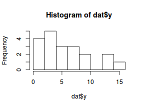
hist(dat$y)
boxplot(dat$y, horizontal=TRUE)
rug(jitter(dat$y), side=1)
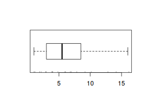
There is definitely signs of non-normality that would warrant Poisson models. The rug applied to the boxplots does not indicate a series degree of clumping and there appears to be few zero. Thus overdispersion is unlikely to be an issue.
Confirm linearity
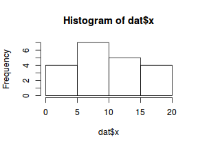
Lets now explore linearity by creating a histogram of the predictor variable ($x$) and a scatterplot of the relationship between the response ($y$) and the predictor ($x$)
hist(dat$x)
#now for the scatterplot
plot(y~x, dat, log="y")
with(dat, lines(lowess(y~x)))
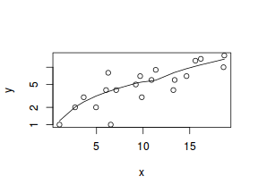
Conclusions: the predictor ($x$) does not display any skewness or other issues that might lead to non-linearity. The lowess smoother on the scatterplot does not display major deviations from a straight line and thus linearity is satisfied. Violations of linearity could be addressed by either:
- define a non-linear linear predictor (such as a polynomial, spline or other non-linear function)
- transform the scale of the predictor variables
Explore zero inflation
Although we have already established that there are few zeros in the data (and thus overdispersion is unlikely to be an issue), we can also explore this by comparing the number of zeros in the data to the number of zeros that would be expected from a Poisson distribution with a mean equal to the mean count of the data.
#proportion of 0's in the data
dat.tab<-table(dat$y==0)
dat.tab/sum(dat.tab)
FALSE
    1
#proportion of 0's expected from a Poisson distribution
mu <- mean(dat$y)
cnts <- rpois(1000, mu)
dat.tab <- table(cnts == 0)
dat.tab/sum(dat.tab)
FALSE  TRUE
0.997 0.003
0.003).
Model fitting or statistical analysis
JAGS
$$ \begin{align} Y_i&\sim{}P(\lambda) & (\text{response distribution})\\ log(\lambda_i)&=\eta_i & (\text{link function})\\ \eta_i&=\beta_0+\beta_1 X_i & (\text{linear predictor})\\ \beta_0, \beta_1&\sim{}\mathcal{N}(0,10000) & (\text{diffuse Bayesian prior})\\ \end{align} $$dat.list <- with(dat,list(Y=y, X=x,N=nrow(dat))) modelString=" model { for (i in 1:N) { Y[i] ~ dpois(lambda[i]) log(lambda[i]) <- beta0 + beta1*X[i] } beta0 ~ dnorm(0,1.0E-06) beta1 ~ dnorm(0,1.0E-06) } " writeLines(modelString,con='../downloads/BUGSscripts/tut11.5bS1.4.bug') library(R2jags) system.time( dat.P.jags <- jags(model='../downloads/BUGSscripts/tut11.5bS1.4.bug', data=dat.list, inits=NULL, param=c('beta0','beta1'), n.chain=3, n.iter=20000, n.thin=10, n.burnin=10000) )
Compiling model graph
   Resolving undeclared variables
   Allocating nodes
   Graph Size: 105

Initializing model
   user  system elapsed
  1.852   0.004   1.861
Xmat <- model.matrix(~x, dat)
nX <- ncol(Xmat)
dat.list1 <- with(dat,list(Y=y, X=Xmat,N=nrow(dat), nX=nX))
modelString="
model {
  for (i in 1:N) {
     Y[i] ~ dpois(lambda[i])
     eta[i] <- inprod(beta[], X[i,])
     log(lambda[i]) <- eta[i]
  }
  for (i in 1:nX) {
    beta[i] ~ dnorm(0,1.0E-06)
  }
}
"
writeLines(modelString,con='../downloads/BUGSscripts/tut11.5bS1.41.bug')
library(R2jags)
system.time(
dat.P.jags1 <- jags(model='../downloads/BUGSscripts/tut11.5bS1.41.bug', data=dat.list1, inits=NULL,
          param=c('beta'),
          n.chain=3,
          n.iter=20000, n.thin=10, n.burnin=10000)
  )
Compiling model graph
   Resolving undeclared variables
   Allocating nodes
   Graph Size: 127

Initializing model
   user  system elapsed
  1.836   0.004   1.844
print(dat.P.jags1)
Inference for Bugs model at "../downloads/BUGSscripts/tut11.5bS1.41.bug", fit using jags,
 3 chains, each with 20000 iterations (first 10000 discarded), n.thin = 10
 n.sims = 3000 iterations saved
         mu.vect sd.vect   2.5%    25%    50%    75%  97.5%  Rhat n.eff
beta[1]    0.546   0.256  0.019  0.384  0.552  0.719  1.018 1.002  1700
beta[2]    0.112   0.019  0.077  0.099  0.112  0.124  0.149 1.002  1800
deviance  88.428   4.999 86.376 86.891 87.680 89.036 93.531 1.001  3000

For each parameter, n.eff is a crude measure of effective sample size,
and Rhat is the potential scale reduction factor (at convergence, Rhat=1).

DIC info (using the rule, pD = var(deviance)/2)
pD = 12.5 and DIC = 100.9
DIC is an estimate of expected predictive error (lower deviance is better).
Or arguably better still, use a multivariate normal prior. If we have a $k$ regression parameters ($\beta_k$), then the multivariate normal priors are defined as: $$ \boldsymbol{\beta}\sim{}\mathcal{N_k}(\boldsymbol{\mu}, \mathbf{\Sigma}) $$ where $$\boldsymbol{\mu}=[E[\beta_1],E[\beta_2],...,E[\beta_k]] = \left(\begin{array}{c}0\\\vdots\\0\end{array}\right)$$ $$ \mathbf{\Sigma}=[Cov[\beta_i, \beta_j]] = \left(\begin{array}{ccc}1000^2&0&0\\0&\ddots&0\\0&0&1000^2\end{array} \right) $$ hence, along with the response and predictor matrix, we need to supply $\boldsymbol{\mu}$ (a vector of zeros) and $\boldsymbol{\Sigma}$ (a covariance matrix with $1000^2$ in the diagonals).
Xmat <- model.matrix(~x, dat)
nX <- ncol(Xmat)
dat.list2 <- with(dat,list(Y=y, X=Xmat,N=nrow(dat), mu=rep(0,nX),Sigma=diag(1.0E-06,nX)))
modelString="
model {
  for (i in 1:N) {
     Y[i] ~ dpois(lambda[i])
     eta[i] <- inprod(beta[], X[i,])
     log(lambda[i]) <- eta[i]
  }
  beta ~ dmnorm(mu[],Sigma[,])
}
"
writeLines(modelString,con='../downloads/BUGSscripts/tut11.5bS1.42.bug')
library(R2jags)
system.time(
dat.P.jags2 <- jags(model='../downloads/BUGSscripts/tut11.5bS1.42.bug', data=dat.list2, inits=NULL,
          param=c('beta'),
          n.chain=3,
          n.iter=20000, n.thin=10, n.burnin=10000)
  )
Compiling model graph
   Resolving undeclared variables
   Allocating nodes
   Graph Size: 130

Initializing model
   user  system elapsed
  0.460   0.000   0.463
print(dat.P.jags2)
Inference for Bugs model at "../downloads/BUGSscripts/tut11.5bS1.42.bug", fit using jags,
 3 chains, each with 20000 iterations (first 10000 discarded), n.thin = 10
 n.sims = 3000 iterations saved
         mu.vect sd.vect   2.5%    25%    50%    75%  97.5%  Rhat n.eff
beta[1]    0.561   0.241  0.084  0.405  0.571  0.724  1.034 1.002  1500
beta[2]    0.111   0.018  0.074  0.099  0.111  0.123  0.145 1.002  1300
deviance  88.184   1.850 86.372 86.854 87.596 88.898 92.951 1.007   900

For each parameter, n.eff is a crude measure of effective sample size,
and Rhat is the potential scale reduction factor (at convergence, Rhat=1).

DIC info (using the rule, pD = var(deviance)/2)
pD = 1.7 and DIC = 89.9
DIC is an estimate of expected predictive error (lower deviance is better).
BRMS
library(brms)
dat.brm <- brm(y~x, data=dat, family='poisson',
  prior = c(set_prior("normal(0,100)", class="b")),
  chains=3, iter=2000, warmup=1000, thin=2)
SAMPLING FOR MODEL 'poisson(log) brms-model' NOW (CHAIN 1).

Chain 1, Iteration:    1 / 2000 [  0%]  (Warmup)
Chain 1, Iteration:  200 / 2000 [ 10%]  (Warmup)
Chain 1, Iteration:  400 / 2000 [ 20%]  (Warmup)
Chain 1, Iteration:  600 / 2000 [ 30%]  (Warmup)
Chain 1, Iteration:  800 / 2000 [ 40%]  (Warmup)
Chain 1, Iteration: 1000 / 2000 [ 50%]  (Warmup)
Chain 1, Iteration: 1001 / 2000 [ 50%]  (Sampling)
Chain 1, Iteration: 1200 / 2000 [ 60%]  (Sampling)
Chain 1, Iteration: 1400 / 2000 [ 70%]  (Sampling)
Chain 1, Iteration: 1600 / 2000 [ 80%]  (Sampling)
Chain 1, Iteration: 1800 / 2000 [ 90%]  (Sampling)
Chain 1, Iteration: 2000 / 2000 [100%]  (Sampling)#
#  Elapsed Time: 0.03963 seconds (Warm-up)
#                0.03519 seconds (Sampling)
#                0.07482 seconds (Total)
#

SAMPLING FOR MODEL 'poisson(log) brms-model' NOW (CHAIN 2).

Chain 2, Iteration:    1 / 2000 [  0%]  (Warmup)
Chain 2, Iteration:  200 / 2000 [ 10%]  (Warmup)
Chain 2, Iteration:  400 / 2000 [ 20%]  (Warmup)
Chain 2, Iteration:  600 / 2000 [ 30%]  (Warmup)
Chain 2, Iteration:  800 / 2000 [ 40%]  (Warmup)
Chain 2, Iteration: 1000 / 2000 [ 50%]  (Warmup)
Chain 2, Iteration: 1001 / 2000 [ 50%]  (Sampling)
Chain 2, Iteration: 1200 / 2000 [ 60%]  (Sampling)
Chain 2, Iteration: 1400 / 2000 [ 70%]  (Sampling)
Chain 2, Iteration: 1600 / 2000 [ 80%]  (Sampling)
Chain 2, Iteration: 1800 / 2000 [ 90%]  (Sampling)
Chain 2, Iteration: 2000 / 2000 [100%]  (Sampling)#
#  Elapsed Time: 0.038022 seconds (Warm-up)
#                0.035344 seconds (Sampling)
#                0.073366 seconds (Total)
#

SAMPLING FOR MODEL 'poisson(log) brms-model' NOW (CHAIN 3).

Chain 3, Iteration:    1 / 2000 [  0%]  (Warmup)
Chain 3, Iteration:  200 / 2000 [ 10%]  (Warmup)
Chain 3, Iteration:  400 / 2000 [ 20%]  (Warmup)
Chain 3, Iteration:  600 / 2000 [ 30%]  (Warmup)
Chain 3, Iteration:  800 / 2000 [ 40%]  (Warmup)
Chain 3, Iteration: 1000 / 2000 [ 50%]  (Warmup)
Chain 3, Iteration: 1001 / 2000 [ 50%]  (Sampling)
Chain 3, Iteration: 1200 / 2000 [ 60%]  (Sampling)
Chain 3, Iteration: 1400 / 2000 [ 70%]  (Sampling)
Chain 3, Iteration: 1600 / 2000 [ 80%]  (Sampling)
Chain 3, Iteration: 1800 / 2000 [ 90%]  (Sampling)
Chain 3, Iteration: 2000 / 2000 [100%]  (Sampling)#
#  Elapsed Time: 0.038597 seconds (Warm-up)
#                0.037356 seconds (Sampling)
#                0.075953 seconds (Total)
#
Chain mixing and Model validation
Prior to exploring the model parameters, it is prudent to confirm that the model did indeed fit the assumptions and was an appropriate fit to the data as well as that the MCMC sampling chain was adequately mixed and the retained samples independent.
Whilst I will only demonstrate this for the logit model, the procedure would be identical for exploring the probit and clog-log models.
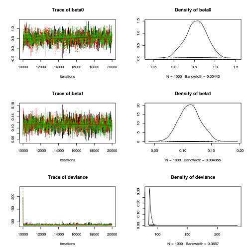
- We will start by exploring the mixing of the MCMC chains via traceplots.
plot(as.mcmc(dat.P.jags))
library(gridExtra)
grid.arrange(stan_trace(dat.brm$fit, ncol=1),
             stan_dens(dat.brm$fit, separate_chains=TRUE,ncol=1),
             ncol=2)
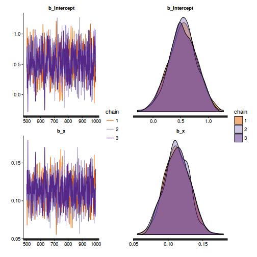
The chains appear well mixed and stable
- Next we will explore correlation amongst MCMC samples.
autocorr.diag(as.mcmc(dat.P.jags))
             beta0    beta1  deviance
Lag 0    1.0000000  1.00000  1.000000
Lag 10   0.1553164  0.11400  0.009912
Lag 50   0.0228548  0.01439  0.004464
Lag 100 -0.0008548 -0.01320  0.001207
Lag 500 -0.0339699 -0.02674 -0.007545
The level of auto-correlation at the nominated lag of 10 is higher than we would generally like. It is worth increasing the thinning rate from 10 to 50. Obviously, to support this higher thinning rate, we would also increase the number of iterations.
library(R2jags)
dat.P.jags <- jags(data=dat.list,model.file='../downloads/BUGSscripts/tut11.5bS1.4.bug',
                   param=c('beta0','beta1'),
                   n.chains=3, n.iter=100000, n.burnin=20000, n.thin=50)
Compiling model graph
   Resolving undeclared variables
   Allocating nodes
   Graph Size: 105

Initializing model
print(dat.P.jags)
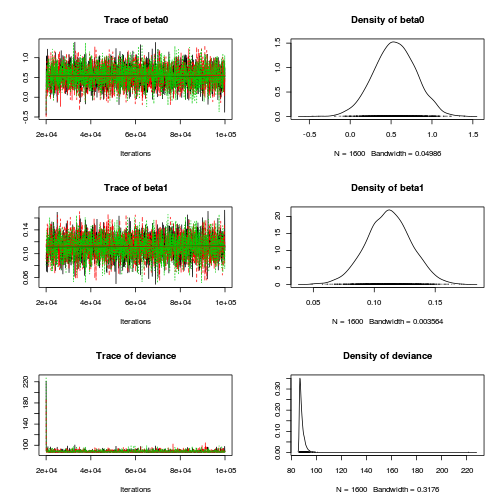
Inference for Bugs model at "../downloads/BUGSscripts/tut11.5bS1.4.bug", fit using jags, 3 chains, each with 1e+05 iterations (first 20000 discarded), n.thin = 50 n.sims = 4800 iterations saved mu.vect sd.vect 2.5% 25% 50% 75% 97.5% Rhat n.eff beta0 0.545 0.257 0.040 0.375 0.545 0.718 1.039 1.001 4800 beta1 0.112 0.019 0.075 0.100 0.112 0.124 0.148 1.001 4800 deviance 88.379 3.712 86.368 86.871 87.664 89.058 93.778 1.002 4800 For each parameter, n.eff is a crude measure of effective sample size, and Rhat is the potential scale reduction factor (at convergence, Rhat=1). DIC info (using the rule, pD = var(deviance)/2) pD = 6.9 and DIC = 95.3 DIC is an estimate of expected predictive error (lower deviance is better).plot(as.mcmc(dat.P.jags))
autocorr.diag(as.mcmc(dat.P.jags))
             beta0    beta1 deviance
Lag 0    1.0000000 1.000000 1.000000
Lag 50   0.0100259 0.009642 0.003845
Lag 250  0.0133849 0.010277 0.001847
Lag 500  0.0056560 0.003987 0.001649
Lag 2500 0.0006608 0.003896 0.007031
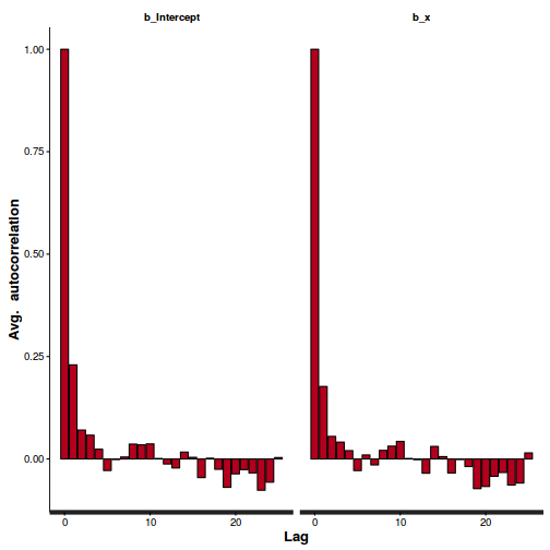
Conclusions: the samples are now less auto-correlated and the chains are also arguably mixed a little better.
stan_ac(dat.brm$fit)
- Explore the step size characteristics (STAN only)
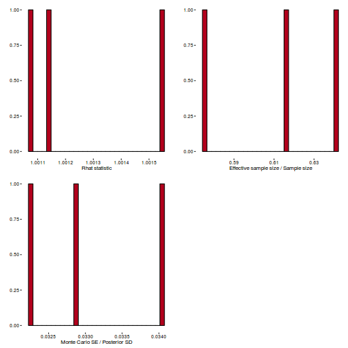
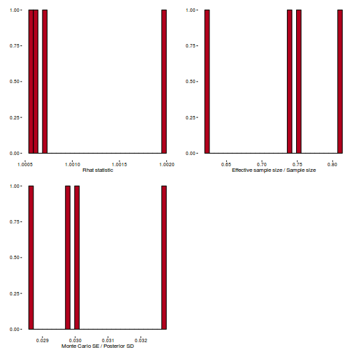
Conclusions: acceptance ratio is very good, the lot posterior is relatively robust to step size and tree depth, rhat values are all below 1.05, the effective sample size is always above 0.5 and the ratio of MCMC error to posterior sd is very small.
summary(do.call(rbind, args = get_sampler_params(dat.brm$fit, inc_warmup = FALSE)), digits = 2)
 accept_stat__    stepsize__    treedepth__   n_leapfrog__ n_divergent__
 Min.   :0.24   Min.   :0.64   Min.   :1.0   Min.   :1.0   Min.   :0
 1st Qu.:0.88   1st Qu.:0.64   1st Qu.:2.0   1st Qu.:3.0   1st Qu.:0
 Median :0.96   Median :0.72   Median :2.0   Median :3.0   Median :0
 Mean   :0.92   Mean   :0.70   Mean   :2.1   Mean   :3.7   Mean   :0
 3rd Qu.:1.00   3rd Qu.:0.73   3rd Qu.:3.0   3rd Qu.:5.0   3rd Qu.:0
 Max.   :1.00   Max.   :0.73   Max.   :3.0   Max.   :7.0   Max.   :0
stan_diag(dat.brm$fit)
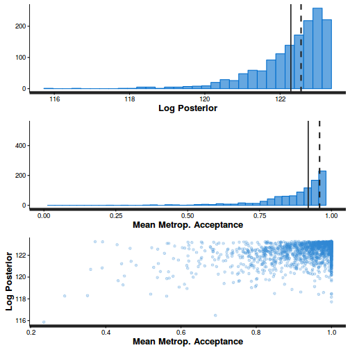
stan_diag(dat.brm$fit, information = "stepsize")
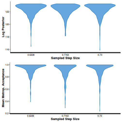
stan_diag(dat.brm$fit, information = "treedepth")
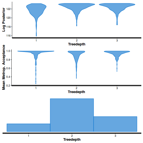
stan_diag(dat.brm$fit, information = "divergence")
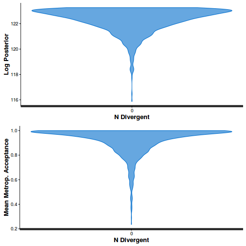
library(gridExtra)
grid.arrange(stan_rhat(dat.brm$fit) + theme_classic(8),
             stan_ess(dat.brm$fit) + theme_classic(8),
             stan_mcse(dat.brm$fit) + theme_classic(8),
             ncol = 2)
- One very important model validation procedure is to examine a plot of residuals against predicted or fitted values (the residual plot).
Ideally, residual plots should show a random scatter of points without outliers.
That is, there should be no patterns in the residuals. Patterns suggest inappropriate linear predictor (or scale) and/or inappropriate
residual distribution/link function.
The residuals used in such plots should be standardized (particularly if the model incorporated any variance-covariance structures - such as an autoregressive correlation structure)
Pearsons's residuals standardize residuals by division with the square-root of the variance.
We can generate Pearson's residuals within the JAGS model.
Alternatively, we could use the parameters to generate the residuals outside of JAGS.
Pearson's residuals are calculated according to:
$$
\varepsilon = \frac{y_i - \mu}{\sqrt{var(y)}}
$$
where $\mu$ is the expected value of $Y$ ($=\lambda$ for Poisson) and $var(y)$ is the variance of $Y$ ($=\lambda$ for Poisson).
#extract the samples for the two model parameters
coefs <- dat.P.jags$BUGSoutput$sims.matrix[,1:2]
Xmat <- model.matrix(~x, data=dat)
#expected values on a log scale
eta<-coefs %*% t(Xmat)
#expected value on response scale
lambda <- exp(eta)
#Expected value and variance are both equal to lambda
expY <- varY <- lambda
#sweep across rows and then divide by lambda
Resid <- -1*sweep(expY,2,dat$y,'-')/sqrt(varY)
#plot residuals vs expected values
plot(apply(Resid,2,mean)~apply(eta,2,mean))

#Calculate residuals
Resid.brm <- residuals(dat.brm, type='pearson')
Fitted.brm <- fitted(dat.brm, scale='linear')
ggplot(data=NULL, aes(y=Resid.brm[,'Estimate'], x=Fitted.brm[,'Estimate'])) + geom_point()
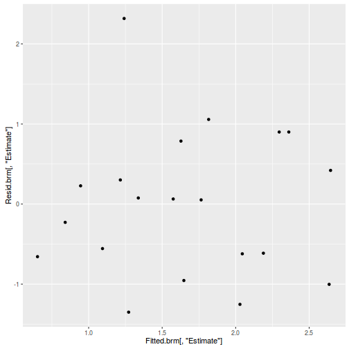
There is one residual that is substantially larger in magnitude than all the others. However, there are no other patterns in the residuals.
- Now we will compare the sum of squared residuals to the sum of squares residuals that would be expected from a Poisson distribution
matching that estimated by the model. Essentially this is estimating how well the Poisson distribution, the log-link function and the linear model
approximates the observed data.
SSres<-apply(Resid^2,1,sum)

set.seed(2)
#generate a matrix of draws from a poisson distribution
# the matrix is the same dimensions as lambda and uses the probabilities of lambda
YNew <- matrix(rpois(length(lambda),lambda=lambda),nrow=nrow(lambda))

Resid1<-(lambda - YNew)/sqrt(lambda)
SSres.sim<-apply(Resid1^2,1,sum)
mean(SSres.sim>SSres)
[1] 0.484375
dat.list1 <- with(dat,list(Y=y, X=x,N=nrow(dat)))
modelString="
model {
  for (i in 1:N) {
    #likelihood function
    Y[i] ~ dpois(lambda[i])
    eta[i] <- beta0+beta1*X[i] #linear predictor
    log(lambda[i]) <- eta[i]   #link function

    #E(Y) and var(Y)
    expY[i] <- lambda[i]
    varY[i] <- lambda[i]

    # Calculate RSS
    Resid[i] <- (Y[i] - expY[i])/sqrt(varY[i])
    RSS[i] <- pow(Resid[i],2)

    #Simulate data from a Poisson distribution
    Y1[i] ~ dpois(lambda[i])
    #Calculate RSS for simulated data
    Resid1[i] <- (Y1[i] - expY[i])/sqrt(varY[i])
    RSS1[i] <-pow(Resid1[i],2)
  }
  #Priors
  beta0 ~ dnorm(0,1.0E-06)
  beta1 ~ dnorm(0,1.0E-06)
  #Bayesian P-value
  Pvalue <- mean(sum(RSS1)>sum(RSS))
}
"
writeLines(modelString,con='../downloads/BUGSscripts/tut11.5bS6.41.bug')
library(R2jags)
system.time(
dat.P.jags1 <- jags(model='../downloads/BUGSscripts/tut11.5bS6.41.bug', data=dat.list1, inits=NULL,
          param=c('beta0','beta1','Pvalue'),
          n.chain=3,
          n.iter=100000, n.thin=50, n.burnin=20000)
  )
Compiling model graph
   Resolving undeclared variables
   Allocating nodes
   Graph Size: 272

Initializing model
   user  system elapsed
 16.189   0.004  16.209
print(dat.P.jags1)
Inference for Bugs model at "../downloads/BUGSscripts/tut11.5bS6.41.bug", fit using jags, 3 chains, each with 1e+05 iterations (first 20000 discarded), n.thin = 50 n.sims = 4800 iterations saved mu.vect sd.vect 2.5% 25% 50% 75% 97.5% Rhat n.eff Pvalue 0.481 0.500 0.000 0.000 0.000 1.000 1.00 1.001 4800 beta0 0.544 0.261 0.017 0.374 0.550 0.720 1.04 1.002 1200 beta1 0.112 0.019 0.075 0.099 0.112 0.125 0.15 1.002 1600 deviance 88.466 3.891 86.372 86.931 87.758 89.180 93.91 1.001 4800 For each parameter, n.eff is a crude measure of effective sample size, and Rhat is the potential scale reduction factor (at convergence, Rhat=1). DIC info (using the rule, pD = var(deviance)/2) pD = 7.6 and DIC = 96.0 DIC is an estimate of expected predictive error (lower deviance is better).Resid.brm <- residuals(dat.brm, type='pearson', summary=FALSE) SSres.brm <- apply(Resid.brm^2,1,sum) lambda.brm = fitted(dat.brm, scale='response', summary=FALSE) YNew.brm <- matrix(rpois(length(lambda.brm), lambda=lambda.brm),nrow=nrow(lambda.brm)) Resid1.brm<-(lambda.brm - YNew.brm)/sqrt(lambda.brm) SSres.sim.brm<-apply(Resid1.brm^2,1,sum) mean(SSres.sim.brm>SSres.brm)
[1] 0.6026667
Conclusions: the Bayesian p-value is approximately 0.5, suggesting that there is a good fit of the model to the data.
- Unfortunately, unlike with linear models (Gaussian family), the expected distribution of data (residuals) varies
over the range of fitted values for numerous (often competing) ways that make diagnosing (and attributing causes
thereof) miss-specified generalized linear models from standard residual plots very difficult. The use of standardized
(Pearson) residuals or deviance residuals can partly address this issue, yet they still do not offer completely
consistent diagnoses across all issues (miss-specified model, over-dispersion, zero-inflation).
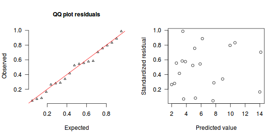
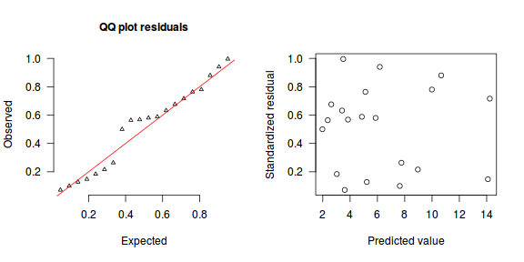
An alternative approach is to use simulated data from the model posteriors to calculate an empirical cumulative density function from which residuals are are generated as values corresponding to the observed data along the density function.
The trend (black symbols) in the qq-plot does not appear to be overly non-linear (matching the ideal red line well), suggesting that the model is not overdispersed. The spread of standardized (simulated) residuals in the residual plot do not appear overly non-uniform. That is there is not trend in the residuals. Furthermore, there is not a concentration of points close to 1 or 0 (which would imply overdispersion).#extract the samples for the two model parameters coefs <- dat.P.jags$BUGSoutput$sims.matrix[,1:2] Xmat <- model.matrix(~x, data=dat) #expected values on a log scale eta<-coefs %*% t(Xmat) #expected value on response scale lambda <- exp(eta) simRes <- function(lambda, data,n=250, plot=T, family='poisson') { require(gap) N = nrow(data) sim = switch(family, 'poisson' = matrix(rpois(n*N,apply(lambda,2,mean)),ncol=N, byrow=TRUE) ) a = apply(sim + runif(n,-0.5,0.5),2,ecdf) resid<-NULL for (i in 1:nrow(data)) resid<-c(resid,a[[i]](data$y[i] + runif(1 ,-0.5,0.5))) if (plot==T) { par(mfrow=c(1,2)) gap::qqunif(resid,pch = 2, bty = "n", logscale = F, col = "black", cex = 0.6, main = "QQ plot residuals", cex.main = 1, las=1) plot(resid~apply(lambda,2,mean), xlab='Predicted value', ylab='Standardized residual', las=1) } resid } simRes(lambda,dat, family='poisson')
[1] 0.264 0.280 0.556 0.416 0.584 0.988 0.068 0.576 0.524 0.756 0.080 0.544 0.888 0.044 0.288 0.340 0.796 0.832 0.164 0.704
lambda.brm = fitted(dat.brm, scale='response', summary=FALSE)

simRes <- function(lambda, data,n=250, plot=T, family='poisson') {
 require(gap)
 N = nrow(data)
 sim = switch(family,
    'poisson' = matrix(rpois(n*N,apply(lambda,2,mean)),ncol=N, byrow=TRUE)
 )
 a = apply(sim + runif(n,-0.5,0.5),2,ecdf)
 resid<-NULL
 for (i in 1:nrow(data)) resid<-c(resid,a[[i]](data$y[i] + runif(1 ,-0.5,0.5)))
 if (plot==T) {
   par(mfrow=c(1,2))
   gap::qqunif(resid,pch = 2, bty = "n",
   logscale = F, col = "black", cex = 0.6, main = "QQ plot residuals",
   cex.main = 1, las=1)
   plot(resid~apply(lambda,2,mean), xlab='Predicted value', ylab='Standardized residual', las=1)
 }
 resid
}

simRes(lambda.brm, dat, family='poisson')
[1] 0.500 0.564 0.676 0.184 0.632 0.996 0.072 0.568 0.588 0.764 0.128 0.580 0.940 0.100 0.264 0.216 0.780 0.880 0.148 0.716
-
Recall that the Poisson regression model assumes that variance=mean ($var=\mu\phi$ where $\phi=1$) and thus dispersion ($\phi=\frac{var}{\mu}=1$).
However, we can also calculate approximately what the dispersion factor would be by using sum square of the residuals as a measure of variance and the model
residual degrees of freedom as a measure of the mean (since the expected value of a Poisson distribution is the same as its degrees of freedom).
$$\phi=\frac{RSS}{df}$$ where $df=n-k$ and $k$ is the number of estimated model coefficients.
Resid <- -1*sweep(lambda,2,dat$y,'-')/sqrt(lambda)
RSS<-apply(Resid^2,1,sum)
(df<-nrow(dat)-ncol(coefs))
[1] 18
Disp <- RSS/df
data.frame(Median=median(Disp), Mean=mean(Disp), HPDinterval(as.mcmc(Disp)),
           HPDinterval(as.mcmc(Disp),p=0.5))
       Median     Mean     lower    upper   lower.1  upper.1
var1 1.044197 1.109181 0.9299409 1.452832 0.9299853 1.044238
dat.list <- with(dat,list(Y=y, X=x,N=nrow(dat)))
modelString="
model {
  for (i in 1:N) {
     Y[i] ~ dpois(lambda[i])
     eta[i] <- beta0 + beta1*X[i]
     log(lambda[i]) <- eta[i]
     expY[i] <- lambda[i]
     varY[i] <- lambda[i]
	 Resid[i] <- (Y[i] - expY[i])/sqrt(varY[i])
  }
  beta0 ~ dnorm(0,1.0E-06)
  beta1 ~ dnorm(0,1.0E-06)
  RSS <- sum(pow(Resid,2))
  df <- N-2
  phi <- RSS/df
}
"
writeLines(modelString,con='tut11.5bS1.40.bug')
library(R2jags)
system.time(
dat.P.jags <- jags(model='tut11.5bS1.40.bug', data=dat.list, inits=NULL,
          param=c('beta0','beta1','phi'),
          n.chain=3,
          n.iter=100000, n.thin=50, n.burnin=20000)
  )
Compiling model graph
   Resolving undeclared variables
   Allocating nodes
   Graph Size: 171

Initializing model
   user  system elapsed
 14.865   0.004  14.886
print(dat.P.jags)
Inference for Bugs model at "tut11.5bS1.40.bug", fit using jags, 3 chains, each with 1e+05 iterations (first 20000 discarded), n.thin = 50 n.sims = 4800 iterations saved mu.vect sd.vect 2.5% 25% 50% 75% 97.5% Rhat n.eff beta0 0.542 0.258 0.013 0.37 0.544 0.716 1.042 1.001 4800 beta1 0.112 0.019 0.075 0.10 0.112 0.125 0.149 1.001 4800 phi 1.112 0.400 0.934 0.98 1.052 1.173 1.570 1.001 4800 deviance 88.433 3.859 86.373 86.89 87.727 89.159 93.839 1.001 4800 For each parameter, n.eff is a crude measure of effective sample size, and Rhat is the potential scale reduction factor (at convergence, Rhat=1). DIC info (using the rule, pD = var(deviance)/2) pD = 7.4 and DIC = 95.9 DIC is an estimate of expected predictive error (lower deviance is better).Resid.brm <- residuals(dat.brm, type='pearson', summary=FALSE) SSres.brm <- apply(Resid.brm^2,1,sum) (df <- nrow(dat) - nrow(coef(dat.brm)))
[1] 18
Disp <- SSres.brm/df
data.frame(Median=median(Disp), Mean=mean(Disp), HPDinterval(as.mcmc(Disp)),
           HPDinterval(as.mcmc(Disp)))
        Median      Mean     lower    upper   lower.1  upper.1
var1 0.9666143 0.9944079 0.8964392 1.168199 0.8964392 1.168199
The dispersion statistic $\phi$ is close to 1 and thus there is no evidence that the data were overdispersed. The Poisson distribution was therefore appropriate.
Exploring the model parameters, test hypotheses
If there was any evidence that the assumptions had been violated or the model was not an appropriate fit, then we would need to reconsider the model and start the process again. In this case, there is no evidence that the test will be unreliable so we can proceed to explore the test statistics.
print(dat.P.jags)
Inference for Bugs model at "tut11.5bS1.40.bug", fit using jags,
 3 chains, each with 1e+05 iterations (first 20000 discarded), n.thin = 50
 n.sims = 4800 iterations saved
         mu.vect sd.vect   2.5%   25%    50%    75%  97.5%  Rhat n.eff
beta0      0.542   0.258  0.013  0.37  0.544  0.716  1.042 1.001  4800
beta1      0.112   0.019  0.075  0.10  0.112  0.125  0.149 1.001  4800
phi        1.112   0.400  0.934  0.98  1.052  1.173  1.570 1.001  4800
deviance  88.433   3.859 86.373 86.89 87.727 89.159 93.839 1.001  4800

For each parameter, n.eff is a crude measure of effective sample size,
and Rhat is the potential scale reduction factor (at convergence, Rhat=1).

DIC info (using the rule, pD = var(deviance)/2)
pD = 7.4 and DIC = 95.9
DIC is an estimate of expected predictive error (lower deviance is better).
library(plyr)
adply(dat.P.jags$BUGSoutput$sims.matrix[,1:2], 2, function(x) {
  data.frame(Median=median(x), Mean=mean(x), HPDinterval(as.mcmc(x)), HPDinterval(as.mcmc(x),p=0.5))
})
     X1 Median   Mean   lower  upper lower.1 upper.1
1 beta0 0.5445 0.5423 0.02752 1.0480  0.3617  0.7056
2 beta1 0.1123 0.1122 0.07599 0.1491  0.1001  0.1251
Actually, many find it more palatable to express the estimates in the original scale of the observations rather than on a log scale.
library(plyr)
adply(exp(dat.P.jags$BUGSoutput$sims.matrix[,1:2]), 2, function(x) {
  data.frame(Median=median(x), Mean=mean(x), HPDinterval(as.mcmc(x)), HPDinterval(as.mcmc(x),p=0.5))
})
     X1 Median  Mean  lower upper lower.1 upper.1
1 beta0  1.724 1.778 0.9645 2.709   1.342   1.915
2 beta1  1.119 1.119 1.0790 1.161   1.105   1.133
Conclusions:
We would reject the null hypothesis of no effect of $x$ on $y$.
An increase in x is associated with a significant linear increase (positive slope) in the abundance of $y$.
Every 1 unit increase in $x$ results in a log 0.1123415 unit increase in $y$.
We usually express this in terms of abundance rather than log abundance, so
every 1 unit increase in $x$ results in a ($e^{ 0.1123415 } = 1.1188949 $)
1.1188949 unit increase in the abundance of $y$.
summary(dat.brm)
 Family: poisson (log)
Formula: y ~ x
   Data: dat (Number of observations: 20)
Samples: 3 chains, each with iter = 2000; warmup = 1000; thin = 2;
         total post-warmup samples = 1500
   WAIC: Not computed

Fixed Effects:
          Estimate Est.Error l-95% CI u-95% CI Eff.Sample Rhat
Intercept     0.54      0.25     0.04     1.01        864    1
x             0.11      0.02     0.08     0.15        962    1

Samples were drawn using sampling(NUTS). For each parameter, Eff.Sample
is a crude measure of effective sample size, and Rhat is the potential
scale reduction factor on split chains (at convergence, Rhat = 1).
exp(coef(dat.brm))
              mean
Intercept 1.710068
x         1.119290
coefs.brm <- as.matrix(as.data.frame(rstan:::extract(dat.brm$fit)))
coefs.brm <- coefs.brm[,grep('b', colnames(coefs.brm))]
plyr:::adply(exp(coefs.brm), 2, function(x) {
  data.frame(Mean=mean(x), median=median(x), HPDinterval(as.mcmc(x)))
  })
           X1     Mean   median    lower    upper
1 b_Intercept 1.763680 1.710650 0.950453 2.630181
2         b_x 1.119476 1.118679 1.082259 1.161513
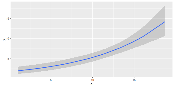
marginal_effects(dat.brm)
Further explorations of the trends
A measure of the strength of the relationship can be obtained according to: $$R^2 = 1 - \frac{RSS_{model}}{RSS_{null}}$$
Xmat <- model.matrix(~x, data=dat)
#expected values on a log scale
eta<-coefs %*% t(Xmat)
#expected value on response scale
lambda <- exp(eta)
#calculate the raw SS residuals
SSres <- apply((-1*(sweep(lambda,2,dat$y,'-')))^2,1,sum)
SSres.null <- sum((dat$y - mean(dat$y))^2)
#OR
SSres.null <- crossprod(dat$y - mean(dat$y))
#calculate the model r2
1-mean(SSres)/SSres.null
       [,1]
[1,] 0.6572
Conclusions: 65.72% of the variation in $y$ abundance can be explained by its relationship with $x$.
dat.list <- with(dat,list(Y=y, X=x,N=nrow(dat)))
modelString="
model {
  for (i in 1:N) {
     Y[i] ~ dpois(lambda[i])
     eta[i] <- beta0 + beta1*X[i]
     log(lambda[i]) <- eta[i]
     res[i] <- Y[i] - lambda[i]
     resnull[i] <- Y[i] - meanY
  }
  meanY <- mean(Y)
  beta0 ~ dnorm(0,1.0E-06)
  beta1 ~ dnorm(0,1.0E-06)
  RSS <- sum(res^2)
  RSSnull <- sum(resnull^2)
  r2 <- 1-RSS/RSSnull
}
"
writeLines(modelString,con='tut11.5bS1.40.bug')
library(R2jags)
system.time(
dat.P.jags <- jags(model='tut11.5bS1.40.bug', data=dat.list, inits=NULL,
          param=c('beta0','beta1','r2'),
          n.chain=3,
          n.iter=100000, n.thin=50, n.burnin=20000)
  )
Compiling model graph
   Resolving undeclared variables
   Allocating nodes
   Graph Size: 150

Initializing model
   user  system elapsed
 14.909   0.008  14.933
print(dat.P.jags)
Inference for Bugs model at "tut11.5bS1.40.bug", fit using jags,
 3 chains, each with 1e+05 iterations (first 20000 discarded), n.thin = 50
 n.sims = 4800 iterations saved
         mu.vect sd.vect   2.5%    25%    50%    75%  97.5%  Rhat n.eff
beta0      0.550   0.253  0.052  0.384  0.554  0.723  1.028 1.001  4800
beta1      0.112   0.019  0.076  0.099  0.112  0.124  0.149 1.001  4800
r2         0.655   0.066  0.509  0.640  0.673  0.691  0.701 1.001  4800
deviance  88.418   4.483 86.372 86.885 87.718 89.117 93.725 1.003  4800

For each parameter, n.eff is a crude measure of effective sample size,
and Rhat is the potential scale reduction factor (at convergence, Rhat=1).

DIC info (using the rule, pD = var(deviance)/2)
pD = 10.1 and DIC = 98.5
DIC is an estimate of expected predictive error (lower deviance is better).
## calculate the expected values on the response scale
lambda.brm = fitted(dat.brm, scale='response', summary=FALSE)
## calculate the raw SSresid
SSres.brm <- apply((-1*(sweep(lambda.brm,2,dat$y,'-')))^2,1,sum)
SSres.null <- sum((dat$y - mean(dat$y))^2)
#OR
SSres.null <- crossprod(dat$y - mean(dat$y))
#calculate the model r2
1-mean(SSres.brm)/SSres.null
          [,1]
[1,] 0.6570747
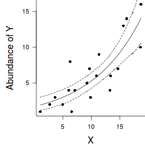
Finally, we will create a summary plot.
par(mar = c(4, 5, 0, 0))
plot(y ~ x, data = dat, type = "n", ann = F, axes = F)
points(y ~ x, data = dat, pch = 16)
xs <- seq(min(dat$x,na.rm=TRUE),max(dat$x,na.rm=TRUE), l = 1000)
Xmat <- model.matrix(~xs)
eta<-coefs %*% t(Xmat)
ys <- exp(eta)
library(plyr)
library(coda)
data.tab <- adply(ys,2,function(x) {
  data.frame(Median=median(x), HPDinterval(as.mcmc(x)))
})
data.tab <- cbind(x=xs,data.tab)
points(Median ~ x, data=data.tab,col = "black", type = "l")
lines(lower ~ x, data=data.tab,col = "black", type = "l", lty = 2)
lines(upper ~ x, data=data.tab,col = "black", type = "l", lty = 2)

axis(1)
mtext("X", 1, cex = 1.5, line = 3)
axis(2, las = 2)
mtext("Abundance of Y", 2, cex = 1.5, line = 3)
box(bty = "l")
newdata = data.frame(x=seq(min(dat$x), max(dat$x), len=100))
Xmat = model.matrix(~x, data=newdata)
coefs <- as.matrix(as.data.frame(rstan:::extract(dat.brm$fit)))
coefs <- coefs[,grep('b', colnames(coefs))]
fit = exp(coefs %*% t(Xmat))
newdata = cbind(newdata,
                plyr:::adply(fit, 2, function(x) {
                                  data.frame(Mean=mean(x), Median=median(x),
                                             HPDinterval(as.mcmc(x)))
                                })
)

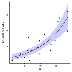
ggplot(newdata, aes(y=Mean, x=x)) +
  geom_point(data=dat, aes(y=y)) +
  geom_ribbon(aes(ymin=lower, ymax=upper), fill='blue',alpha=0.2) +
  geom_line() +
  scale_x_continuous('X') +
  scale_y_continuous('Abundance of Y') +
  theme_classic() +
  theme(axis.line.x=element_line(),axis.line.y=element_line())
Defining full log-likelihood function
Now lets try it by specifying log-likelihood and the zero trick. When applying this trick, we need to manually calculate the deviance as the inbuilt deviance will be based on the log-likelihood of estimating the zeros (as part of the zero trick) rather than the deviance of the intended model..
The one advantage of the zero trick is that the Deviance and thus DIC, AIC provided by R2jags will be incorrect. Hence, they too need to be manually defined within jags. I suspect that the AIC calculation I have used is incorrect...
Xmat <- model.matrix(~x, dat)
nX <- ncol(Xmat)
dat.list2 <- with(dat,list(Y=y, X=Xmat,N=nrow(dat), mu=rep(0,nX),
                  Sigma=diag(1.0E-06,nX), zeros=rep(0,nrow(dat)), C=10000))
modelString="
model {
  for (i in 1:N) {
     zeros[i] ~ dpois(zeros.lambda[i])
     zeros.lambda[i] <- -ll[i] + C
     ll[i] <- Y[i]*log(lambda[i]) - lambda[i] - loggam(Y[i]+1)
     eta[i] <- inprod(beta[], X[i,])
     log(lambda[i]) <- eta[i]
    llm[i] <- Y[i]*log(meanlambda) - meanlambda - loggam(Y[i]+1)
  }
  meanlambda <- mean(lambda)
  beta ~ dmnorm(mu[],Sigma[,])
  dev <- sum(-2*ll)
  pD <- mean(dev)-sum(-2*llm)
  AIC <- min(dev+(2*pD))
}
"
writeLines(modelString,con='../downloads/BUGSscripts/tut11.5bS1.42.bug')
library(R2jags)
system.time(
dat.P.jags3 <- jags(model='../downloads/BUGSscripts/tut11.5bS1.42.bug', data=dat.list2, inits=NULL,
          param=c('beta','dev','AIC'),
          n.chain=3,
          n.iter=50000, n.thin=50, n.burnin=10000)
  )
Compiling model graph
   Resolving undeclared variables
   Allocating nodes
   Graph Size: 353

Initializing model
   user  system elapsed
  1.936   0.004   1.942
print(dat.P.jags3)
Inference for Bugs model at "../downloads/BUGSscripts/tut11.5bS1.42.bug", fit using jags,
 3 chains, each with 50000 iterations (first 10000 discarded), n.thin = 50
 n.sims = 2400 iterations saved
           mu.vect sd.vect      2.5%       25%       50%       75%     97.5%  Rhat n.eff
AIC      1.328e+01   4.076 9.634e+00 1.050e+01 1.200e+01 1.458e+01 2.438e+01 1.001  2400
beta[1]  5.510e-01   0.245 6.200e-02 3.860e-01 5.540e-01 7.160e-01 1.008e+00 1.000  2400
beta[2]  1.120e-01   0.018 7.800e-02 9.900e-02 1.120e-01 1.240e-01 1.470e-01 1.001  2400
dev      8.821e+01   1.868 8.637e+01 8.686e+01 8.764e+01 8.897e+01 9.294e+01 1.002  2400
deviance 4.001e+05   1.868 4.001e+05 4.001e+05 4.001e+05 4.001e+05 4.001e+05 1.000     1

For each parameter, n.eff is a crude measure of effective sample size,
and Rhat is the potential scale reduction factor (at convergence, Rhat=1).

DIC info (using the rule, pD = var(deviance)/2)
pD = 1.7 and DIC = 400090.0
DIC is an estimate of expected predictive error (lower deviance is better).
Negative binomial
The following equations are provided since in Bayesian modelling, it is occasionally necessary to directly define the log-likelihood calculations (particularly for zero-inflated models and other mixture models). Feel free initially gloss over these equations until such time when your models require them ;)
| prob, size | alpha, beta (gamma-poisson) |
|---|---|
| $$ f(y|r,p)=\frac{\Gamma(y+r)}{\Gamma(r)\Gamma(y+1)}p^r(1-p)^y $$ where $p$ is the probability of $y$ successes until $r$ failures. If, we make $p=\frac{size}{size+\mu}$, then we can define the function in terms of $\mu$ $$ f(y|r,\mu)=\frac{\Gamma(y+r)}{\Gamma(r)\Gamma(y+1)}\left(\frac{r}{\mu+r}\right)^r\left(1-\frac{r}{\mu+r}\right)^y $$ where $p$ is the probability of $y$ successes until $r$ failures. $$\mu = \frac{r(1-p)}{p}\\ E(Y)=\mu, Var(Y)=\mu+\frac{\mu^2}{r} $$ | $$ f(y \mid \alpha, \beta) = \frac{\beta^{\alpha}y^{\alpha-1}e^{-\beta y}}{\Gamma(\alpha)} $$ where $$ \begin{align} l(\lambda;y)=&\sum\limits^n_{i=1} log\Gamma(y_i + \alpha) - log\Gamma(y_i+1) - log\Gamma(\alpha) + \\ & \alpha(log(\beta_i) - log(\beta_i+1)) - y_i.log(\beta_i+1) \end{align} $$ |
Scenario and Data
Lets say we wanted to model the abundance of an item ($y$) against a continuous predictor ($x$). As this section is mainly about the generation of artificial data (and not specifically about what to do with the data), understanding the actual details are optional and can be safely skipped. Consequently, I have folded (toggled) this section away.
- the sample size = 20
- the continuous $x$ variable is a random uniform spread of measurements between 1 and 20
- the rate of change in log $y$ per unit of $x$ (slope) = 0.1.
- the value of $x$ when log$y$ equals 0 (when $y$=1)
- to generate the values of $y$ expected at each $x$ value, we evaluate the linear predictor (created by calculating the outer product of the model matrix and the regression parameters). These expected values are then transformed into a scale mapped by (0,$\infty$) by using the log function $e^{linear~predictor}$
- finally, we generate $y$ values by using the expected $y$ values ($\lambda$) as probabilities when drawing random numbers from a Poisson distribution. This step adds random noise to the expected $y$ values and returns only 0's and positive integers.
set.seed(37) #16 #35
#The number of samples
n.x <- 20
#Create x values that at uniformly distributed throughout the rate of 1 to 20
x <- sort(runif(n = n.x, min = 1, max =20))
mm <- model.matrix(~x)
intercept <- 0.6
slope=0.1
#The linear predictor
linpred <- mm %*% c(intercept,slope)
#Predicted y values
lambda <- exp(linpred)
#Add some noise and make binomial
y <- rnbinom(n=n.x, mu=lambda, size=1)
dat.nb <- data.frame(y,x)
Exploratory data analysis and initial assumption checking
- All of the observations are independent - this must be addressed at the design and collection stages
- The response variable (and thus the residuals) should be matched by an appropriate distribution (in the case of positive integers response - a Poisson is appropriate).
- All observations are equally influential in determining the trends - or at least no observations are overly influential. This is most effectively diagnosed via residuals and other influence indices and is very difficult to diagnose prior to analysis
- the relationship between the linear predictor (right hand side of the regression formula) and the link function should be linear. A scatterplot with smoother can be useful for identifying possible non-linearity.
- Dispersion is either 1 or overdispersion is otherwise accounted for in the model
- The number of zeros is either not excessive or else they are specifically addressed by the model
When counts are all very large (not close to 0) and their ranges do not span orders of magnitude, they take on very Gaussian properties (symmetrical distribution and variance independent of the mean). Given that models based on the Gaussian distribution are more optimized and recognized than Generalized Linear Models, it can be prudent to adopt Gaussian models for such data. Hence it is a good idea to first explore whether a Poisson or Negative Binomial model is likely to be more appropriate than a standard Gaussian model.
Recall from Poisson regression, there are five main potential models that we could consider fitting to these data.
There are five main potential models we could consider fitting to these data:
- Ordinary least squares regression (general linear model) - assumes normality of residuals
- Poisson regression - assumes mean=variance (dispersion=1)
- Quasi-poisson regression - a general solution to overdispersion. Assumes variance is a function of mean, dispersion estimated, however likelihood based statistics unavailable
- Negative binomial regression - a specific solution to overdispersion caused by clumping (due to an unmeasured latent variable). Scaling factor ($\omega$) is estimated along with the regression parameters.
- Zero-inflation model - a specific solution to overdispersion caused by excessive zeros (due to an unmeasured latent variable). Mixture of binomial and Poisson models.
Confirm non-normality and explore clumping
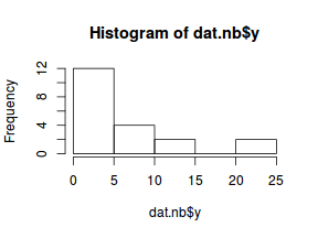
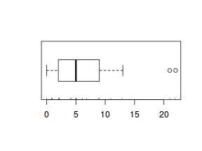
Check the distribution of the $y$ abundances
hist(dat.nb$y)
boxplot(dat.nb$y, horizontal=TRUE)
rug(jitter(dat.nb$y))
Confirm linearity
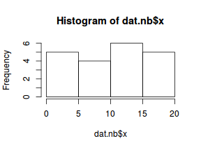
Lets now explore linearity by creating a histogram of the predictor variable ($x$) and a scatterplot of the relationship between the response ($y$) and the predictor ($x$)
hist(dat.nb$x)
#now for the scatterplot
plot(y~x, dat.nb, log="y")
with(dat.nb, lines(lowess(y~x)))
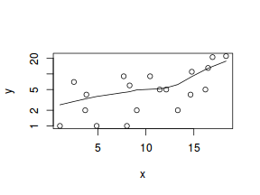
Conclusions: the predictor ($x$) does not display any skewness or other issues that might lead to non-linearity. The lowess smoother on the scatterplot does not display major deviations from a straight line and thus linearity is satisfied. Violations of linearity could be addressed by either:
- define a non-linear linear predictor (such as a polynomial, spline or other non-linear function)
- transform the scale of the predictor variables
Explore zero inflation
Although we have already established that there are few zeros in the data (and thus overdispersion is unlikely to be an issue), we can also explore this by comparing the number of zeros in the data to the number of zeros that would be expected from a Poisson distribution with a mean equal to the mean count of the data.
#proportion of 0's in the data
dat.nb.tab<-table(dat.nb$y==0)
dat.nb.tab/sum(dat.nb.tab)
FALSE  TRUE
 0.95  0.05
#proportion of 0's expected from a Poisson distribution
mu <- mean(dat.nb$y)
cnts <- rpois(1000, mu)
dat.nb.tabE <- table(cnts == 0)
dat.nb.tabE/sum(dat.nb.tabE)
FALSE
    1
Model fitting or statistical analysis
The boxplot of $y$ with the axis rug suggested that there might be some clumping (possibly due to some other unmeasured influence). It is therefore likely that the data are overdispersed.
dat.nb.list <- with(dat.nb,list(Y=y, X=x,N=nrow(dat.nb)))
modelString="
model {
  for (i in 1:N) {
     Y[i] ~ dpois(lambda[i])
     eta[i] <- beta0 + beta1*X[i]
     log(lambda[i]) <- eta[i]
  }
  beta0 ~ dnorm(0,1.0E-06)
  beta1 ~ dnorm(0,1.0E-06)
}
"
writeLines(modelString,con='../downloads/BUGSscripts/tut11.5bS3.4.bug')
library(R2jags)
system.time(
dat.nb.P.jags <- jags(model='../downloads/BUGSscripts/tut11.5bS3.4.bug', data=dat.nb.list, inits=NULL,
          param=c('beta0','beta1'),
          n.chain=3,
          n.iter=20000, n.thin=10, n.burnin=10000)
  )
Compiling model graph
   Resolving undeclared variables
   Allocating nodes
   Graph Size: 105

Initializing model
   user  system elapsed
  1.788   0.000   1.791
print(dat.nb.P.jags)
Inference for Bugs model at "../downloads/BUGSscripts/tut11.5bS3.4.bug", fit using jags,
 3 chains, each with 20000 iterations (first 10000 discarded), n.thin = 10
 n.sims = 3000 iterations saved
         mu.vect sd.vect    2.5%     25%     50%     75%  97.5%  Rhat n.eff
beta0      0.555   0.278   0.002   0.365   0.568   0.736   1.08 1.003  1000
beta1      0.111   0.020   0.072   0.098   0.111   0.125   0.15 1.002  1400
deviance 135.489   4.131 133.269 133.849 134.697 136.261 141.07 1.010  2700

For each parameter, n.eff is a crude measure of effective sample size,
and Rhat is the potential scale reduction factor (at convergence, Rhat=1).

DIC info (using the rule, pD = var(deviance)/2)
pD = 8.5 and DIC = 144.0
DIC is an estimate of expected predictive error (lower deviance is better).
#extract the samples for the two model parameters
coefs <- dat.nb.P.jags$BUGSoutput$sims.matrix[,1:2]
Xmat <- model.matrix(~x, data=dat)
#expected values on a log scale
eta<-coefs %*% t(Xmat)
#expected value on response scale
lambda <- exp(eta)

Resid <- -1*sweep(lambda,2,dat.nb$y, '-')/sqrt(lambda)
RSS <- apply(Resid^2, 1, sum)
Disp <- RSS/(nrow(dat.nb)-ncol(coefs))
data.frame(Median=median(Disp), Mean=mean(Disp), HPDinterval(as.mcmc(Disp)), HPDinterval(as.mcmc(Disp),p=0.5))
     Median  Mean lower upper lower.1 upper.1
var1  3.147 3.243  2.63 4.002   2.786   3.252
The dispersion parameter was 3.2425024, indicating over three times more variability than would be expected for a Poisson distribution.
The data are thus over-dispersed. Given that this is unlikely to be due to zero inflation and the rug plot did suggest some level of clumping,
negative binomial regression would seem reasonable.
Model fitting or statistical analysis
JAGS
$$ \begin{align} Y_i&\sim{}NB(p_i,size) & (\text{response distribution})\\ p_i&=size/(size+\lambda_i)\\ log(\lambda_i)&=\eta_i & (\text{link function})\\ \eta_i&=\beta_0+\beta_1 X_i & (\text{linear predictor})\\ \beta_0, \beta_1&\sim{}\mathcal{N}(0,10000) & (\text{diffuse Bayesian prior})\\ size &\sim{}\mathcal{U}(0.001,1000)\\ \end{align} $$dat.nb.list <- with(dat.nb,list(Y=y, X=x,N=nrow(dat.nb))) modelString=" model { for (i in 1:N) { Y[i] ~ dnegbin(p[i],size) p[i] <- size/(size+lambda[i]) log(lambda[i]) <- beta0 + beta1*X[i] } beta0 ~ dnorm(0,1.0E-06) beta1 ~ dnorm(0,1.0E-06) size ~ dunif(0.001,1000) theta <- pow(1/mean(p),2) scaleparam <- mean((1-p)/p) } " writeLines(modelString,con='../downloads/BUGSscripts/tut11.5bS4.1.bug') library(R2jags) system.time( dat.NB.jags <- jags(model='../downloads/BUGSscripts/tut11.5bS4.1.bug', data=dat.nb.list, inits=NULL, param=c('beta0','beta1', 'size','theta','scaleparam'), n.chain=3, n.iter=20000, n.thin=10, n.burnin=10000) )
Compiling model graph
   Resolving undeclared variables
   Allocating nodes
   Graph Size: 157

Initializing model
   user  system elapsed
 17.430   0.008  17.455
Xmat <- model.matrix(~x, dat.nb)
nX <- ncol(Xmat)
dat.nb.list1 <- with(dat.nb,list(Y=y, X=Xmat,N=nrow(dat.nb), nX=nX))
modelString="
model {
  for (i in 1:N) {
     Y[i] ~ dnegbin(p[i],size)
     p[i] <- size/(size+lambda[i])
     eta[i] <- inprod(beta[], X[i,])
     log(lambda[i]) <- max(-20,min(20,eta[i]))
  }
  for (i in 1:nX) {
    beta[i] ~ dnorm(0,1.0E-06)
  }
  size ~ dunif(0.001,10000)
}
"
writeLines(modelString,con='../downloads/BUGSscripts/tut11.5bS4.11.bug')
library(R2jags)
system.time(
dat.NB.jags1 <- jags(model='../downloads/BUGSscripts/tut11.5bS4.11.bug', data=dat.nb.list1, inits=NULL,
          param=c('beta'),
          n.chain=3,
          n.iter=20000, n.thin=10, n.burnin=10000)
  )
Compiling model graph
   Resolving undeclared variables
   Allocating nodes
   Graph Size: 212

Initializing model
   user  system elapsed
  17.01    0.00   17.02
print(dat.NB.jags1)
Inference for Bugs model at "../downloads/BUGSscripts/tut11.5bS4.11.bug", fit using jags,
 3 chains, each with 20000 iterations (first 10000 discarded), n.thin = 10
 n.sims = 3000 iterations saved
         mu.vect sd.vect    2.5%     25%     50%     75%   97.5%  Rhat n.eff
beta[1]    0.733   0.415  -0.069   0.465   0.725   1.005   1.564 1.001  3000
beta[2]    0.097   0.033   0.032   0.075   0.097   0.118   0.163 1.001  3000
deviance 113.046   2.682 110.080 111.088 112.321 114.261 120.171 1.002  2000

For each parameter, n.eff is a crude measure of effective sample size,
and Rhat is the potential scale reduction factor (at convergence, Rhat=1).

DIC info (using the rule, pD = var(deviance)/2)
pD = 3.6 and DIC = 116.6
DIC is an estimate of expected predictive error (lower deviance is better).
Or arguably better still, use a multivariate normal prior. If we have a $k$ regression parameters ($\beta_k$), then the multivariate normal priors are defined as: $$ \boldsymbol{\beta}\sim{}\mathcal{N_k}(\boldsymbol{\mu}, \mathbf{\Sigma}) $$ where $$\boldsymbol{\mu}=[E[\beta_1],E[\beta_2],...,E[\beta_k]] = \left(\begin{array}{c}0\\\vdots\\0\end{array}\right)$$ $$ \mathbf{\Sigma}=[Cov[\beta_i, \beta_j]] = \left(\begin{array}{ccc}1000^2&0&0\\0&\ddots&0\\0&0&1000^2\end{array} \right) $$ hence, along with the response and predictor matrix, we need to supply $\boldsymbol{\mu}$ (a vector of zeros) and $\boldsymbol{\Sigma}$ (a covariance matrix with $1000^2$ in the diagonals).
Xmat <- model.matrix(~x, dat.nb)
nX <- ncol(Xmat)
dat.nb.list2 <- with(dat.nb,list(Y=y, X=Xmat,N=nrow(dat.nb), mu=rep(0,nX),Sigma=diag(1.0E-06,nX)))
modelString="
model {
  for (i in 1:N) {
     Y[i] ~ dnegbin(p[i],size)
     p[i] <- size/(size+lambda[i])
     eta[i] <- inprod(beta[], X[i,])
     log(lambda[i]) <- eta[i]
  }
  beta ~ dmnorm(mu[],Sigma[,])
  size ~ dunif(0.001,10000)
}
"
writeLines(modelString,con='../downloads/BUGSscripts/tut11.5bS4.12.bug')
library(R2jags)
system.time(
dat.NB.jags2 <- jags(model='../downloads/BUGSscripts/tut11.5bS4.12.bug', data=dat.nb.list2, inits=NULL,
          param=c('beta', 'size'),
          n.chain=3,
          n.iter=20000, n.thin=10, n.burnin=10000)
  )
Compiling model graph
   Resolving undeclared variables
   Allocating nodes
   Graph Size: 173

Initializing model
   user  system elapsed
  6.353   0.000   6.361
print(dat.NB.jags2)
Inference for Bugs model at "../downloads/BUGSscripts/tut11.5bS4.12.bug", fit using jags,
 3 chains, each with 20000 iterations (first 10000 discarded), n.thin = 10
 n.sims = 3000 iterations saved
         mu.vect sd.vect    2.5%     25%     50%     75%   97.5%  Rhat n.eff
beta[1]    0.737   0.421  -0.097   0.460   0.736   1.013   1.555 1.002  3000
beta[2]    0.097   0.033   0.030   0.076   0.097   0.118   0.164 1.001  3000
size       3.102   1.931   1.048   1.885   2.615   3.749   7.885 1.001  3000
deviance 113.067   2.628 110.066 111.150 112.407 114.255 120.059 1.002  1600

For each parameter, n.eff is a crude measure of effective sample size,
and Rhat is the potential scale reduction factor (at convergence, Rhat=1).

DIC info (using the rule, pD = var(deviance)/2)
pD = 3.5 and DIC = 116.5
DIC is an estimate of expected predictive error (lower deviance is better).
dat.nb.brm <- brm(y~x, data=dat.nb, family='negbinomial',
   prior=c(set_prior("normal(0,100)", class="b"),
           set_prior("student_t(3,0,5)", class="shape")),
   chains=3, iter=2000, warmup=1000, thin=2)
SAMPLING FOR MODEL 'negbinomial(log) brms-model' NOW (CHAIN 1).

Chain 1, Iteration:    1 / 2000 [  0%]  (Warmup)
Chain 1, Iteration:  200 / 2000 [ 10%]  (Warmup)
Chain 1, Iteration:  400 / 2000 [ 20%]  (Warmup)
Chain 1, Iteration:  600 / 2000 [ 30%]  (Warmup)
Chain 1, Iteration:  800 / 2000 [ 40%]  (Warmup)
Chain 1, Iteration: 1000 / 2000 [ 50%]  (Warmup)
Chain 1, Iteration: 1001 / 2000 [ 50%]  (Sampling)
Chain 1, Iteration: 1200 / 2000 [ 60%]  (Sampling)
Chain 1, Iteration: 1400 / 2000 [ 70%]  (Sampling)
Chain 1, Iteration: 1600 / 2000 [ 80%]  (Sampling)
Chain 1, Iteration: 1800 / 2000 [ 90%]  (Sampling)
Chain 1, Iteration: 2000 / 2000 [100%]  (Sampling)#
#  Elapsed Time: 0.129428 seconds (Warm-up)
#                0.100482 seconds (Sampling)
#                0.22991 seconds (Total)
#

SAMPLING FOR MODEL 'negbinomial(log) brms-model' NOW (CHAIN 2).

Chain 2, Iteration:    1 / 2000 [  0%]  (Warmup)
Chain 2, Iteration:  200 / 2000 [ 10%]  (Warmup)
Chain 2, Iteration:  400 / 2000 [ 20%]  (Warmup)
Chain 2, Iteration:  600 / 2000 [ 30%]  (Warmup)
Chain 2, Iteration:  800 / 2000 [ 40%]  (Warmup)
Chain 2, Iteration: 1000 / 2000 [ 50%]  (Warmup)
Chain 2, Iteration: 1001 / 2000 [ 50%]  (Sampling)
Chain 2, Iteration: 1200 / 2000 [ 60%]  (Sampling)
Chain 2, Iteration: 1400 / 2000 [ 70%]  (Sampling)
Chain 2, Iteration: 1600 / 2000 [ 80%]  (Sampling)
Chain 2, Iteration: 1800 / 2000 [ 90%]  (Sampling)
Chain 2, Iteration: 2000 / 2000 [100%]  (Sampling)#
#  Elapsed Time: 0.11 seconds (Warm-up)
#                0.091671 seconds (Sampling)
#                0.201671 seconds (Total)
#

SAMPLING FOR MODEL 'negbinomial(log) brms-model' NOW (CHAIN 3).

Chain 3, Iteration:    1 / 2000 [  0%]  (Warmup)
Chain 3, Iteration:  200 / 2000 [ 10%]  (Warmup)
Chain 3, Iteration:  400 / 2000 [ 20%]  (Warmup)
Chain 3, Iteration:  600 / 2000 [ 30%]  (Warmup)
Chain 3, Iteration:  800 / 2000 [ 40%]  (Warmup)
Chain 3, Iteration: 1000 / 2000 [ 50%]  (Warmup)
Chain 3, Iteration: 1001 / 2000 [ 50%]  (Sampling)
Chain 3, Iteration: 1200 / 2000 [ 60%]  (Sampling)
Chain 3, Iteration: 1400 / 2000 [ 70%]  (Sampling)
Chain 3, Iteration: 1600 / 2000 [ 80%]  (Sampling)
Chain 3, Iteration: 1800 / 2000 [ 90%]  (Sampling)
Chain 3, Iteration: 2000 / 2000 [100%]  (Sampling)#
#  Elapsed Time: 0.108511 seconds (Warm-up)
#                0.074716 seconds (Sampling)
#                0.183227 seconds (Total)
#
Chain mixing and Model validation
Prior to exploring the model parameters, it is prudent to confirm that the model did indeed fit the assumptions and was an appropriate fit to the data as well as that the MCMC sampling chain was adequately mixed and the retained samples independent.
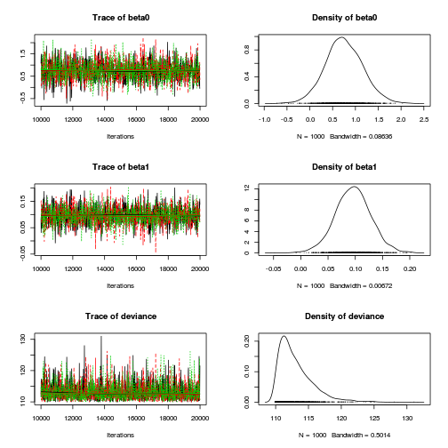
- We will start by exploring the mixing of the MCMC chains via traceplots.
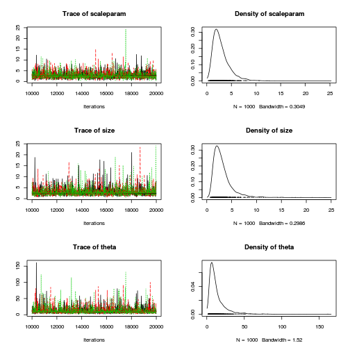
plot(as.mcmc(dat.NB.jags))
library(gridExtra)
grid.arrange(stan_trace(dat.nb.brm$fit, ncol=1),
             stan_dens(dat.nb.brm$fit, separate_chains=TRUE,ncol=1),
             ncol=2)
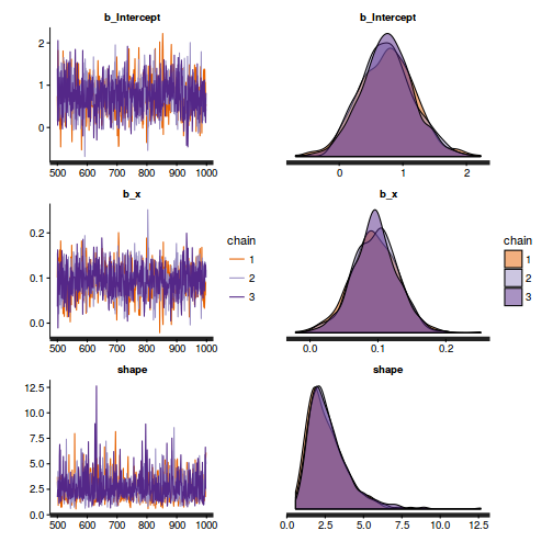
The chains appear well mixed and stable
- Next we will explore correlation amongst MCMC samples.
autocorr.diag(as.mcmc(dat.NB.jags))
           beta0    beta1   deviance scaleparam     size     theta
Lag 0    1.00000  1.00000  1.0000000  1.0000000  1.00000  1.000000
Lag 10   0.30859  0.30371  0.0455964  0.0180221  0.08759  0.028477
Lag 50  -0.05370 -0.05565  0.0011639 -0.0206865 -0.01812 -0.022056
Lag 100 -0.01028 -0.01914 -0.0003804 -0.0075196  0.01651 -0.004871
Lag 500  0.02130  0.01817 -0.0441559  0.0001324  0.01337  0.022265
The level of auto-correlation at the nominated lag of 10 is higher than we would generally like. It is worth increasing the thinning rate from 10 to 50. Obviously, to support this higher thinning rate, we would also increase the number of iterations. Typically for a negative binomial, it is worth having a large burnin (approximately half of the iterations).
library(R2jags)
dat.NB.jags <- jags(data=dat.nb.list,model.file='../downloads/BUGSscripts/tut11.5bS4.1.bug',
                   param=c('beta0','beta1','size'),
                   n.chains=3, n.iter=50000, n.burnin=25000, n.thin=50)
Compiling model graph
   Resolving undeclared variables
   Allocating nodes
   Graph Size: 157

Initializing model
print(dat.NB.jags)
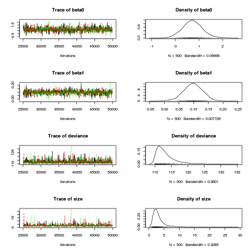
Inference for Bugs model at "../downloads/BUGSscripts/tut11.5bS4.1.bug", fit using jags, 3 chains, each with 50000 iterations (first 25000 discarded), n.thin = 50 n.sims = 1500 iterations saved mu.vect sd.vect 2.5% 25% 50% 75% 97.5% Rhat n.eff beta0 0.730 0.421 -0.074 0.452 0.725 0.996 1.602 1.000 1500 beta1 0.097 0.033 0.030 0.077 0.098 0.119 0.157 1.001 1500 size 3.167 2.185 1.086 1.911 2.641 3.704 8.551 1.002 1100 deviance 113.089 2.760 110.053 111.122 112.340 114.179 120.468 1.004 780 For each parameter, n.eff is a crude measure of effective sample size, and Rhat is the potential scale reduction factor (at convergence, Rhat=1). DIC info (using the rule, pD = var(deviance)/2) pD = 3.8 and DIC = 116.9 DIC is an estimate of expected predictive error (lower deviance is better).plot(as.mcmc(dat.NB.jags))
autocorr.diag(as.mcmc(dat.NB.jags))
             beta0     beta1  deviance     size
Lag 0     1.000000  1.000000  1.000000  1.00000
Lag 50    0.002132  0.007780  0.002472  0.00480
Lag 250  -0.014601 -0.013641 -0.012261 -0.06051
Lag 500   0.019129  0.015262 -0.023785  0.01291
Lag 2500  0.039030  0.008195 -0.013073 -0.01248
Conclusions: the samples are now less auto-correlated. Ideally, we should probably collect even more samples. Whilst the traceplots are reasonably noisy, there is more of a signal or pattern than there ideally should be.
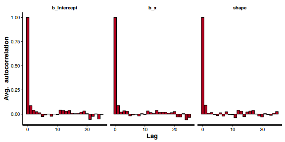
stan_ac(dat.nb.brm$fit)
- Explore the step size characteristics (STAN only)
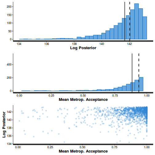
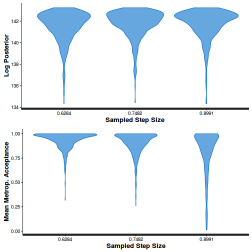
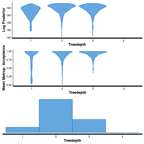
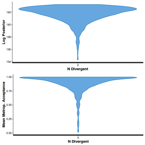
Conclusions: acceptance ratio is very good, the lot posterior is relatively robust to step size and tree depth, rhat values are all below 1.05, the effective sample size is always above 0.5 and the ratio of MCMC error to posterior sd is very small.
summary(do.call(rbind, args = get_sampler_params(dat.nb.brm$fit, inc_warmup = FALSE)), digits = 2)
 accept_stat__     stepsize__    treedepth__   n_leapfrog__  n_divergent__
 Min.   :0.012   Min.   :0.63   Min.   :1.0   Min.   : 1.0   Min.   :0
 1st Qu.:0.850   1st Qu.:0.63   1st Qu.:2.0   1st Qu.: 3.0   1st Qu.:0
 Median :0.937   Median :0.75   Median :2.0   Median : 3.0   Median :0
 Mean   :0.884   Mean   :0.76   Mean   :2.2   Mean   : 3.8   Mean   :0
 3rd Qu.:0.990   3rd Qu.:0.90   3rd Qu.:3.0   3rd Qu.: 5.0   3rd Qu.:0
 Max.   :1.000   Max.   :0.90   Max.   :4.0   Max.   :15.0   Max.   :0
stan_diag(dat.nb.brm$fit)
stan_diag(dat.nb.brm$fit, information = "stepsize")
stan_diag(dat.nb.brm$fit, information = "treedepth")
stan_diag(dat.nb.brm$fit, information = "divergence")
library(gridExtra)
grid.arrange(stan_rhat(dat.nb.brm$fit) + theme_classic(8),
             stan_ess(dat.nb.brm$fit) + theme_classic(8),
             stan_mcse(dat.nb.brm$fit) + theme_classic(8),
             ncol = 2)
- We now explore the goodness of fit of the models via the residuals and deviance.
We could calculate the Pearsons's residuals within the JAGS model.
Alternatively, we could use the parameters to generate the residuals outside of JAGS.
#extract the samples for the two model parameters
coefs <- dat.NB.jags$BUGSoutput$sims.matrix[,1:2]
size <- dat.NB.jags$BUGSoutput$sims.matrix[,'size']
Xmat <- model.matrix(~x, data=dat.nb)
#expected values on a log scale
eta<-coefs %*% t(Xmat)
#expected value on response scale
lambda <- exp(eta)
varY <- lambda + (lambda^2)/size
#sweep across rows and then divide by lambda
Resid <- -1*sweep(lambda,2,dat.nb$y,'-')/sqrt(varY)
#plot residuals vs expected values
plot(apply(Resid,2,mean)~apply(eta,2,mean))

#Calculate residuals
Resid.nb.brm <- residuals(dat.nb.brm, type='pearson')
Fitted.nb.brm <- fitted(dat.nb.brm, scale='linear')
ggplot(data=NULL, aes(y=Resid.nb.brm[,'Estimate'], x=Fitted.nb.brm[,'Estimate'])) + geom_point()
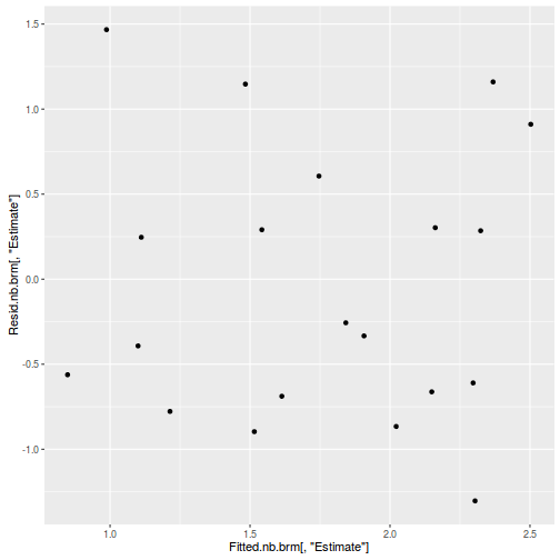
There are no real patterns in the residuals.
- Now we will compare the sum of squared residuals to the sum of squares residuals that would be expected from a Poisson distribution
matching that estimated by the model. Essentially this is estimating how well the Poisson distribution, the log-link function and the linear model
approximates the observed data.
SSres<-apply(Resid^2,1,sum)

set.seed(2)
#generate a matrix of draws from a negative binomial distribution
# the matrix is the same dimensions as pi and uses the probabilities of pi
YNew <- matrix(rnbinom(length(lambda),mu=lambda, size=size),nrow=nrow(lambda))
Resid1<-(lambda - YNew)/sqrt(varY)
SSres.sim<-apply(Resid1^2,1,sum)
mean(SSres.sim>SSres)
[1] 0.4127
Xmat <- model.matrix(~x, dat.nb)
nX <- ncol(Xmat)
dat.nb.list2 <- with(dat.nb,list(Y=y, X=Xmat,N=nrow(dat.nb), mu=rep(0,nX),Sigma=diag(1.0E-06,nX)))
modelString="
model {
  for (i in 1:N) {
     Y[i] ~ dnegbin(p[i],size)
     p[i] <- size/(size+lambda[i])
     eta[i] <- inprod(beta[], X[i,])
     log(lambda[i]) <- eta[i]

     Y1[i] ~ dnegbin(p[i],size)
	 varY[i] <- lambda[i] + pow(lambda[i],2)/size
	 Resid[i] <- (Y[i] - lambda[i])/sqrt(varY[i])
     Resid1[i] <- (Y1[i] - lambda[i])/sqrt(varY[i])
     RSS[i] <- pow(Resid[i],2)
     RSS1[i] <-pow(Resid1[i],2)
  }
  beta ~ dmnorm(mu[],Sigma[,])
  size ~ dunif(0.001,10000)
  Pvalue <- mean(sum(RSS1)>sum(RSS))
}
"
writeLines(modelString,con='../downloads/BUGSscripts/tut11.5bS4.61.bug')
library(R2jags)
system.time(
dat.NB.jags3 <- jags(model='../downloads/BUGSscripts/tut11.5bS4.61.bug', data=dat.nb.list2, inits=NULL,
          param=c('beta','Pvalue'),
          n.chain=3,
          n.iter=20000, n.thin=10, n.burnin=10000)
  )
Compiling model graph
   Resolving undeclared variables
   Allocating nodes
   Graph Size: 400

Initializing model
   user  system elapsed
  6.717   0.000   6.726
print(dat.NB.jags3)
Inference for Bugs model at "../downloads/BUGSscripts/tut11.5bS4.61.bug", fit using jags, 3 chains, each with 20000 iterations (first 10000 discarded), n.thin = 10 n.sims = 3000 iterations saved mu.vect sd.vect 2.5% 25% 50% 75% 97.5% Rhat n.eff Pvalue 0.421 0.494 0.000 0.000 0.000 1.000 1.000 1.002 1000 beta[1] 0.763 0.422 -0.035 0.482 0.746 1.044 1.619 1.002 1400 beta[2] 0.095 0.033 0.030 0.072 0.095 0.117 0.160 1.002 1500 deviance 113.064 2.596 110.071 111.143 112.361 114.276 119.730 1.001 3000 For each parameter, n.eff is a crude measure of effective sample size, and Rhat is the potential scale reduction factor (at convergence, Rhat=1). DIC info (using the rule, pD = var(deviance)/2) pD = 3.4 and DIC = 116.4 DIC is an estimate of expected predictive error (lower deviance is better).Resid.nb.brm <- residuals(dat.nb.brm, type='pearson', summary=FALSE) SSres.nb.brm <- apply(Resid.nb.brm^2,1,sum) lambda.nb.brm = fitted(dat.nb.brm, scale='response', summary=FALSE) YNew.nb.brm <- matrix(rpois(length(lambda.nb.brm), lambda=lambda.nb.brm),nrow=nrow(lambda.nb.brm)) Resid1.nb.brm<-(lambda.nb.brm - YNew.nb.brm)/sqrt(lambda.nb.brm) SSres.sim.nb.brm<-apply(Resid1.nb.brm^2,1,sum) mean(SSres.sim.nb.brm>SSres.nb.brm)
[1] 0.8286667
Conclusions: the Bayesian p-value is not far from 0.5, suggesting that there is a good fit of the model to the data.
- Unfortunately, unlike with linear models (Gaussian family), the expected distribution of data (residuals) varies
over the range of fitted values for numerous (often competing) ways that make diagnosing (and attributing causes
thereof) miss-specified generalized linear models from standard residual plots very difficult. The use of standardized
(Pearson) residuals or deviance residuals can partly address this issue, yet they still do not offer completely
consistent diagnoses across all issues (miss-specified model, over-dispersion, zero-inflation).
An alternative approach is to use simulated data from the model posteriors to calculate an empirical cumulative density function from which residuals are are generated as values corresponding to the observed data along the density function.
The trend (black symbols) in the qq-plot does not appear to be overly non-linear (matching the ideal red line well), suggesting that the model is not overdispersed. The spread of standardized (simulated) residuals in the residual plot do not appear overly non-uniform. That is there is not trend in the residuals. Furthermore, there is not a concentration of points close to 1 or 0 (which would imply overdispersion).#extract the samples for the two model parameters coefs <- dat.NB.jags$BUGSoutput$sims.matrix[,1:2] size <- dat.NB.jags$BUGSoutput$sims.matrix[,'size'] Xmat <- model.matrix(~x, data=dat.nb) #expected values on a log scale eta<-coefs %*% t(Xmat) #expected value on response scale lambda <- exp(eta) simRes <- function(lambda, data,n=250, plot=T, family='negbin', size=NULL) { require(gap) N = nrow(data) sim = switch(family, 'poisson' = matrix(rpois(n*N,apply(lambda,2,mean)),ncol=N, byrow=TRUE), 'negbin' = matrix(MASS:::rnegbin(n*N,apply(lambda,2,mean),size),ncol=N, byrow=TRUE) ) a = apply(sim + runif(n,-0.5,0.5),2,ecdf) resid<-NULL for (i in 1:nrow(data)) resid<-c(resid,a[[i]](data$y[i] + runif(1 ,-0.5,0.5))) if (plot==T) { par(mfrow=c(1,2)) gap::qqunif(resid,pch = 2, bty = "n", logscale = F, col = "black", cex = 0.6, main = "QQ plot residuals", cex.main = 1, las=1) plot(resid~apply(lambda,2,mean), xlab='Predicted value', ylab='Standardized residual', las=1) } resid } simRes(lambda,dat.nb, family='negbin', size=mean(size))
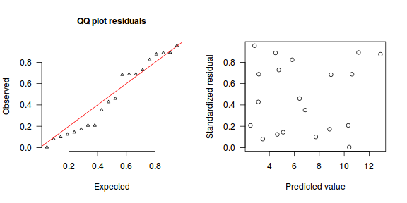
[1] 0.208 0.956 0.428 0.688 0.080 0.888 0.124 0.728 0.144 0.824 0.460 0.352 0.100 0.172 0.684 0.208 0.004 0.688 0.892 0.876
lambda.nb.brm = fitted(dat.nb.brm, scale='response', summary=FALSE)
size <- as.matrix(as.data.frame(rstan:::extract(dat.nb.brm$fit, par='shape')))

simRes <- function(lambda, data,n=250, plot=T, family='poisson', size=NULL) {
 require(gap)
 N = nrow(data)
 sim = switch(family,
    'poisson' = matrix(rpois(n*N,apply(lambda,2,mean)),ncol=N, byrow=TRUE),
    'negbin' = matrix(MASS:::rnegbin(n*N,apply(lambda,2,mean),size),ncol=N, byrow=TRUE)
 )
 a = apply(sim + runif(n,-0.5,0.5),2,ecdf)
 resid<-NULL
 for (i in 1:nrow(data)) resid<-c(resid,a[[i]](data$y[i] + runif(1 ,-0.5,0.5)))
 if (plot==T) {
   par(mfrow=c(1,2))
   gap::qqunif(resid,pch = 2, bty = "n",
   logscale = F, col = "black", cex = 0.6, main = "QQ plot residuals",
   cex.main = 1, las=1)
   plot(resid~apply(lambda,2,mean), xlab='Predicted value', ylab='Standardized residual', las=1)
 }
 resid
}

simRes(lambda.nb.brm, dat.nb, family='negbin', size=mean(size))
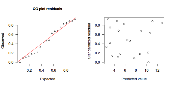
[1] 0.332 0.924 0.420 0.748 0.128 0.888 0.108 0.680 0.184 0.824 0.480 0.464 0.092 0.180 0.672 0.212 0.000 0.628 0.884 0.844
Exploring the model parameters, test hypotheses
If there was any evidence that the assumptions had been violated or the model was not an appropriate fit, then we would need to reconsider the model and start the process again. In this case, there is no evidence that the test will be unreliable so we can proceed to explore the test statistics.
As with most Bayesian models, it is best to base conclusions on medians rather than means.
print(dat.NB.jags)
Inference for Bugs model at "../downloads/BUGSscripts/tut11.5bS4.1.bug", fit using jags,
 3 chains, each with 50000 iterations (first 25000 discarded), n.thin = 50
 n.sims = 1500 iterations saved
         mu.vect sd.vect    2.5%     25%     50%     75%   97.5%  Rhat n.eff
beta0      0.730   0.421  -0.074   0.452   0.725   0.996   1.602 1.000  1500
beta1      0.097   0.033   0.030   0.077   0.098   0.119   0.157 1.001  1500
size       3.167   2.185   1.086   1.911   2.641   3.704   8.551 1.002  1100
deviance 113.089   2.760 110.053 111.122 112.340 114.179 120.468 1.004   780

For each parameter, n.eff is a crude measure of effective sample size,
and Rhat is the potential scale reduction factor (at convergence, Rhat=1).

DIC info (using the rule, pD = var(deviance)/2)
pD = 3.8 and DIC = 116.9
DIC is an estimate of expected predictive error (lower deviance is better).
library(plyr)
adply(dat.NB.jags$BUGSoutput$sims.matrix, 2, function(x) {
  data.frame(Median=median(x), Mean=mean(x), HPDinterval(as.mcmc(x)), HPDinterval(as.mcmc(x),p=0.5))
})
        X1    Median      Mean     lower    upper   lower.1  upper.1
1    beta0   0.72460   0.72989  -0.08683   1.5612   0.40701   0.9444
2    beta1   0.09763   0.09734   0.03644   0.1629   0.07544   0.1171
3 deviance 112.34047 113.08851 109.87327 118.6993 110.36278 112.7765
4     size   2.64119   3.16733   0.64845   7.0820   1.21209   2.7610
Actually, many find it more palatable to express the estimates in the original scale of the observations rather than on a log scale.
library(plyr)
adply(exp(dat.NB.jags$BUGSoutput$sims.matrix[,1:2]), 2, function(x) {
  data.frame(Median=median(x), Mean=mean(x), HPDinterval(as.mcmc(x)), HPDinterval(as.mcmc(x),p=0.5))
})
     X1 Median  Mean  lower upper lower.1 upper.1
1 beta0  2.064 2.274 0.7971 4.352   1.353   2.368
2 beta1  1.103 1.103 1.0307 1.170   1.078   1.124
Conclusions:
We would reject the null hypothesis of no effect of $x$ on $y$.
An increase in x is associated with a significant linear increase (positive slope) in the abundance of $y$.
Every 1 unit increase in $x$ results in a log 0.0976275 unit increase in $y$.
We usually express this in terms of abundance rather than log abundance, so
every 1 unit increase in $x$ results in a ($e^{0.0976275}=1.1025521$)
1.1025521 unit increase in the abundance of $y$.
summary(dat.nb.brm)
 Family: negbinomial (log)
Formula: y ~ x
   Data: dat.nb (Number of observations: 20)
Samples: 3 chains, each with iter = 2000; warmup = 1000; thin = 2;
         total post-warmup samples = 1500
   WAIC: Not computed

Fixed Effects:
          Estimate Est.Error l-95% CI u-95% CI Eff.Sample Rhat
Intercept     0.75      0.42    -0.04     1.59       1124    1
x             0.10      0.03     0.03     0.16       1110    1

Family Specific Parameters:
      Estimate Est.Error l-95% CI u-95% CI Eff.Sample Rhat
shape     2.64      1.27     0.93     5.76       1214    1

Samples were drawn using sampling(NUTS). For each parameter, Eff.Sample
is a crude measure of effective sample size, and Rhat is the potential
scale reduction factor on split chains (at convergence, Rhat = 1).
exp(coef(dat.nb.brm))
              mean
Intercept 2.114221
x         1.100268
coefs.nb.brm <- as.matrix(as.data.frame(rstan:::extract(dat.nb.brm$fit)))
coefs.nb.brm <- coefs.nb.brm[,grep('b', colnames(coefs.nb.brm))]
plyr:::adply(exp(coefs.nb.brm), 2, function(x) {
  data.frame(Mean=mean(x), median=median(x), HPDinterval(as.mcmc(x)))
  })
           X1     Mean   median     lower    upper
1 b_Intercept 2.312289 2.123695 0.8215863 4.460667
2         b_x 1.100884 1.100589 1.0281742 1.173267
marginal_effects(dat.nb.brm)
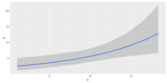
Further explorations of the trends
A measure of the strength of the relationship can be obtained according to: $$R^2 = 1 - \frac{RSS_{model}}{RSS_{null}}$$
Xmat <- model.matrix(~x, data=dat.nb)
#expected values on a log scale
eta<-coefs %*% t(Xmat)
#expected value on response scale
lambda <- exp(eta)
#calculate the raw SS residuals
SSres <- apply((-1*(sweep(lambda,2,dat.nb$y,'-')))^2,1,sum)
SSres.null <- sum((dat.nb$y - mean(dat.nb$y))^2)
#OR
SSres.null <- crossprod(dat.nb$y - mean(dat.nb$y))
#calculate the model r2
1-mean(SSres)/SSres.null
       [,1]
[1,] 0.2719
Conclusions: 27.19% of the variation in $y$ abundance can be explained by its relationship with $x$.
Xmat <- model.matrix(~x, dat.nb)
nX <- ncol(Xmat)
dat.nb.list2 <- with(dat.nb,list(Y=y, X=Xmat,N=nrow(dat.nb), mu=rep(0,nX),Sigma=diag(1.0E-06,nX)))
modelString="
model {
  for (i in 1:N) {
     Y[i] ~ dnegbin(p[i],size)
     p[i] <- size/(size+lambda[i])
     eta[i] <- inprod(beta[], X[i,])
     log(lambda[i]) <- eta[i]

     res[i] <- Y[i] - lambda[i]
     resnull[i] <- Y[i] - meanY
  }
  meanY <- mean(Y)
  beta ~ dmnorm(mu[],Sigma[,])
  size ~ dunif(0.001,10000)
  RSS <- sum(res^2)
  RSSnull <- sum(resnull^2)
  r2 <- 1-RSS/RSSnull
}
"
writeLines(modelString,con='../downloads/BUGSscripts/tut11.5bS4.9.bug')
library(R2jags)
system.time(
dat.NB.jags4 <- jags(model='../downloads/BUGSscripts/tut11.5bS4.9.bug', data=dat.nb.list2, inits=NULL,
          param=c('beta','r2'),
          n.chain=3,
          n.iter=20000, n.thin=10, n.burnin=10000)
  )
Compiling model graph
   Resolving undeclared variables
   Allocating nodes
   Graph Size: 217

Initializing model
   user  system elapsed
  6.181   0.000   6.191
print(dat.NB.jags4)
Inference for Bugs model at "../downloads/BUGSscripts/tut11.5bS4.9.bug", fit using jags,
 3 chains, each with 20000 iterations (first 10000 discarded), n.thin = 10
 n.sims = 3000 iterations saved
         mu.vect sd.vect    2.5%     25%     50%     75%   97.5%  Rhat n.eff
beta[1]    0.727   0.405  -0.073   0.463   0.730   0.989   1.529 1.001  3000
beta[2]    0.097   0.032   0.034   0.076   0.097   0.117   0.163 1.002  1500
r2         0.276   0.148  -0.029   0.245   0.310   0.352   0.390 1.001  3000
deviance 113.051   2.625 110.048 111.134 112.366 114.231 120.033 1.001  3000

For each parameter, n.eff is a crude measure of effective sample size,
and Rhat is the potential scale reduction factor (at convergence, Rhat=1).

DIC info (using the rule, pD = var(deviance)/2)
pD = 3.4 and DIC = 116.5
DIC is an estimate of expected predictive error (lower deviance is better).
## calculate the expected values on the response scale
lambda.nb.brm = fitted(dat.nb.brm, scale='response', summary=FALSE)
## calculate the raw SSresid
SSres.nb.brm <- apply((-1*(sweep(lambda.nb.brm,2,dat.nb$y,'-')))^2,1,sum)
SSres.null <- sum((dat.nb$y - mean(dat.nb$y))^2)
#OR
SSres.null <- crossprod(dat.nb$y - mean(dat.nb$y))
#calculate the model r2
1-mean(SSres.nb.brm)/SSres.null
          [,1]
[1,] 0.2601319
Finally, we will create a summary plot.
par(mar = c(4, 5, 0, 0))
plot(y ~ x, data = dat.nb, type = "n", ann = F, axes = F)
points(y ~ x, data = dat.nb, pch = 16)
xs <- seq(min(dat.nb$x,na.rm=TRUE),max(dat.nb$x,na.rm=TRUE), l = 1000)
Xmat <- model.matrix(~xs)
eta<-coefs %*% t(Xmat)
ys <- exp(eta)
library(plyr)
library(coda)
data.tab <- adply(ys,2,function(x) {
  data.frame(Median=median(x), HPDinterval(as.mcmc(x)))
})
data.tab <- cbind(x=xs,data.tab)
points(Median ~ x, data=data.tab,col = "black", type = "l")
lines(lower ~ x, data=data.tab,col = "black", type = "l", lty = 2)
lines(upper ~ x, data=data.tab,col = "black", type = "l", lty = 2)

axis(1)
mtext("X", 1, cex = 1.5, line = 3)
axis(2, las = 2)
mtext("Abundance of Y", 2, cex = 1.5, line = 3)
box(bty = "l")
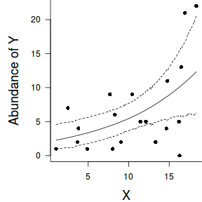
newdata = data.frame(x=seq(min(dat.nb$x), max(dat.nb$x), len=100))
Xmat = model.matrix(~x, data=newdata)
coefs <- as.matrix(as.data.frame(rstan:::extract(dat.nb.brm$fit)))
coefs <- coefs[,grep('b', colnames(coefs))]
fit = exp(coefs %*% t(Xmat))
newdata = cbind(newdata,
                plyr:::adply(fit, 2, function(x) {
                                  data.frame(Mean=mean(x), Median=median(x),
                                             HPDinterval(as.mcmc(x)))
                                })
)

ggplot(newdata, aes(y=Mean, x=x)) +
  geom_point(data=dat.nb, aes(y=y)) +
  geom_ribbon(aes(ymin=lower, ymax=upper), fill='blue',alpha=0.2) +
  geom_line() +
  scale_x_continuous('X') +
  scale_y_continuous('Abundance of Y') +
  theme_classic() +
  theme(axis.line.x=element_line(),axis.line.y=element_line())
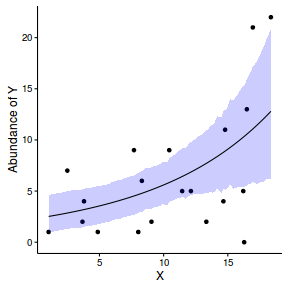
Defining full log-likelihood function
Now lets try it by specifying log-likelihood and the zero trick. When applying this trick, we need to manually calculate the deviance as the inbuilt deviance will be based on the log-likelihood of estimating the zeros (as part of the zero trick) rather than the deviance of the intended model..
The one advantage of the zero trick is that the Deviance and thus DIC, AIC provided by R2jags will be incorrect. Hence, they too need to be manually defined within jags. I suspect that the AIC calculation I have used is incorrect...
Xmat <- model.matrix(~x, dat.nb)
nX <- ncol(Xmat)
dat.nb.list2 <- with(dat.nb,list(Y=y, X=Xmat,N=nrow(dat.nb), mu=rep(0,nX),
                  Sigma=diag(1.0E-06,nX), zeros=rep(0,nrow(dat.nb)), C=10000))
modelString="
model {
  for (i in 1:N) {
     zeros[i] ~ dpois(zeros.lambda[i])
     zeros.lambda[i] <- -ll[i] + C
     ll[i] <- loggam(Y[i]+size) - loggam(Y[i]+1) - loggam(size) + size*(log(p[i]) - log(p[i]+1)) -
              Y[i]*log(p[i]+1)
     p[i] <- size/lambda[i]
     eta[i] <- inprod(beta[], X[i,])
     log(lambda[i]) <- eta[i]
  }
  beta ~ dmnorm(mu[],Sigma[,])
  size ~ dunif(0.001,1000)
  dev <- sum(-2*ll)
}
"
writeLines(modelString,con='../downloads/BUGSscripts/tut11.5bS4.14.bug')
library(R2jags)
system.time(
dat.NB.jags3 <- jags(model='../downloads/BUGSscripts/tut11.5bS4.14.bug', data=dat.nb.list2, inits=NULL,
          param=c('beta','dev'),
          n.chain=3,
          n.iter=50000, n.thin=50, n.burnin=10000)
  )
Compiling model graph
   Resolving undeclared variables
   Allocating nodes
   Graph Size: 453

Initializing model
   user  system elapsed
 16.996   0.000  17.014
print(dat.NB.jags3)
Inference for Bugs model at "../downloads/BUGSscripts/tut11.5bS4.14.bug", fit using jags,
 3 chains, each with 50000 iterations (first 10000 discarded), n.thin = 50
 n.sims = 2400 iterations saved
            mu.vect sd.vect       2.5%        25%        50%        75%      97.5%  Rhat n.eff
beta[1]       0.741   0.417     -0.074      0.461      0.738      1.020      1.559 1.002   990
beta[2]       0.096   0.033      0.033      0.074      0.097      0.118      0.160 1.003   640
dev         113.085   2.662    110.073    111.179    112.398    114.194    120.071 1.000  2400
deviance 400113.085   2.662 400110.073 400111.179 400112.398 400114.194 400120.071 1.000     1

For each parameter, n.eff is a crude measure of effective sample size,
and Rhat is the potential scale reduction factor (at convergence, Rhat=1).

DIC info (using the rule, pD = var(deviance)/2)
pD = 3.5 and DIC = 400116.6
DIC is an estimate of expected predictive error (lower deviance is better).
Zero-inflated Poisson (ZIP) regression
Zero-Inflation Poisson (ZIP) mixture model is defined as: $$ p(y_i|\theta,\lambda) = \left\{ \begin{array}{l l} \theta + (1-\theta)\times \text{Pois}(0|\lambda) & \quad \text{if $y_i=0$ and}\\ (1-\theta)\times \text{Pois}(y_i|\lambda) & \quad \text{if $y_i>0$} \end{array} \right. $$ where $\theta$ is the probability of false values (zeros).
Hence there is essentially two models coupled together (a mixture model) to yield an overall probability:
- when an observed response is zero ($y_i=0$), it is the probability of getting a false value (zero) plus the probability of a true value multiplied probability of drawing a value of zero from a Poisson distribution of $lambda$
- when an observed response is greater than 0, it is the probability of a true value multiplied probability of drawing that value from a Poisson distribution of $lambda$
The above formulation indicates the same $\lambda$ for both the zeros and non-zeros components. In the model of zero values, we are essentially investigating whether the likelihood of false zeros is related to the linear predictor and then the greater than zero model investigates whether the counts are related to the linear predictor.
However, we are typically less interested in modelling determinants of false zeros. Indeed, it is better that the likelihood of false zeros be unrelated to the linear predictor. For example, if excess (false zeros) are due to issues of detectability (individuals are present, just not detected), it is better that the detectability is not related to experimental treatments. Ideally, any detectability issues should be equal across all treatment levels.
The expected value of $Y$ and the variance in $Y$ for a ZIP model are: $$ E(y_i) = \lambda\times(1-\theta)\\ Var(y_i) = \lambda\times(1-\theta)\times(1+\theta\times\lambda^2) $$
Scenario and Data
Lets say we wanted to model the abundance of an item ($y$) against a continuous predictor ($x$). As this section is mainly about the generation of artificial data (and not specifically about what to do with the data), understanding the actual details are optional and can be safely skipped. Consequently, I have folded (toggled) this section away.
- the sample size = 20
- the continuous $x$ variable is a random uniform spread of measurements between 1 and 20
- the rate of change in log $y$ per unit of $x$ (slope) = 0.1.
- the value of $x$ when log$y$ equals 0 (when $y$=1)
- to generate the values of $y$ expected at each $x$ value, we evaluate the linear predictor (created by calculating the outer product of the model matrix and the regression parameters). These expected values are then transformed into a scale mapped by (0,$\infty$) by using the log function $e^{linear~predictor}$
- finally, we generate $y$ values by using the expected $y$ values ($\lambda$) as probabilities when drawing random numbers from a Poisson distribution. This step adds random noise to the expected $y$ values and returns only 0's and positive integers.
set.seed(37) #34.5  #4 #10 #16 #17 #26
#The number of samples
n.x <- 20
#Create x values that at uniformly distributed throughout the rate of 1 to 20
x <- sort(runif(n = n.x, min = 1, max =20))
mm <- model.matrix(~x)
intercept <- 0.6
slope=0.1
#The linear predictor
linpred <- mm %*% c(intercept,slope)
#Predicted y values
lambda <- exp(linpred)
#Add some noise and make binomial
library(gamlss.dist)
#fixed latent binomial
y<- rZIP(n.x,lambda, 0.4)
#latent binomial influenced by the linear predictor
#y<- rZIP(n.x,lambda, 1-exp(linpred)/(1+exp(linpred)))
dat.zip <- data.frame(y,x)

summary(glm(y~x, dat.zip, family="poisson"))
Call:
glm(formula = y ~ x, family = "poisson", data = dat.zip)

Deviance Residuals:
    Min       1Q   Median       3Q      Max
-2.5415  -2.3769  -0.9753   1.1736   3.6380

Coefficients:
            Estimate Std. Error z value Pr(>|z|)
(Intercept)  0.67048    0.33018   2.031   0.0423 *
x            0.02961    0.02663   1.112   0.2662
---
Signif. codes:  0 '***' 0.001 '**' 0.01 '*' 0.05 '.' 0.1 ' ' 1

(Dispersion parameter for poisson family taken to be 1)

    Null deviance: 85.469  on 19  degrees of freedom
Residual deviance: 84.209  on 18  degrees of freedom
AIC: 124.01

Number of Fisher Scoring iterations: 6
plot(glm(y~x, dat.zip, family="poisson"))
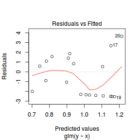
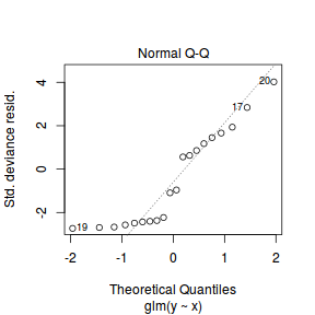
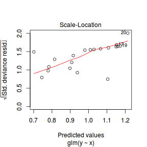
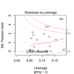
library(pscl)
summary(zeroinfl(y ~ x | 1, dist = "poisson", data = dat.zip))
Call:
zeroinfl(formula = y ~ x | 1, data = dat.zip, dist = "poisson")

Pearson residuals:
    Min      1Q  Median      3Q     Max
-1.0015 -0.9556 -0.3932  0.9663  1.6195

Count model coefficients (poisson with log link):
            Estimate Std. Error z value Pr(>|z|)
(Intercept)  0.70474    0.31960   2.205 0.027449 *
x            0.08734    0.02532   3.449 0.000563 ***

Zero-inflation model coefficients (binomial with logit link):
            Estimate Std. Error z value Pr(>|z|)
(Intercept)  -0.2292     0.4563  -0.502    0.615
---
Signif. codes:  0 '***' 0.001 '**' 0.01 '*' 0.05 '.' 0.1 ' ' 1

Number of iterations in BFGS optimization: 13
Log-likelihood: -36.17 on 3 Df
plot(resid(zeroinfl(y ~ x | 1, dist = "poisson", data = dat.zip))~fitted(zeroinfl(y ~ x | 1, dist = "poisson", data = dat.zip)))
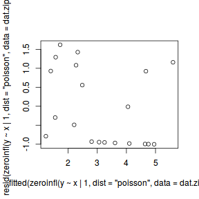
library(gamlss)
summary(gamlss(y~x,data=dat.zip, family=ZIP))
GAMLSS-RS iteration 1: Global Deviance = 72.4363
GAMLSS-RS iteration 2: Global Deviance = 72.3428
GAMLSS-RS iteration 3: Global Deviance = 72.3428
*******************************************************************
Family:  c("ZIP", "Poisson Zero Inflated")

Call:  gamlss(formula = y ~ x, family = ZIP, data = dat.zip)

Fitting method: RS()

-------------------------------------------------------------------
Mu link function:  log
Mu Coefficients:
            Estimate Std. Error t value Pr(>|t|)
(Intercept)  0.70582    0.31958   2.209  0.04123 *
x            0.08719    0.02533   3.442  0.00311 **
---
Signif. codes:  0 '***' 0.001 '**' 0.01 '*' 0.05 '.' 0.1 ' ' 1

-------------------------------------------------------------------
Sigma link function:  logit
Sigma Coefficients:
            Estimate Std. Error t value Pr(>|t|)
(Intercept)  -0.2292     0.4563  -0.502    0.622

-------------------------------------------------------------------
No. of observations in the fit:  20
Degrees of Freedom for the fit:  3
      Residual Deg. of Freedom:  17
                      at cycle:  3

Global Deviance:     72.34282
            AIC:     78.34282
            SBC:     81.33002
*******************************************************************
predict(gamlss(y~x,data=dat.zip, family=ZIP), se.fit=TRUE, what="mu")
GAMLSS-RS iteration 1: Global Deviance = 72.4363
GAMLSS-RS iteration 2: Global Deviance = 72.3428
GAMLSS-RS iteration 3: Global Deviance = 72.3428
$fit
        1         2         3         4         5         6         7         8         9        10        11        12        13        14        15        16        17        18        19        20
0.7966905 0.9236189 1.0263933 1.0369823 1.1305358 1.3763304 1.4054417 1.4299603 1.4951229 1.6161339 1.7035853 1.7629994 1.8678543 1.9838052 1.9951833 2.1187071 2.1249555 2.1431616 2.1837285 2.3064727

$se.fit
        1         2         3         4         5         6         7         8         9        10        11        12        13        14        15        16        17        18        19        20
0.3517894 0.3089432 0.2758980 0.2726011 0.2445792 0.1856062 0.1807322 0.1770893 0.1696661 0.1656458 0.1710016 0.1783138 0.1973009 0.2251987 0.2282363 0.2637860 0.2656903 0.2712879 0.2840032 0.3241532
Exploratory data analysis and initial assumption checking
- All of the observations are independent - this must be addressed at the design and collection stages
- The response variable (and thus the residuals) should be matched by an appropriate distribution (in the case of positive integers response - a Poisson is appropriate).
- All observations are equally influential in determining the trends - or at least no observations are overly influential. This is most effectively diagnosed via residuals and other influence indices and is very difficult to diagnose prior to analysis
- the relationship between the linear predictor (right hand side of the regression formula) and the link function should be linear. A scatterplot with smoother can be useful for identifying possible non-linearity.
- Dispersion is either 1 or overdispersion is otherwise accounted for in the model
- The number of zeros is either not excessive or else they are specifically addressed by the model
Confirm non-normality and explore clumping
Check the distribution of the $y$ abundances
hist(dat.zip$y)
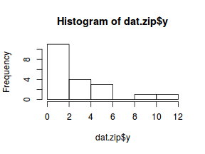
boxplot(dat.zip$y, horizontal=TRUE)
rug(jitter(dat.zip$y))
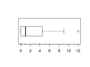
Confirm linearity
Lets now explore linearity by creating a histogram of the predictor variable ($x$). Note, it is difficult to directly assess issues of linearity. Indeed, a scatterplot with lowess smoother will be largely influenced by the presence of zeros. One possible way of doing so is to explore the trend in the non-zero data.
hist(dat.zip$x)
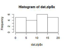
#now for the scatterplot
plot(y~x, dat.zip)
with(subset(dat.zip,y>0), lines(lowess(y~x)))
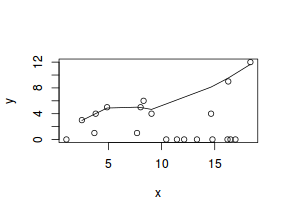
Conclusions: the predictor ($x$) does not display any skewness or other issues that might lead to non-linearity. The lowess smoother on the non-zero data cloud does not display major deviations from a straight line and thus linearity is likely to be satisfied. Violations of linearity (whilst difficult to be certain about due to the unknown influence of the zeros) could be addressed by either:
- define a non-linear linear predictor (such as a polynomial, spline or other non-linear function)
- transform the scale of the predictor variables
Explore zero inflation
Although we have already established that there are few zeros in the data (and thus overdispersion is unlikely to be an issue), we can also explore this by comparing the number of zeros in the data to the number of zeros that would be expected from a Poisson distribution with a mean equal to the mean count of the data.
#proportion of 0's in the data
dat.zip.tab<-table(dat.zip$y==0)
dat.zip.tab/sum(dat.zip.tab)
FALSE  TRUE
 0.55  0.45
#proportion of 0's expected from a Poisson distribution
mu <- mean(dat.zip$y)
cnts <- rpois(1000, mu)
dat.zip.tabE <- table(cnts == 0)
dat.zip.tabE/sum(dat.zip.tabE)
FALSE  TRUE
0.921 0.079
45%) far
exceeds that that would have been expected (7.9%).
Hence it is highly likely that any models will be zero-inflated.
Model fitting or statistical analysis
The exploratory data analyses have suggested that a zero-inflated Poisson model might be the most appropriate for these data.
dat.zip.list <- with(dat.zip,list(Y=y, X=x,N=nrow(dat.zip)))
modelString="
model {
  for (i in 1:N) {
     Y[i] ~ dpois(lambda[i])
     eta[i] <- beta0 + beta1*X[i]
     log(lambda[i]) <- eta[i]
  }
  beta0 ~ dnorm(0,1.0E-06)
  beta1 ~ dnorm(0,1.0E-06)
}
"
writeLines(modelString,con='../downloads/BUGSscripts/tut11.5bS5.4.bug')
library(R2jags)
system.time(
dat.zip.P.jags <- jags(model='../downloads/BUGSscripts/tut11.5bS5.4.bug', data=dat.zip.list, inits=NULL,
          param=c('beta0','beta1'),
          n.chain=3,
          n.iter=20000, n.thin=10, n.burnin=10000)
  )
Compiling model graph
   Resolving undeclared variables
   Allocating nodes
   Graph Size: 105

Initializing model
   user  system elapsed
  1.476   0.000   1.477
print(dat.zip.P.jags)
Inference for Bugs model at "../downloads/BUGSscripts/tut11.5bS5.4.bug", fit using jags,
 3 chains, each with 20000 iterations (first 10000 discarded), n.thin = 10
 n.sims = 3000 iterations saved
         mu.vect sd.vect    2.5%     25%     50%     75%   97.5%  Rhat n.eff
beta0      0.635   0.326  -0.061   0.431   0.644   0.857   1.250 1.001  2400
beta1      0.032   0.025  -0.018   0.014   0.031   0.048   0.084 1.001  2800
deviance 121.928   2.039 120.059 120.548 121.311 122.606 127.122 1.001  3000

For each parameter, n.eff is a crude measure of effective sample size,
and Rhat is the potential scale reduction factor (at convergence, Rhat=1).

DIC info (using the rule, pD = var(deviance)/2)
pD = 2.1 and DIC = 124.0
DIC is an estimate of expected predictive error (lower deviance is better).
#extract the samples for the two model parameters
coefs <- dat.zip.P.jags$BUGSoutput$sims.matrix[,1:2]
Xmat <- model.matrix(~x, data=dat)
#expected values on a log scale
eta<-coefs %*% t(Xmat)
#expected value on response scale
lambda <- exp(eta)

Resid <- -1*sweep(lambda,2,dat.zip$y, '-')/sqrt(lambda)
RSS <- apply(Resid^2, 1, sum)
Disp <- RSS/(nrow(dat.zip)-ncol(coefs))
data.frame(Median=median(Disp), Mean=mean(Disp), HPDinterval(as.mcmc(Disp)), HPDinterval(as.mcmc(Disp),p=0.5))
     Median  Mean lower upper lower.1 upper.1
var1  4.195 4.325 3.181 5.642   3.605   4.426
The dispersion parameter was 4.3250848, indicating over three times more variability than would be expected for a Poisson distribution.
The data are thus over-dispersed. Given the large number of zeros in the response, it would seem likely that the overdispersion is as a result of the
excessive zeros and thus zero-inflated Poisson model would seem reasonable. Note, if this model is still overdispersed (possibly due to clumpiness
in the non-zero values), then a zero-inflated negative binomial model might be worth exploring.
JAGS
$$ Y_i = \left\{ \begin{array}{lrcl} 0~\text{with}~P(y_i) = 1-\mu & z_i&\sim&\text{Binom}(1-\theta)\\ & logit(\theta)&=&\gamma_0\\ &\gamma_0&\sim{}&\mathcal{N}(0,10000)\\ >0 & Y_i&\sim&\text{Pois}(\lambda_i)\\ &\lambda_i&=&z_i + \eta_i\\ &log(\eta_i)&=&\beta_0+\beta_1x_1\\ &\beta_0, \beta_1&\sim{}&\mathcal{N}(0,10000)\\ \end{array} \right. $$ Or in shorthand: $$ \begin{align} Y_i&\sim{}ZIP(\lambda,\theta) & (\text{response distribution})\\ logit(\theta)&=\gamma_0 & (\text{link function/linear predictor - zero component})\\ log(\lambda_i)&=\eta_i & (\text{link function - count component})\\ \eta_i&=\beta_0+\beta_1 X_i & (\text{linear predictor - count component})\\ \beta_0, \beta_1, \gamma_0&\sim{}\mathcal{N}(0,10000) & (\text{diffuse Bayesian priors})\\ \end{align} $$dat.zip.list <- with(dat.zip,list(Y=y, X=x,N=nrow(dat.nb), z=ifelse(y==0,0,1))) modelString=" model { for (i in 1:N) { z[i] ~ dbern(one.minus.theta) Y[i] ~ dpois(lambda[i]) lambda[i] <- z[i]*eta[i] log(eta[i]) <- beta0 + beta1*X[i] } one.minus.theta <- 1-theta logit(theta) <- gamma0 beta0 ~ dnorm(0,1.0E-06) beta1 ~ dnorm(0,1.0E-06) gamma0 ~ dnorm(0,1.0E-06) } " writeLines(modelString,con='../downloads/BUGSscripts/tut11.5bS5.5.bug') library(R2jags) system.time( dat.zip.jags <- jags(model='../downloads/BUGSscripts/tut11.5bS5.5.bug', data=dat.zip.list, inits=NULL, param=c('beta0','beta1', 'gamma0','theta'), n.chain=3, n.iter=20000, n.thin=10, n.burnin=10000) )
Compiling model graph
   Resolving undeclared variables
   Allocating nodes
   Graph Size: 149

Initializing model
   user  system elapsed
  2.492   0.004   2.503
Xmat <- model.matrix(~x, dat.zip)
nX <- ncol(Xmat)
dat.zip.list1 <- with(dat.zip,list(Y=y, X=Xmat,N=nrow(dat.zip), nX=nX, z=ifelse(y==0,0,1)))
modelString="
model {
  for (i in 1:N) {
     z[i] ~ dbern(one.minus.theta)
     Y[i] ~ dpois(lambda[i])
     lambda[i] <- z[i]*eta[i]
     log(eta[i]) <- inprod(beta[], X[i,])
  }
  one.minus.theta <- 1-theta
  logit(theta) <- gamma0
  gamma0 ~ dnorm(0,1.0E-06)
  for (i in 1:nX) {
    beta[i] ~ dnorm(0,1.0E-06)
  }
}
"
writeLines(modelString,con='../downloads/BUGSscripts/tut11.5bS5.6.bug')
library(R2jags)
system.time(
dat.zip.jags1 <- jags(model='../downloads/BUGSscripts/tut11.5bS5.6.bug', data=dat.zip.list1, inits=NULL,
          param=c('beta','gamma0'),
          n.chain=3,
          n.iter=20000, n.thin=10, n.burnin=10000)
  )
Compiling model graph
   Resolving undeclared variables
   Allocating nodes
   Graph Size: 171

Initializing model
   user  system elapsed
  2.465   0.004   2.470
print(dat.zip.jags1)
Inference for Bugs model at "../downloads/BUGSscripts/tut11.5bS5.6.bug", fit using jags,
 3 chains, each with 20000 iterations (first 10000 discarded), n.thin = 10
 n.sims = 3000 iterations saved
         mu.vect sd.vect   2.5%    25%    50%    75%  97.5%  Rhat n.eff
beta[1]    0.709   0.316  0.059  0.495  0.723  0.922  1.304 1.001  3000
beta[2]    0.086   0.025  0.039  0.070  0.085  0.103  0.135 1.001  3000
gamma0    -0.197   0.462 -1.097 -0.508 -0.198  0.113  0.724 1.001  3000
deviance  75.675   2.578 72.834 73.815 74.979 76.794 82.470 1.001  3000

For each parameter, n.eff is a crude measure of effective sample size,
and Rhat is the potential scale reduction factor (at convergence, Rhat=1).

DIC info (using the rule, pD = var(deviance)/2)
pD = 3.3 and DIC = 79.0
DIC is an estimate of expected predictive error (lower deviance is better).
Or arguably better still, use a multivariate normal prior. If we have a $k$ regression parameters ($\beta_k$), then the multivariate normal priors are defined as: $$ \boldsymbol{\beta}\sim{}\mathcal{N_k}(\boldsymbol{\mu}, \mathbf{\Sigma}) $$ where $$\boldsymbol{\mu}=[E[\beta_1],E[\beta_2],...,E[\beta_k]] = \left(\begin{array}{c}0\\\vdots\\0\end{array}\right)$$ $$ \mathbf{\Sigma}=[Cov[\beta_i, \beta_j]] = \left(\begin{array}{ccc}1000^2&0&0\\0&\ddots&0\\0&0&1000^2\end{array} \right) $$ hence, along with the response and predictor matrix, we need to supply $\boldsymbol{\mu}$ (a vector of zeros) and $\boldsymbol{\Sigma}$ (a covariance matrix with $1000^2$ in the diagonals).
Xmat <- model.matrix(~x, dat.zip)
nX <- ncol(Xmat)
dat.zip.list2 <- with(dat.zip,list(Y=y, X=Xmat,N=nrow(dat.zip), nX=nX,
                      mu=rep(0,nX),Sigma=diag(1.0E-06,nX), z=ifelse(y==0,0,1)))
modelString="
model {
  for (i in 1:N) {
     z[i] ~ dbern(one.minus.theta)
     Y[i] ~ dpois(lambda[i])
     lambda[i] <- z[i]*eta[i]
     log(eta[i]) <- inprod(beta[], X[i,])
  }
  one.minus.theta <- 1-theta
  logit(theta) <- gamma0
  gamma0 ~ dnorm(0,1.0E-06)
  beta ~ dmnorm(mu[],Sigma[,])
}
"
writeLines(modelString,con='../downloads/BUGSscripts/tut11.5bS5.7.bug')
library(R2jags)
system.time(
dat.zip.jags2 <- jags(model='../downloads/BUGSscripts/tut11.5bS5.7.bug', data=dat.zip.list2, inits=NULL,
          param=c('beta', 'gamma0'),
          n.chain=3,
          n.iter=20000, n.thin=10, n.burnin=10000)
  )
Compiling model graph
   Resolving undeclared variables
   Allocating nodes
   Graph Size: 176

Initializing model
   user  system elapsed
  0.912   0.004   0.923
print(dat.zip.jags2)
Inference for Bugs model at "../downloads/BUGSscripts/tut11.5bS5.7.bug", fit using jags,
 3 chains, each with 20000 iterations (first 10000 discarded), n.thin = 10
 n.sims = 3000 iterations saved
         mu.vect sd.vect   2.5%    25%    50%    75%  97.5%  Rhat n.eff
beta[1]    0.700   0.321  0.054  0.484  0.702  0.924  1.301 1.001  3000
beta[2]    0.087   0.025  0.038  0.070  0.087  0.104  0.136 1.001  3000
gamma0    -0.217   0.462 -1.155 -0.524 -0.201  0.094  0.674 1.001  3000
deviance  75.688   2.477 72.857 73.895 75.026 76.816 82.064 1.002  2400

For each parameter, n.eff is a crude measure of effective sample size,
and Rhat is the potential scale reduction factor (at convergence, Rhat=1).

DIC info (using the rule, pD = var(deviance)/2)
pD = 3.1 and DIC = 78.8
DIC is an estimate of expected predictive error (lower deviance is better).
Note, the n.eff indicates that we probably have an issue with chain mixing and/or autocorrelation. We probably should increase the number of iterations and the thinning rate.
dat.zip.brm <- brm(y~0+spec + main + main:x, data=dat.zip, family='zero_inflated_poisson',
  prior = c(set_prior("normal(0,100)", class="b")),
  chains=3, iter=2000, warmup=1000, thin=2)
SAMPLING FOR MODEL 'zero_inflated_poisson(log) brms-model' NOW (CHAIN 1).

Chain 1, Iteration:    1 / 2000 [  0%]  (Warmup)
Chain 1, Iteration:  200 / 2000 [ 10%]  (Warmup)
Chain 1, Iteration:  400 / 2000 [ 20%]  (Warmup)
Chain 1, Iteration:  600 / 2000 [ 30%]  (Warmup)
Chain 1, Iteration:  800 / 2000 [ 40%]  (Warmup)
Chain 1, Iteration: 1000 / 2000 [ 50%]  (Warmup)
Chain 1, Iteration: 1001 / 2000 [ 50%]  (Sampling)
Chain 1, Iteration: 1200 / 2000 [ 60%]  (Sampling)
Chain 1, Iteration: 1400 / 2000 [ 70%]  (Sampling)
Chain 1, Iteration: 1600 / 2000 [ 80%]  (Sampling)
Chain 1, Iteration: 1800 / 2000 [ 90%]  (Sampling)
Chain 1, Iteration: 2000 / 2000 [100%]  (Sampling)#
#  Elapsed Time: 0.184441 seconds (Warm-up)
#                0.109929 seconds (Sampling)
#                0.29437 seconds (Total)
#

SAMPLING FOR MODEL 'zero_inflated_poisson(log) brms-model' NOW (CHAIN 2).

Chain 2, Iteration:    1 / 2000 [  0%]  (Warmup)
Chain 2, Iteration:  200 / 2000 [ 10%]  (Warmup)
Chain 2, Iteration:  400 / 2000 [ 20%]  (Warmup)
Chain 2, Iteration:  600 / 2000 [ 30%]  (Warmup)
Chain 2, Iteration:  800 / 2000 [ 40%]  (Warmup)
Chain 2, Iteration: 1000 / 2000 [ 50%]  (Warmup)
Chain 2, Iteration: 1001 / 2000 [ 50%]  (Sampling)
Chain 2, Iteration: 1200 / 2000 [ 60%]  (Sampling)
Chain 2, Iteration: 1400 / 2000 [ 70%]  (Sampling)
Chain 2, Iteration: 1600 / 2000 [ 80%]  (Sampling)
Chain 2, Iteration: 1800 / 2000 [ 90%]  (Sampling)
Chain 2, Iteration: 2000 / 2000 [100%]  (Sampling)#
#  Elapsed Time: 0.18517 seconds (Warm-up)
#                0.121613 seconds (Sampling)
#                0.306783 seconds (Total)
#

SAMPLING FOR MODEL 'zero_inflated_poisson(log) brms-model' NOW (CHAIN 3).

Chain 3, Iteration:    1 / 2000 [  0%]  (Warmup)
Chain 3, Iteration:  200 / 2000 [ 10%]  (Warmup)
Chain 3, Iteration:  400 / 2000 [ 20%]  (Warmup)
Chain 3, Iteration:  600 / 2000 [ 30%]  (Warmup)
Chain 3, Iteration:  800 / 2000 [ 40%]  (Warmup)
Chain 3, Iteration: 1000 / 2000 [ 50%]  (Warmup)
Chain 3, Iteration: 1001 / 2000 [ 50%]  (Sampling)
Chain 3, Iteration: 1200 / 2000 [ 60%]  (Sampling)
Chain 3, Iteration: 1400 / 2000 [ 70%]  (Sampling)
Chain 3, Iteration: 1600 / 2000 [ 80%]  (Sampling)
Chain 3, Iteration: 1800 / 2000 [ 90%]  (Sampling)
Chain 3, Iteration: 2000 / 2000 [100%]  (Sampling)#
#  Elapsed Time: 0.183662 seconds (Warm-up)
#                0.125256 seconds (Sampling)
#                0.308918 seconds (Total)
#
## Or if we allow the zero-inflation model and the count model to vary with x
dat.zip.brm1 <- brm(y~trait:x, data=dat.zip, family='zero_inflated_poisson',
  prior = c(set_prior("normal(0,100)", class="b")),
  chains=3, iter=2000, warmup=1000, thin=2)
SAMPLING FOR MODEL 'zero_inflated_poisson(log) brms-model' NOW (CHAIN 1).

Chain 1, Iteration:    1 / 2000 [  0%]  (Warmup)
Chain 1, Iteration:  200 / 2000 [ 10%]  (Warmup)
Chain 1, Iteration:  400 / 2000 [ 20%]  (Warmup)
Chain 1, Iteration:  600 / 2000 [ 30%]  (Warmup)
Chain 1, Iteration:  800 / 2000 [ 40%]  (Warmup)
Chain 1, Iteration: 1000 / 2000 [ 50%]  (Warmup)
Chain 1, Iteration: 1001 / 2000 [ 50%]  (Sampling)
Chain 1, Iteration: 1200 / 2000 [ 60%]  (Sampling)
Chain 1, Iteration: 1400 / 2000 [ 70%]  (Sampling)
Chain 1, Iteration: 1600 / 2000 [ 80%]  (Sampling)
Chain 1, Iteration: 1800 / 2000 [ 90%]  (Sampling)
Chain 1, Iteration: 2000 / 2000 [100%]  (Sampling)#
#  Elapsed Time: 0.140589 seconds (Warm-up)
#                0.212475 seconds (Sampling)
#                0.353064 seconds (Total)
#

SAMPLING FOR MODEL 'zero_inflated_poisson(log) brms-model' NOW (CHAIN 2).

Chain 2, Iteration:    1 / 2000 [  0%]  (Warmup)
Chain 2, Iteration:  200 / 2000 [ 10%]  (Warmup)
Chain 2, Iteration:  400 / 2000 [ 20%]  (Warmup)
Chain 2, Iteration:  600 / 2000 [ 30%]  (Warmup)
Chain 2, Iteration:  800 / 2000 [ 40%]  (Warmup)
Chain 2, Iteration: 1000 / 2000 [ 50%]  (Warmup)
Chain 2, Iteration: 1001 / 2000 [ 50%]  (Sampling)
Chain 2, Iteration: 1200 / 2000 [ 60%]  (Sampling)
Chain 2, Iteration: 1400 / 2000 [ 70%]  (Sampling)
Chain 2, Iteration: 1600 / 2000 [ 80%]  (Sampling)
Chain 2, Iteration: 1800 / 2000 [ 90%]  (Sampling)
Chain 2, Iteration: 2000 / 2000 [100%]  (Sampling)#
#  Elapsed Time: 0.154223 seconds (Warm-up)
#                0.130932 seconds (Sampling)
#                0.285155 seconds (Total)
#

SAMPLING FOR MODEL 'zero_inflated_poisson(log) brms-model' NOW (CHAIN 3).

Chain 3, Iteration:    1 / 2000 [  0%]  (Warmup)
Chain 3, Iteration:  200 / 2000 [ 10%]  (Warmup)
Chain 3, Iteration:  400 / 2000 [ 20%]  (Warmup)
Chain 3, Iteration:  600 / 2000 [ 30%]  (Warmup)
Chain 3, Iteration:  800 / 2000 [ 40%]  (Warmup)
Chain 3, Iteration: 1000 / 2000 [ 50%]  (Warmup)
Chain 3, Iteration: 1001 / 2000 [ 50%]  (Sampling)
Chain 3, Iteration: 1200 / 2000 [ 60%]  (Sampling)
Chain 3, Iteration: 1400 / 2000 [ 70%]  (Sampling)
Chain 3, Iteration: 1600 / 2000 [ 80%]  (Sampling)
Chain 3, Iteration: 1800 / 2000 [ 90%]  (Sampling)
Chain 3, Iteration: 2000 / 2000 [100%]  (Sampling)#
#  Elapsed Time: 0.139585 seconds (Warm-up)
#                0.132922 seconds (Sampling)
#                0.272507 seconds (Total)
#
Chain mixing and Model validation
Prior to exploring the model parameters, it is prudent to confirm that the model did indeed fit the assumptions and was an appropriate fit to the data as well as that the MCMC sampling chain was adequately mixed and the retained samples independent.
- We will start by exploring the mixing of the MCMC chains via traceplots.
plot(as.mcmc(dat.zip.jags))
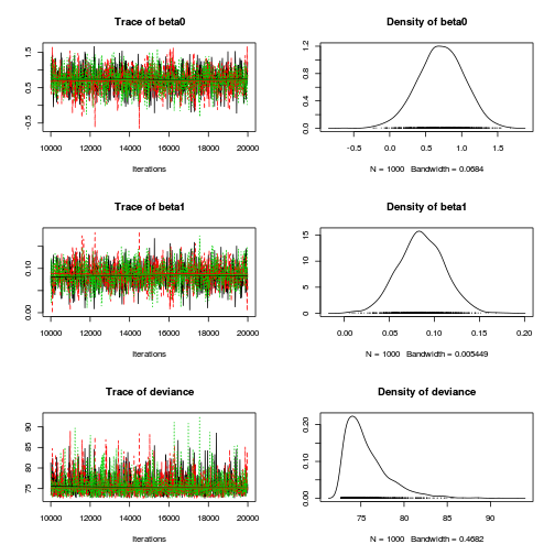
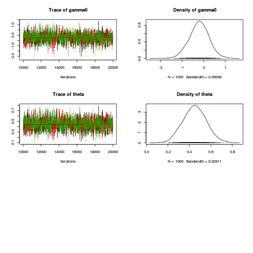
The chains appear well mixed and stable
library(gridExtra)
grid.arrange(stan_trace(dat.zip.brm$fit, ncol=1),
             stan_dens(dat.zip.brm$fit, separate_chains=TRUE,ncol=1),
             ncol=2)
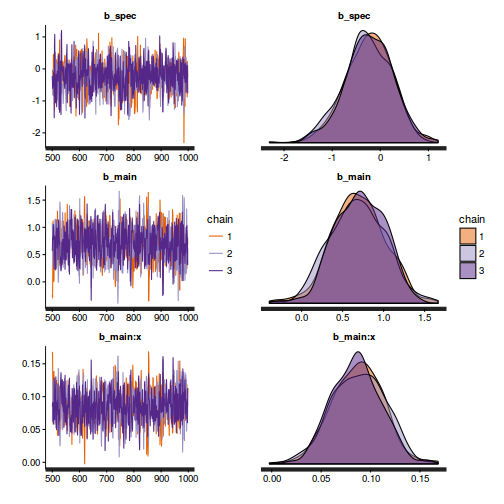
- Next we will explore correlation amongst MCMC samples.
autocorr.diag(as.mcmc(dat.zip.jags))
            beta0      beta1  deviance     gamma0     theta
Lag 0    1.000000  1.0000000  1.000000  1.0000000  1.000000
Lag 10   0.275638  0.2908784  0.043162  0.0469457  0.048194
Lag 50  -0.006762  0.0226283 -0.007629  0.0035146  0.002608
Lag 100  0.016017  0.0046681 -0.008336  0.0003516 -0.000948
Lag 500 -0.001439 -0.0009426 -0.003084 -0.0085311 -0.010254
The level of auto-correlation at the nominated lag of 10 is higher than we would generally like. It is worth increasing the thinning rate from 10 to 50. Obviously, to support this higher thinning rate, we would also increase the number of iterations.
library(R2jags)
dat.zip.jags <- jags(data=dat.zip.list,model.file='../downloads/BUGSscripts/tut11.5bS5.5.bug',
                   param=c('beta0','beta1','gamma0','theta'),
                   n.chains=3, n.iter=100000, n.burnin=50000, n.thin=50)
Compiling model graph
   Resolving undeclared variables
   Allocating nodes
   Graph Size: 149

Initializing model
print(dat.zip.jags)
Inference for Bugs model at "../downloads/BUGSscripts/tut11.5bS5.5.bug", fit using jags, 3 chains, each with 1e+05 iterations (first 50000 discarded), n.thin = 50 n.sims = 3000 iterations saved mu.vect sd.vect 2.5% 25% 50% 75% 97.5% Rhat n.eff beta0 0.706 0.319 0.043 0.494 0.716 0.928 1.301 1.001 2800 beta1 0.086 0.026 0.037 0.069 0.086 0.103 0.137 1.001 2300 gamma0 -0.220 0.466 -1.127 -0.541 -0.212 0.107 0.670 1.002 1800 theta 0.448 0.110 0.245 0.368 0.447 0.527 0.661 1.001 2000 deviance 75.685 2.453 72.827 73.883 75.054 76.878 81.846 1.001 2300 For each parameter, n.eff is a crude measure of effective sample size, and Rhat is the potential scale reduction factor (at convergence, Rhat=1). DIC info (using the rule, pD = var(deviance)/2) pD = 3.0 and DIC = 78.7 DIC is an estimate of expected predictive error (lower deviance is better).plot(as.mcmc(dat.zip.jags))
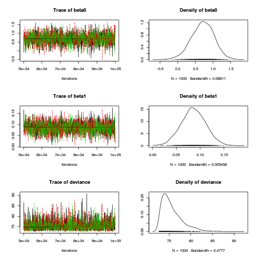
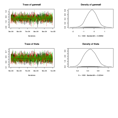
autocorr.diag(as.mcmc(dat.zip.jags))
             beta0     beta1  deviance    gamma0     theta
Lag 0     1.000000  1.000000  1.000000  1.000000  1.000000
Lag 50   -0.003957 -0.029631  0.016977 -0.019662 -0.019085
Lag 250   0.020470  0.011623 -0.016871  0.009786  0.011709
Lag 500   0.010446  0.003702  0.003925 -0.048037 -0.047746
Lag 2500 -0.026443  0.002784 -0.021067 -0.005668 -0.003888
Conclusions: the samples are now less auto-correlated and the chains are all well mixed and appear stable.
stan_ac(dat.zip.brm$fit)
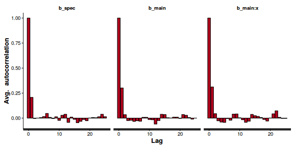
- Explore the step size characteristics (STAN only)
Conclusions: acceptance ratio is very good, the lot posterior is relatively robust to step size and tree depth, rhat values are all below 1.05, the effective sample size is not too bad (we might be able to achieve better acceptance ratios with tighter priors) and the ratio of MCMC error to posterior sd is very small.
summary(do.call(rbind, args = get_sampler_params(dat.zip.brm$fit, inc_warmup = FALSE)), digits = 2)
 accept_stat__    stepsize__    treedepth__   n_leapfrog__  n_divergent__
 Min.   :0.19   Min.   :0.29   Min.   :1.0   Min.   : 1.0   Min.   :0
 1st Qu.:0.89   1st Qu.:0.29   1st Qu.:2.0   1st Qu.: 3.0   1st Qu.:0
 Median :0.96   Median :0.35   Median :3.0   Median : 7.0   Median :0
 Mean   :0.92   Mean   :0.33   Mean   :2.9   Mean   : 7.6   Mean   :0
 3rd Qu.:0.99   3rd Qu.:0.36   3rd Qu.:4.0   3rd Qu.:11.0   3rd Qu.:0
 Max.   :1.00   Max.   :0.36   Max.   :4.0   Max.   :15.0   Max.   :0
stan_diag(dat.zip.brm$fit)
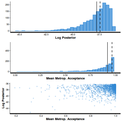
stan_diag(dat.zip.brm$fit, information = "stepsize")
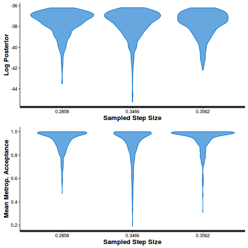
stan_diag(dat.zip.brm$fit, information = "treedepth")
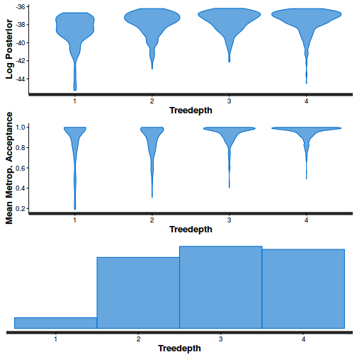
stan_diag(dat.zip.brm$fit, information = "divergence")
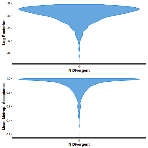
library(gridExtra)
grid.arrange(stan_rhat(dat.zip.brm$fit) + theme_classic(8),
             stan_ess(dat.zip.brm$fit) + theme_classic(8),
             stan_mcse(dat.zip.brm$fit) + theme_classic(8),
             ncol = 2)
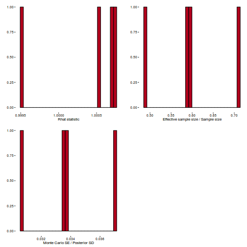
- We now explore the goodness of fit of the models via the residuals and deviance.
We could calculate the Pearsons's residuals within the JAGS model.
Alternatively, we could use the parameters to generate the residuals outside of JAGS.
#extract the samples for the two model parameters
coefs <- dat.zip.jags$BUGSoutput$sims.matrix[,1:2]
theta <- dat.zip.jags$BUGSoutput$sims.matrix[,'theta']
Xmat <- model.matrix(~x, data=dat.zip)
#expected values on a log scale
lambda<-coefs %*% t(Xmat)
#expected value on response scale
eta <- exp(lambda)
expY <- sweep(eta,1,(1-theta),"*")
varY <- eta+sweep(eta^2,1,theta,"*")
varY <- sweep(varY,1,(1-theta),'*')
#sweep across rows and then divide by lambda
Resid <- -1*sweep(expY,2,dat.zip$y,'-')/sqrt(varY)
#plot residuals vs expected values
plot(apply(Resid,2,mean)~apply(eta,2,mean))
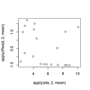
#Calculate residuals
Resid.zip.brm <- residuals(dat.zip.brm, type='pearson')[,'Estimate']
#Extract the fitted values.  Note, since a zero-inflated model is really two models
#(the binary process and the poisson process), there are fitted values associated
#with both processes.  The first half of the fitted values are associated with
#the count process (the ones we are interested in here), the second half are
#associated with the binomial process.
#Furthermore, dont be tempted to use fitted(dat.zip.brm, scale='response',...) with
#zero inflated models, they seem to be a bit odd...
Fitted.zip.brm <- exp(fitted(dat.zip.brm, scale='linear')[1:nrow(dat.zip),'Estimate'])
ggplot(data=NULL, aes(y=Resid.zip.brm, x=Fitted.zip.brm)) + geom_point()
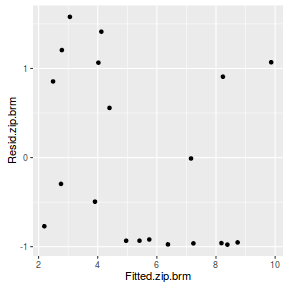
## Or the x varying zero-inflated and count model
Resid.zip.brm <- residuals(dat.zip.brm1, type='pearson')[,'Estimate']
Fitted.zip.brm <- exp(fitted(dat.zip.brm1, scale='linear')[1:nrow(dat.zip),'Estimate'])
ggplot(data=NULL, aes(y=Resid.zip.brm, x=Fitted.zip.brm)) + geom_point()
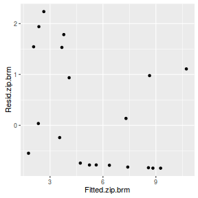
There are no real patterns in the residuals.
- Now we will compare the sum of squared residuals to the sum of squares residuals that would be expected from a Poisson distribution
matching that estimated by the model. Essentially this is estimating how well the Poisson distribution, the log-link function and the linear model
approximates the observed data.
When doing so, we need to consider the expected value and variance of the zero-inflated poisson. $$ E(y_i) = \lambda\times(1-\theta)\\ Var(y_i) = \lambda\times(1-\theta)\times(1+\theta\times\lambda^2) $$
SSres<-apply(Resid^2,1,sum)

set.seed(2)
#generate a matrix of draws from a zero-inflated poisson (ZIP) distribution
# the matrix is the same dimensions as lambda
library(gamlss.dist)
#YNew <- matrix(rZIP(length(lambda),eta, theta),nrow=nrow(lambda))
lambda <- sweep(eta,1,ifelse(dat.zip$y==0,0,1),'*')
YNew <- matrix(rpois(length(lambda),lambda),nrow=nrow(lambda))
Resid1<-(expY - YNew)/sqrt(varY)
SSres.sim<-apply(Resid1^2,1,sum)
mean(SSres.sim>SSres)
[1] 0.4346667
Whilst not ideal (as we would prefer a Bayesian P-value of around 0.5), this value is not wildly bad and does not constitute overwhelming evidence of a lack of fit.
Xmat <- model.matrix(~x, dat.zip)
nX <- ncol(Xmat)
dat.zip.list2 <- with(dat.zip,list(Y=y, X=Xmat,N=nrow(dat.zip), nX=nX,
                      mu=rep(0,nX),Sigma=diag(1.0E-06,nX), z=ifelse(y==0,0,1)))
modelString="
model {
  for (i in 1:N) {
     z[i] ~ dbern(one.minus.theta)
     Y[i] ~ dpois(lambda[i])
     lambda[i] <- z[i]*eta[i]
     log(eta[i]) <- max(-20,min(20,inprod(beta[], X[i,])))

     expY[i] <- eta[i]*(1-theta)
     varY[i] <- (1-theta)*(eta[i]*theta*pow(eta[i],2))
     Resid[i] <- (Y[i] - expY[i])/sqrt(varY[i])
     Y1[i] ~ dpois(lambda[i])
     Resid1[i] <- (Y1[i] - expY[i])/sqrt(varY[i])
     RSS[i] <- pow(Resid[i],2)
     RSS1[i] <-pow(Resid1[i],2)
  }
  one.minus.theta <- 1-theta
  logit(theta) <- gamma0
  gamma0 ~ dnorm(0,1.0E-06)
  beta ~ dmnorm(mu[],Sigma[,])
  Pvalue <- mean(sum(RSS1)>sum(RSS))
}
"
writeLines(modelString,con='../downloads/BUGSscripts/tut11.5bS5.13.bug')
library(R2jags)
system.time(
dat.zip.jags3 <- jags(model='../downloads/BUGSscripts/tut11.5bS5.13.bug', data=dat.zip.list2, inits=NULL,
          param=c('beta', 'gamma0','Pvalue'),
          n.chain=3,
          n.iter=20000, n.thin=10, n.burnin=10000)
  )
Compiling model graph
   Resolving undeclared variables
   Allocating nodes
   Graph Size: 465

Initializing model
   user  system elapsed
  1.321   0.004   1.328
print(dat.zip.jags3)
Inference for Bugs model at "../downloads/BUGSscripts/tut11.5bS5.13.bug", fit using jags, 3 chains, each with 20000 iterations (first 10000 discarded), n.thin = 10 n.sims = 3000 iterations saved mu.vect sd.vect 2.5% 25% 50% 75% 97.5% Rhat n.eff Pvalue 0.455 0.498 0.000 0.000 0.000 1.000 1.000 1.001 3000 beta[1] 0.718 0.320 0.079 0.512 0.729 0.921 1.328 1.001 3000 beta[2] 0.085 0.025 0.034 0.069 0.085 0.101 0.136 1.001 3000 gamma0 -0.197 0.465 -1.096 -0.512 -0.195 0.122 0.711 1.002 1600 deviance 75.686 2.594 72.853 73.845 74.987 76.779 82.738 1.006 1500 For each parameter, n.eff is a crude measure of effective sample size, and Rhat is the potential scale reduction factor (at convergence, Rhat=1). DIC info (using the rule, pD = var(deviance)/2) pD = 3.4 and DIC = 79.0 DIC is an estimate of expected predictive error (lower deviance is better).Resid.zip.brm <- residuals(dat.zip.brm, type='pearson', summary=FALSE) SSres.zip.brm <- apply(Resid.zip.brm^2,1,sum) lambda.zip.brm = fitted(dat.brm, scale='response', summary=FALSE) YNew.zip.brm <- matrix(rpois(length(lambda.zip.brm), lambda=lambda.zip.brm), nrow=nrow(lambda.zip.brm)) Resid1.zip.brm<-(lambda.zip.brm - YNew.zip.brm)/sqrt(lambda.zip.brm) SSres.sim.zip.brm<-apply(Resid1.zip.brm^2,1,sum) mean(SSres.sim.zip.brm>SSres.zip.brm)
[1] 0.482
Conclusions: the Bayesian p-value is very close to 0.5, suggesting that there is a good fit of the model to the data.
- Since it is difficult to diagnose many issues from the typical residuals we will now explore simulated residuals.
The trend (black symbols) in the qq-plot does not appear to be overly non-linear (matching the ideal red line well), suggesting that the model is not overdispersed. The spread of standardized (simulated) residuals in the residual plot do not appear overly non-uniform. That is there is not trend in the residuals. Furthermore, there is not a concentration of points close to 1 or 0 (which would imply overdispersion). Hence, once zero-inflation is accounted for, the model does not display overdispersion.#extract the samples for the two model parameters coefs <- dat.zip.jags$BUGSoutput$sims.matrix[,1:2] theta <- dat.zip.jags$BUGSoutput$sims.matrix[,'theta'] Xmat <- model.matrix(~x, data=dat.zip) #expected values on a log scale eta<-coefs %*% t(Xmat) #expected value on response scale lambda <- exp(eta) simRes <- function(lambda, data,n=250, plot=T, family='negbin', size=NULL,theta=NULL) { require(gap) N = nrow(data) sim = switch(family, 'poisson' = matrix(rpois(n*N,apply(lambda,2,mean)),ncol=N, byrow=TRUE), 'negbin' = matrix(MASS:::rnegbin(n*N,apply(lambda,2,mean),size),ncol=N, byrow=TRUE), 'zip' = matrix(gamlss.dist:::rZIP(n*N,apply(lambda,2,mean),theta),ncol=N, byrow=TRUE) ) a = apply(sim + runif(n,-0.5,0.5),2,ecdf) resid<-NULL for (i in 1:nrow(data)) resid<-c(resid,a[[i]](data$y[i] + runif(1 ,-0.5,0.5))) if (plot==T) { par(mfrow=c(1,2)) gap::qqunif(resid,pch = 2, bty = "n", logscale = F, col = "black", cex = 0.6, main = "QQ plot residuals", cex.main = 1, las=1) plot(resid~apply(lambda,2,mean), xlab='Predicted value', ylab='Standardized residual', las=1) } resid } simRes(lambda,dat.zip, family='zip',theta=theta)
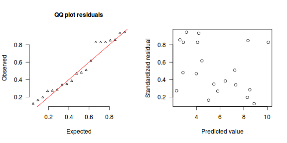
[1] 0.272 0.856 0.480 0.828 0.944 0.468 0.828 0.932 0.616 0.164 0.348 0.268 0.384 0.508 0.340 0.196 0.848 0.284 0.124 0.828
Although there is a slight hint of non-linearity in that the residuals are high for low and high fitted values and lower in the middle, this might well be an artifact of the small data set size. By change, most of the observed values in the middle range of the predictor were zero.
lambda.zip.brm = exp(fitted(dat.zip.brm, scale='linear', summary=FALSE))[,1:nrow(dat.zip)]
theta = binomial()$linkinv(mean(rstan:::extract(dat.zip.brm$fit, 'b_spec')[[1]]))
simRes <- function(lambda, data,n=250, plot=T, family='negbin', size=NULL,theta=NULL) {
 require(gap)
 N = nrow(data)
 sim = switch(family,
    'poisson' = matrix(rpois(n*N,apply(lambda,2,mean)),ncol=N, byrow=TRUE),
    'negbin' = matrix(MASS:::rnegbin(n*N,apply(lambda,2,mean),size),ncol=N, byrow=TRUE),
        'zip' = matrix(gamlss.dist:::rZIP(n*N,apply(lambda,2,mean),theta),ncol=N, byrow=TRUE)
 )
 a = apply(sim + runif(n,-0.5,0.5),2,ecdf)
 resid<-NULL
 for (i in 1:nrow(data)) resid<-c(resid,a[[i]](data$y[i] + runif(1 ,-0.5,0.5)))
 if (plot==T) {
   par(mfrow=c(1,2))
   gap::qqunif(resid,pch = 2, bty = "n",
   logscale = F, col = "black", cex = 0.6, main = "QQ plot residuals",
   cex.main = 1, las=1)
   plot(resid~apply(lambda,2,mean), xlab='Predicted value', ylab='Standardized residual', las=1)
 }
 resid
}

simRes(lambda.zip.brm, dat.zip, family='zip', theta=theta)
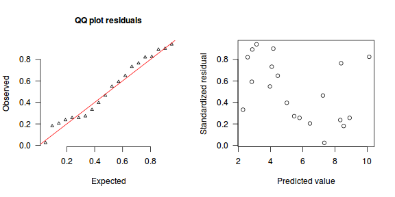
[1] 0.332 0.820 0.592 0.892 0.940 0.548 0.732 0.900 0.648 0.396 0.272 0.256 0.204 0.464 0.024 0.236 0.764 0.180 0.256 0.824
Exploring the model parameters, test hypotheses
If there was any evidence that the assumptions had been violated or the model was not an appropriate fit, then we would need to reconsider the model and start the process again. In this case, there is no evidence that the test will be unreliable so we can proceed to explore the test statistics.
As with most Bayesian models, it is best to base conclusions on medians rather than means.
print(dat.zip.jags)
Inference for Bugs model at "../downloads/BUGSscripts/tut11.5bS5.5.bug", fit using jags, 3 chains, each with 1e+05 iterations (first 50000 discarded), n.thin = 50 n.sims = 3000 iterations saved mu.vect sd.vect 2.5% 25% 50% 75% 97.5% Rhat n.eff beta0 0.706 0.319 0.043 0.494 0.716 0.928 1.301 1.001 2800 beta1 0.086 0.026 0.037 0.069 0.086 0.103 0.137 1.001 2300 gamma0 -0.220 0.466 -1.127 -0.541 -0.212 0.107 0.670 1.002 1800 theta 0.448 0.110 0.245 0.368 0.447 0.527 0.661 1.001 2000 deviance 75.685 2.453 72.827 73.883 75.054 76.878 81.846 1.001 2300 For each parameter, n.eff is a crude measure of effective sample size, and Rhat is the potential scale reduction factor (at convergence, Rhat=1). DIC info (using the rule, pD = var(deviance)/2) pD = 3.0 and DIC = 78.7 DIC is an estimate of expected predictive error (lower deviance is better).library(plyr) adply(dat.zip.jags$BUGSoutput$sims.matrix, 2, function(x) { data.frame(Median=median(x), Mean=mean(x), HPDinterval(as.mcmc(x)), HPDinterval(as.mcmc(x),p=0.5)) })
        X1   Median     Mean    lower   upper  lower.1 upper.1
1    beta0  0.71587  0.70638  0.06835  1.3198  0.57561  0.9971
2    beta1  0.08556  0.08604  0.03607  0.1359  0.07058  0.1042
3 deviance 75.05425 75.68540 72.64080 80.6794 73.02722 75.3436
4   gamma0 -0.21225 -0.21991 -1.14123  0.6553 -0.49398  0.1432
5    theta  0.44714  0.44798  0.24209  0.6582  0.37853  0.5353
Actually, many find it more palatable to express the estimates in the original scale of the observations rather than on a log scale.
library(plyr)
adply(exp(dat.zip.jags$BUGSoutput$sims.matrix[,1:2]), 2, function(x) {
  data.frame(Median=median(x), Mean=mean(x), HPDinterval(as.mcmc(x)), HPDinterval(as.mcmc(x),p=0.5))
})
     X1 Median Mean  lower upper lower.1 upper.1
1 beta0  2.046 2.13 0.9547 3.495   1.536   2.392
2 beta1  1.089 1.09 1.0351 1.144   1.073   1.110
Conclusions: We would reject the null hypothesis of no effect of $x$ on $y$. An increase in x is associated with a significant linear increase (positive slope) in the abundance of $y$. Every 1 unit increase in $x$ results in a log
0.0855612unit increase in $y$. We usually express this in terms of abundance rather than log abundance, so every 1 unit increase in $x$ results in a ($e^{0.0855612}=1.0893282$)1.0893282unit increase in the abundance of $y$.summary(dat.zip.brm)
Family: zero_inflated_poisson (log) Formula: y ~ 0 + spec + main + main:x Data: dat.zip (Number of observations: 20) Samples: 3 chains, each with iter = 2000; warmup = 1000; thin = 2; total post-warmup samples = 1500 WAIC: Not computed Fixed Effects: Estimate Est.Error l-95% CI u-95% CI Eff.Sample Rhat spec -0.25 0.49 -1.27 0.65 1060 1 main 0.70 0.32 0.08 1.30 896 1 main:x 0.09 0.03 0.04 0.13 877 1 Samples were drawn using sampling(NUTS). For each parameter, Eff.Sample is a crude measure of effective sample size, and Rhat is the potential scale reduction factor on split chains (at convergence, Rhat = 1).exp(coef(dat.zip.brm))
            mean
spec   0.7810716
main   2.0043001
main:x 1.0907019
coefs.zip.brm <- as.matrix(as.data.frame(rstan:::extract(dat.zip.brm$fit)))
coefs.zip.brm <- coefs.zip.brm[,grep('b', colnames(coefs.zip.brm))]
plyr:::adply(exp(coefs.zip.brm), 2, function(x) {
  data.frame(Mean=mean(x), median=median(x), HPDinterval(as.mcmc(x)))
  })
X1 Mean median lower upper 1 b_spec 0.8761436 0.7914704 0.2026179 1.690390 2 b_main 2.1094730 2.0088827 0.9788579 3.463095 3 b_main.x 1.0910609 1.0910342 1.0360825 1.141645
marginal_effects(dat.zip.brm)
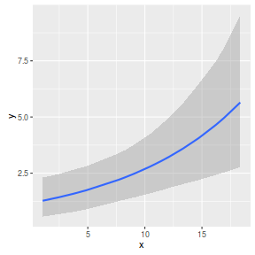
Further explorations of the trends
A measure of the strength of the relationship can be obtained according to: $$R^2 = 1 - \frac{RSS_{model}}{RSS_{null}}$$
Alternatively, we could use McFadden's psuedo $$R^2 = 1-\frac{\mathcal{LL}(Model_{full})}{\mathcal{LL}(Model_{reduced})}$$ [[http://www.statisticalhorizons.com/category/uncategorized]] - about a quarter of the way down the page.
Xmat <- model.matrix(~x, dat=dat.zip) #expected values on a log scale neta<-coefs %*% t(Xmat) #expected value on response scale eta <- exp(neta) lambda <- sweep(eta,2,ifelse(dat.zip$y==0,0,1),'*') theta <- dat.zip.jags$BUGSoutput$sims.matrix[,'theta'] expY <- sweep(lambda,2,1-theta,'*') #calculate the raw SS residuals SSres <- apply((-1*(sweep(expY,2,dat.zip$y,'-')))^2,1,sum) mean(SSres)
[1] 112.5743
SSres.null <- sum((dat.zip$y - mean(dat.zip$y))^2) #calculate the model r2 1-mean(SSres)/SSres.null
[1] 0.4978847
Conclusions:
49.79% of the variation in $y$ abundance can be explained by its relationship with $x$.Xmat <- model.matrix(~x, dat.zip) nX <- ncol(Xmat) dat.zip.list2 <- with(dat.zip,list(Y=y, X=Xmat,N=nrow(dat.zip), nX=nX, mu=rep(0,nX),Sigma=diag(1.0E-06,nX), z=ifelse(y==0,0,1))) modelString=" model { for (i in 1:N) { z[i] ~ dbern(one.minus.theta) Y[i] ~ dpois(lambda[i]) lambda[i] <- z[i]*eta[i] log(eta[i]) <- max(-20,min(20,inprod(beta[], X[i,]))) expY[i] <- lambda[i]*(1-theta) res[i] <- Y[i] - expY[i] resnull[i] <- Y[i] - meanY } one.minus.theta <- 1-theta logit(theta) <- gamma0 gamma0 ~ dnorm(0,1.0E-06) beta ~ dmnorm(mu[],Sigma[,]) meanY <- mean(Y) RSS <- sum(res^2) RSSnull <- sum(resnull^2) r2 <- 1-RSS/RSSnull } " writeLines(modelString,con='../downloads/BUGSscripts/tut11.5bS5.17.bug') library(R2jags) system.time( dat.ZIP.jags4 <- jags(model='../downloads/BUGSscripts/tut11.5bS5.17.bug', data=dat.zip.list2, inits=NULL, param=c('beta','r2'), n.chain=3, n.iter=20000, n.thin=10, n.burnin=10000) )
Compiling model graph Resolving undeclared variables Allocating nodes Graph Size: 277 Initializing model
user system elapsed 1.072 0.000 1.075
print(dat.ZIP.jags4)
Inference for Bugs model at "../downloads/BUGSscripts/tut11.5bS5.17.bug", fit using jags, 3 chains, each with 20000 iterations (first 10000 discarded), n.thin = 10 n.sims = 3000 iterations saved mu.vect sd.vect 2.5% 25% 50% 75% 97.5% Rhat n.eff beta[1] 0.724 0.313 0.064 0.522 0.737 0.941 1.304 1.003 880 beta[2] 0.085 0.025 0.037 0.067 0.084 0.101 0.134 1.002 1200 r2 0.492 0.176 0.113 0.377 0.504 0.622 0.787 1.002 1800 deviance 75.612 2.516 72.833 73.816 74.930 76.635 82.063 1.001 3000 For each parameter, n.eff is a crude measure of effective sample size, and Rhat is the potential scale reduction factor (at convergence, Rhat=1). DIC info (using the rule, pD = var(deviance)/2) pD = 3.2 and DIC = 78.8 DIC is an estimate of expected predictive error (lower deviance is better).Xmat <- model.matrix(~x, dat=dat.zip) #expected values on a log scale coefs.zip <- as.matrix(as.data.frame(rstan:::extract(dat.zip.brm$fit))) coefs.zip <- coefs.zip[,grep('b.main', colnames(coefs.zip))] neta<-coefs.zip %*% t(Xmat) #expected value on response scale eta <- exp(neta) lambda <- sweep(eta,2,ifelse(dat.zip$y==0,0,1),'*') theta <- dat.zip.jags$BUGSoutput$sims.matrix[,'theta'] expY <- sweep(lambda,2,1-theta,'*') #calculate the raw SS residuals SSres <- apply((-1*(sweep(expY,2,dat.zip$y,'-')))^2,1,sum) SSres.null <- sum((dat.zip$y - mean(dat.zip$y))^2) #OR SSres.null <- crossprod(dat.zip$y - mean(dat.zip$y)) #calculate the model r2 1-mean(SSres)/SSres.null
[,1] [1,] 0.497461
Finally, we will create a summary plot.
par(mar = c(4, 5, 0, 0)) plot(y ~ x, data = dat.zip, type = "n", ann = F, axes = F) points(y ~ x, data = dat.zip, pch = 16) xs <- seq(min(dat.zip$x,na.rm=TRUE),max(dat.zip$x,na.rm=TRUE), l = 1000) Xmat <- model.matrix(~xs) eta<-coefs %*% t(Xmat) ys <- exp(eta) library(plyr) library(coda) data.tab <- adply(ys,2,function(x) { data.frame(Median=median(x), HPDinterval(as.mcmc(x))) }) data.tab <- cbind(x=xs,data.tab) points(Median ~ x, data=data.tab,col = "black", type = "l") lines(lower ~ x, data=data.tab,col = "black", type = "l", lty = 2) lines(upper ~ x, data=data.tab,col = "black", type = "l", lty = 2) axis(1) mtext("X", 1, cex = 1.5, line = 3) axis(2, las = 2) mtext("Abundance of Y", 2, cex = 1.5, line = 3) box(bty = "l")
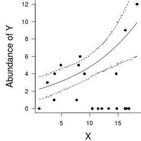
newdata = data.frame(x=seq(min(dat.zip$x), max(dat.zip$x), len=100)) Xmat = model.matrix(~x, data=newdata) coefs <- as.matrix(as.data.frame(rstan:::extract(dat.zip.brm$fit))) coefs <- coefs[,grep('b_main', colnames(coefs))] fit = exp(coefs %*% t(Xmat)) newdata = cbind(newdata, plyr:::adply(fit, 2, function(x) { data.frame(Mean=mean(x), Median=median(x), HPDinterval(as.mcmc(x))) }) ) ggplot(newdata, aes(y=Mean, x=x)) + geom_point(data=dat.zip, aes(y=y)) + geom_ribbon(aes(ymin=lower, ymax=upper), fill='blue',alpha=0.2) + geom_line() + scale_x_continuous('X') + scale_y_continuous('Abundance of Y') + theme_classic() + theme(axis.line.x=element_line(),axis.line.y=element_line())
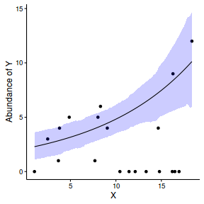
Defining full log-likelihood function
Now lets try it by specifying log-likelihood and the zero trick. When applying this trick, we need to manually calculate the deviance as the inbuilt deviance will be based on the log-likelihood of estimating the zeros (as part of the zero trick) rather than the deviance of the intended model..
The one advantage of the zero trick is that the Deviance and thus DIC, AIC provided by R2jags will be incorrect. Hence, they too need to be manually defined within jags. I suspect that the AIC calculation I have used is incorrect...
Xmat <- model.matrix(~x, dat.zip) nX <- ncol(Xmat) dat.zip.list2 <- with(dat.zip,list(Y=y, X=Xmat,N=nrow(dat.zip), mu=rep(0,nX), Sigma=diag(1.0E-06,nX), zeros=rep(0,nrow(dat)), C=10000)) modelString=" model { for (i in 1:N) { zeros[i] ~ dpois(zeros.lambda[i]) zeros.lambda[i] <- -ll[i] + C ll[i] <- Y[i]*log(lambda[i]) - lambda[i] - loggam(Y[i]+1) eta[i] <- inprod(beta[], X[i,]) log(lambda[i]) <- eta[i] llm[i] <- Y[i]*log(meanlambda) - meanlambda - loggam(Y[i]+1) } meanlambda <- mean(lambda) beta ~ dmnorm(mu[],Sigma[,]) dev <- sum(-2*ll) pD <- mean(dev)-sum(-2*llm) AIC <- min(dev+(2*pD)) } " writeLines(modelString,con='../downloads/BUGSscripts/tut11.5bS1.42.bug') library(R2jags) system.time( dat.ZIP.jags3 <- jags(model=textConnection(modelString), data=dat.zip.list2, inits=NULL, param=c('beta','dev','AIC'), n.chain=3, n.iter=50000, n.thin=50, n.burnin=10000) )
Compiling model graph Resolving undeclared variables Allocating nodes Graph Size: 328 Initializing model
user system elapsed 1.832 0.000 1.839
print(dat.ZIP.jags3)
Inference for Bugs model at "5", fit using jags, 3 chains, each with 50000 iterations (first 10000 discarded), n.thin = 50 n.sims = 2400 iterations saved mu.vect sd.vect 2.5% 25% 50% 75% 97.5% Rhat n.eff AIC 1.215e+02 4.532 117.557 1.185e+02 1.200e+02 1.229e+02 1.336e+02 1.001 2400 beta[1] 6.440e-01 0.336 -0.045 4.270e-01 6.580e-01 8.750e-01 1.252e+00 1.005 480 beta[2] 3.000e-02 0.027 -0.022 1.100e-02 3.000e-02 4.700e-02 8.600e-02 1.005 480 dev 1.220e+02 2.038 120.044 1.206e+02 1.214e+02 1.228e+02 1.274e+02 1.001 2400 deviance 4.001e+05 2.038 400120.044 4.001e+05 4.001e+05 4.001e+05 4.001e+05 1.000 1 For each parameter, n.eff is a crude measure of effective sample size, and Rhat is the potential scale reduction factor (at convergence, Rhat=1). DIC info (using the rule, pD = var(deviance)/2) pD = 2.1 and DIC = 400124.1 DIC is an estimate of expected predictive error (lower deviance is better).Zero-inflated negative binomial (ZINB)
Scenario and Data
Lets say we wanted to model the abundance of an item ($y$) against a continuous predictor ($x$). As this section is mainly about the generation of artificial data (and not specifically about what to do with the data), understanding the actual details are optional and can be safely skipped. Consequently, I have folded (toggled) this section away.
Random data incorporating the following trends (effect parameters)- the sample size = 20
- the continuous $x$ variable is a random uniform spread of measurements between 1 and 20
- the rate of change in log $y$ per unit of $x$ (slope) = 0.1.
- the value of $x$ when log$y$ equals 0 (when $y$=1)
- to generate the values of $y$ expected at each $x$ value, we evaluate the linear predictor (created by calculating the outer product of the model matrix and the regression parameters). These expected values are then transformed into a scale mapped by (0,$\infty$) by using the log function $e^{linear~predictor}$
- finally, we generate $y$ values by using the expected $y$ values ($\lambda$) as probabilities when drawing random numbers from a Poisson distribution. This step adds random noise to the expected $y$ values and returns only 0's and positive integers.
set.seed(37) #34.5 #4 #10 #16 #17 #26 #The number of samples n.x <- 20 #Create x values that at uniformly distributed throughout the rate of 1 to 20 x <- sort(runif(n = n.x, min = 1, max =20)) mm <- model.matrix(~x) intercept <- 0.6 slope=0.1 #The linear predictor linpred <- mm %*% c(intercept,slope) #Predicted y values lambda <- exp(linpred) #Add some noise and make binomial library(gamlss.dist) #fixed latent binomial y<- rZINBI(n.x,lambda, 0.4) #latent binomial influenced by the linear predictor #y<- rZINB(n.x,lambda, 1-exp(linpred)/(1+exp(linpred))) dat.zinb <- data.frame(y,x) summary(dat.glm.nb<-glm.nb(y~x, dat.zinb))
Call: glm.nb(formula = y ~ x, data = dat.zinb, init.theta = 0.4646673144, link = log) Deviance Residuals: Min 1Q Median 3Q Max -1.3578 -1.3455 -0.5069 0.3790 1.1809 Coefficients: Estimate Std. Error z value Pr(>|z|) (Intercept) 0.914191 0.796804 1.147 0.251 x 0.009149 0.067713 0.135 0.893 (Dispersion parameter for Negative Binomial(0.4647) family taken to be 1) Null deviance: 20.303 on 19 degrees of freedom Residual deviance: 20.282 on 18 degrees of freedom AIC: 90.365 Number of Fisher Scoring iterations: 1 Theta: 0.465 Std. Err.: 0.218 2 x log-likelihood: -84.365plot(glm.nb(y~x, dat.zinb))
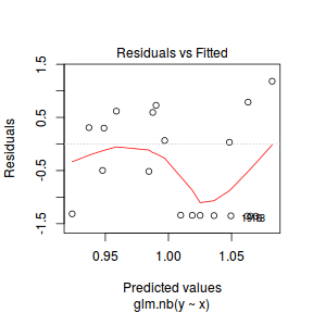
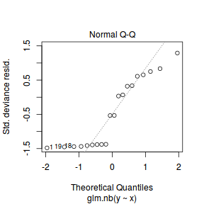
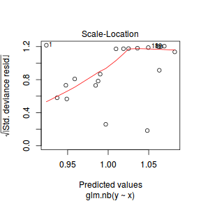
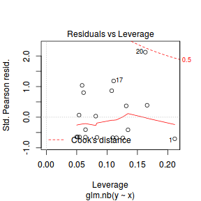
library(pscl) summary(dat.zeroinfl<-zeroinfl(y ~ x | 1, dist = "negbin", data = dat.zinb))
Call: zeroinfl(formula = y ~ x | 1, data = dat.zinb, dist = "negbin") Pearson residuals: Min 1Q Median 3Q Max -0.9609 -0.9268 -0.4446 1.0425 1.7556 Count model coefficients (negbin with log link): Estimate Std. Error z value Pr(>|z|) (Intercept) 0.92733 0.32507 2.853 0.00433 ** x 0.06870 0.02755 2.494 0.01263 * Log(theta) 3.36066 3.59739 0.934 0.35020 Zero-inflation model coefficients (binomial with logit link): Estimate Std. Error z value Pr(>|z|) (Intercept) -0.2250 0.4559 -0.494 0.622 --- Signif. codes: 0 '***' 0.001 '**' 0.01 '*' 0.05 '.' 0.1 ' ' 1 Theta = 28.8082 Number of iterations in BFGS optimization: 17 Log-likelihood: -38.54 on 4 Dfplot(resid(zeroinfl(y ~ x | 1, dist = "negbin", data = dat.zinb))~fitted(zeroinfl(y ~ x | 1, dist = "negbin", data = dat.zinb)))
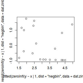
vuong(dat.glm.nb, dat.zeroinfl)
Vuong Non-Nested Hypothesis Test-Statistic: (test-statistic is asymptotically distributed N(0,1) under the null that the models are indistinguishible) ------------------------------------------------------------- Vuong z-statistic H_A p-value Raw -1.2809521 model2 > model1 0.10011 AIC-corrected -0.9296587 model2 > model1 0.17627 BIC-corrected -0.7547616 model2 > model1 0.22520library(gamlss) summary(gamlss(y~x, data=dat.zinb, family='ZINBI'))
GAMLSS-RS iteration 1: Global Deviance = 81.436 GAMLSS-RS iteration 2: Global Deviance = 78.1917 GAMLSS-RS iteration 3: Global Deviance = 77.0798 GAMLSS-RS iteration 4: Global Deviance = 77.0726 GAMLSS-RS iteration 5: Global Deviance = 77.0725 ******************************************************************* Family: c("ZINBI", "Zero inflated negative binomial type I") Call: gamlss(formula = y ~ x, family = "ZINBI", data = dat.zinb) Fitting method: RS() ------------------------------------------------------------------- Mu link function: log Mu Coefficients: Estimate Std. Error t value Pr(>|t|) (Intercept) 0.92653 0.32502 2.851 0.0116 * x 0.06880 0.02753 2.499 0.0237 * --- Signif. codes: 0 '***' 0.001 '**' 0.01 '*' 0.05 '.' 0.1 ' ' 1 ------------------------------------------------------------------- Sigma link function: log Sigma Coefficients: Estimate Std. Error t value Pr(>|t|) (Intercept) -3.363 3.603 -0.933 0.365 ------------------------------------------------------------------- Nu link function: logit Nu Coefficients: Estimate Std. Error t value Pr(>|t|) (Intercept) -0.2250 0.4559 -0.494 0.628 ------------------------------------------------------------------- No. of observations in the fit: 20 Degrees of Freedom for the fit: 4 Residual Deg. of Freedom: 16 at cycle: 5 Global Deviance: 77.0725 AIC: 85.0725 SBC: 89.05543 *******************************************************************summary(gamlss(y~x, nu.fo=y~x,data=dat.zinb, family='ZINBI'))
GAMLSS-RS iteration 1: Global Deviance = 78.2478 GAMLSS-RS iteration 2: Global Deviance = 74.2622 GAMLSS-RS iteration 3: Global Deviance = 73.8329 GAMLSS-RS iteration 4: Global Deviance = 73.8305 GAMLSS-RS iteration 5: Global Deviance = 73.8305 ******************************************************************* Family: c("ZINBI", "Zero inflated negative binomial type I") Call: gamlss(formula = y ~ x, nu.formula = y ~ x, family = "ZINBI", data = dat.zinb) Fitting method: RS() ------------------------------------------------------------------- Mu link function: log Mu Coefficients: Estimate Std. Error t value Pr(>|t|) (Intercept) 0.84246 0.35267 2.389 0.0305 * x 0.07481 0.02933 2.550 0.0222 * --- Signif. codes: 0 '***' 0.001 '**' 0.01 '*' 0.05 '.' 0.1 ' ' 1 ------------------------------------------------------------------- Sigma link function: log Sigma Coefficients: Estimate Std. Error t value Pr(>|t|) (Intercept) -2.982 2.844 -1.048 0.311 ------------------------------------------------------------------- Nu link function: logit Nu Coefficients: Estimate Std. Error t value Pr(>|t|) (Intercept) -2.4988 1.8283 -1.367 0.192 x 0.1996 0.1417 1.408 0.179 ------------------------------------------------------------------- No. of observations in the fit: 20 Degrees of Freedom for the fit: 5 Residual Deg. of Freedom: 15 at cycle: 5 Global Deviance: 73.83046 AIC: 83.83046 SBC: 88.80912 *******************************************************************library(INLA) summary(inla(y~x,data=dat.zinb, family='zeroinflatednbinomial1'))
Call: "inla(formula = y ~ x, family = \"zeroinflatednbinomial1\", data = dat.zinb)" Time used: Pre-processing Running inla Post-processing Total 0.1669 0.0427 0.0285 0.2380 Fixed effects: mean sd 0.025quant 0.5quant 0.975quant mode kld (Intercept) 0.9374 0.7147 -0.4199 0.9152 2.4282 0.8816 0 x 0.0259 0.0625 -0.0982 0.0257 0.1508 0.0254 0 The model has no random effects Model hyperparameters: mean sd 0.025quant 0.5quant 0.975quant mode size for nbinomial zero-inflated observations 0.6180 0.3059 0.1785 0.5699 1.3497 0.4477 zero-probability parameter for zero-inflated nbinomial_1 0.1743 0.1284 0.0142 0.1456 0.4896 0.0431 Expected number of effective parameters(std dev): 2.00(0.00) Number of equivalent replicates : 9.999 Marginal log-Likelihood: -49.48Exploratory data analysis and initial assumption checking
The assumptions are:- All of the observations are independent - this must be addressed at the design and collection stages
- The response variable (and thus the residuals) should be matched by an appropriate distribution (in the case of positive integers response - a Poisson is appropriate).
- All observations are equally influential in determining the trends - or at least no observations are overly influential. This is most effectively diagnosed via residuals and other influence indices and is very difficult to diagnose prior to analysis
- the relationship between the linear predictor (right hand side of the regression formula) and the link function should be linear. A scatterplot with smoother can be useful for identifying possible non-linearity.
- Dispersion is either 1 or overdispersion is otherwise accounted for in the model
- The number of zeros is either not excessive or else they are specifically addressed by the model
Confirm non-normality and explore clumping
Check the distribution of the $y$ abundances
There is definitely signs of non-normality that would warrant Poisson or negative binomial models. Further to that, there appears to be a large number of zeros and a possible clumpiness that are likely to be the cause of overdispersion A zero-inflated negative binomial model is likely to be one of the most effective for modeling these data.hist(dat.zinb$y)
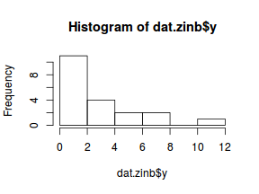
boxplot(dat.zinb$y, horizontal=TRUE) rug(jitter(dat.zinb$y))
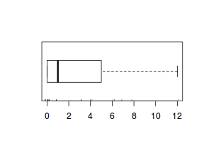
Confirm linearity
Lets now explore linearity by creating a histogram of the predictor variable ($x$). Note, it is difficult to directly assess issues of linearity. Indeed, a scatterplot with lowess smoother will be largely influenced by the presence of zeros. One possible way of doing so is to explore the trend in the non-zero data.
hist(dat.zinb$x)
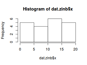
#now for the scatterplot plot(y~x, dat.zinb, log="y") with(subset(dat.zinb,y>0), lines(lowess(y~x)))
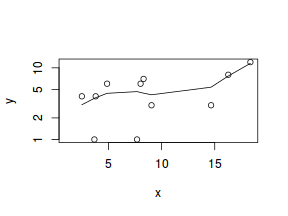
Conclusions: the predictor ($x$) does not display any skewness or other issues that might lead to non-linearity. The lowess smoother on the non-zero data cloud does not display major deviations from a straight line and thus linearity is likely to be satisfied. Violations of linearity (whilst difficult to be certain about due to the unknown influence of the zeros) could be addressed by either:
- define a non-linear linear predictor (such as a polynomial, spline or other non-linear function)
- transform the scale of the predictor variables
Explore zero inflation
Although we have already established that there are few zeros in the data (and thus overdispersion is unlikely to be an issue), we can also explore this by comparing the number of zeros in the data to the number of zeros that would be expected from a Poisson distribution with a mean equal to the mean count of the data.
In the above, the value under FALSE is the proportion of non-zero values in the data and the value under TRUE is the proportion of zeros in the data. In this example, the proportion of zeros observed (#proportion of 0's in the data dat.zinb.tab<-table(dat.zinb$y==0) dat.zinb.tab/sum(dat.zinb.tab)
FALSE TRUE 0.55 0.45
#proportion of 0's expected from a Poisson distribution mu <- mean(dat.zinb$y) v <- var(dat.zinb$y) size <- mu + (mu^2)/v cnts <- rnbinom(1000, mu=mu, size=size) dat.zinb.tabE <- table(cnts == 0) dat.zinb.tabE/sum(dat.zinb.tabE)
FALSE TRUE 0.86 0.14
45%) far exceeds that that would have been expected (14%). Hence it is highly likely that any models will be zero-inflated.Model fitting or statistical analysis
The exploratory data analyses have suggested that a zero-inflated Poisson model might be the most appropriate for these data.
dat.zinb.list <- with(dat.zinb,list(Y=y, X=x,N=nrow(dat.zinb))) modelString=" model { for (i in 1:N) { Y[i] ~ dnegbin(p[i],size) p[i] <- size/(size+mu[i]) eta[i] <- beta0 + beta1*X[i] log(mu[i]) <- eta[i] } size ~ dunif(0.001, 5) beta0 ~ dnorm(0,1.0E-06) beta1 ~ dnorm(0,1.0E-06) } " #writeLines(modelString,con='../downloads/BUGSscripts/tut11.5bS5.4.bug') library(R2jags) system.time( dat.zinb.jags <- jags(model.file=textConnection(modelString), data=dat.zinb.list, inits=NULL, param=c('beta0','beta1', 'size', 'theta'), n.chain=3, n.iter=20000, n.thin=10, n.burnin=10000) )
Compiling model graph Resolving undeclared variables Allocating nodes Graph Size: 148 Initializing model
user system elapsed 11.001 0.004 11.021
print(dat.zinb.jags)
Inference for Bugs model at "5", fit using jags, 3 chains, each with 20000 iterations (first 10000 discarded), n.thin = 10 n.sims = 3000 iterations saved mu.vect sd.vect 2.5% 25% 50% 75% 97.5% Rhat n.eff beta0 1.009 0.826 -0.441 0.450 0.953 1.492 2.859 1.001 2300 beta1 0.010 0.069 -0.125 -0.036 0.010 0.052 0.148 1.001 2000 size 0.545 0.297 0.183 0.348 0.478 0.674 1.237 1.002 1500 deviance 87.531 2.572 84.591 85.630 86.886 88.682 94.252 1.001 3000 For each parameter, n.eff is a crude measure of effective sample size, and Rhat is the potential scale reduction factor (at convergence, Rhat=1). DIC info (using the rule, pD = var(deviance)/2) pD = 3.3 and DIC = 90.8 DIC is an estimate of expected predictive error (lower deviance is better).#extract the samples for the two model parameters coefs <- dat.zinb.jags$BUGSoutput$sims.matrix[,1:2] Xmat <- model.matrix(~x, data=dat) #expected values on a log scale eta<-coefs %*% t(Xmat) #expected value on response scale lambda <- exp(eta) Resid <- -1*sweep(lambda,2,dat.zinb$y, '-')/sqrt(lambda) RSS <- apply(Resid^2, 1, sum) Disp <- RSS/(nrow(dat.zinb)-ncol(coefs)) data.frame(Median=median(Disp), Mean=mean(Disp), HPDinterval(as.mcmc(Disp)), HPDinterval(as.mcmc(Disp),p=0.5))
Median Mean lower upper lower.1 upper.1 var1 5.057138 5.85636 3.303402 10.79281 3.304139 5.058315
JAGS
$$ Y_i = \left\{ \begin{array}{lrcl} 0~\text{with}~P(y_i) = 1-\mu & z_i&\sim&\text{Binom}(1-\theta)\\ & logit(\theta)&=&\gamma_0\\ &\gamma_0&\sim{}&\mathcal{N}(0,10000)\\ >0 & Y_i&\sim&\text{NB}(\lambda_i)\\ &\lambda_i&=&z_i + \eta_i\\ &log(\eta_i)&=&\beta_0+\beta_1x_1\\ &\beta_0, \beta_1&\sim{}&\mathcal{N}(0,10000)\\ \end{array} \right. $$ Or in shorthand: $$ \begin{align} Y_i&\sim{}ZINB(\lambda,\theta) & (\text{response distribution})\\ logit(\theta)&=\gamma_0 & (\text{link function/linear predictor - zero component})\\ log(\lambda_i)&=\eta_i & (\text{link function - count component})\\ \eta_i&=\beta_0+\beta_1 X_i & (\text{linear predictor - count component})\\ \beta_0, \beta_1, \gamma_0&\sim{}\mathcal{N}(0,10000) & (\text{diffuse Bayesian priors})\\ \end{align} $$dat.zinb.list <- with(dat.zinb,list(Y=y, X=x,N=nrow(dat.zinb),z=ifelse(y==0,0,1))) modelString=" model { for (i in 1:N) { z[i] ~ dbern(psi.min) Y[i] ~ dnegbin(p[i],size) p[i] <- size/(size+mu.eff[i]) mu.eff[i] <- z[i]*mu[i] eta[i] <- beta0 + beta1*X[i] log(mu[i]) <- eta[i] } gamma ~ dnorm(0,0.001) psi.min <- min(0.9999, max(0.00001, (1-psi))) logit(psi) <- max(-20, min(20, gamma)) size ~ dunif(0.001, 5) theta <- pow(1/mean(p),2) beta0 ~ dnorm(0,1.0E-06) beta1 ~ dnorm(0,1.0E-06) } " system.time( dat.zinb.jags <- jags(model.file=textConnection(modelString), data=dat.zinb.list, inits=NULL, param=c('beta0','beta1', 'size', 'theta'), n.chain=3, n.iter=20000, n.thin=10, n.burnin=10000) )
Compiling model graph Resolving undeclared variables Allocating nodes Graph Size: 205 Initializing model
user system elapsed 12.241 0.000 12.273
print(dat.zinb.jags)
Inference for Bugs model at "5", fit using jags, 3 chains, each with 20000 iterations (first 10000 discarded), n.thin = 10 n.sims = 3000 iterations saved mu.vect sd.vect 2.5% 25% 50% 75% 97.5% Rhat n.eff beta0 0.961 0.449 0.077 0.661 0.962 1.258 1.851 1.001 2300 beta1 0.067 0.041 -0.009 0.039 0.066 0.095 0.152 1.001 3000 size 3.503 1.010 1.402 2.781 3.647 4.348 4.930 1.001 3000 theta 2.196 0.367 1.718 1.938 2.109 2.363 3.145 1.001 3000 deviance 82.682 2.814 79.127 80.610 82.086 84.011 89.900 1.001 3000 For each parameter, n.eff is a crude measure of effective sample size, and Rhat is the potential scale reduction factor (at convergence, Rhat=1). DIC info (using the rule, pD = var(deviance)/2) pD = 4.0 and DIC = 86.6 DIC is an estimate of expected predictive error (lower deviance is better).Xmat <- model.matrix(~x, dat.zip) nX <- ncol(Xmat) dat.zip.list1 <- with(dat.zip,list(Y=y, X=Xmat,N=nrow(dat.zip), nX=nX, z=ifelse(y==0,0,1))) modelString=" model { for (i in 1:N) { z[i] ~ dbern(psi.min) Y[i] ~ dnegbin(p[i],size) p[i] <- size/(size+mu.eff[i]) mu.eff[i] <- z[i]*mu[i] log(mu[i]) <- inprod(beta[], X[i,]) } gamma ~ dnorm(0,0.001) psi.min <- min(0.9999, max(0.00001, (1-psi))) logit(psi) <- max(-20, min(20, gamma)) size ~ dunif(0.001, 5) theta <- pow(1/mean(p),2) for (i in 1:nX) { beta[i] ~ dnorm(0,1.0E-06) } } " library(R2jags) system.time( dat.zip.jags1 <- jags(model.file=textConnection(modelString), data=dat.zip.list1, inits=NULL, param=c('beta','gamma0'), n.chain=3, n.iter=20000, n.thin=10, n.burnin=10000) )
Compiling model graph Resolving undeclared variables Allocating nodes Graph Size: 227 Initializing model
user system elapsed 12.389 0.004 12.411
print(dat.zip.jags1)
Inference for Bugs model at "5", fit using jags, 3 chains, each with 20000 iterations (first 10000 discarded), n.thin = 10 n.sims = 3000 iterations saved mu.vect sd.vect 2.5% 25% 50% 75% 97.5% Rhat n.eff beta[1] 0.753 0.453 -0.143 0.448 0.743 1.069 1.633 1.001 3000 beta[2] 0.084 0.041 0.006 0.056 0.084 0.111 0.167 1.001 3000 deviance 80.373 2.924 76.666 78.234 79.724 81.807 87.799 1.001 3000 For each parameter, n.eff is a crude measure of effective sample size, and Rhat is the potential scale reduction factor (at convergence, Rhat=1). DIC info (using the rule, pD = var(deviance)/2) pD = 4.3 and DIC = 84.7 DIC is an estimate of expected predictive error (lower deviance is better).Or arguably better still, use a multivariate normal prior. If we have a $k$ regression parameters ($\beta_k$), then the multivariate normal priors are defined as: $$ \boldsymbol{\beta}\sim{}\mathcal{N_k}(\boldsymbol{\mu}, \mathbf{\Sigma}) $$ where $$\boldsymbol{\mu}=[E[\beta_1],E[\beta_2],...,E[\beta_k]] = \left(\begin{array}{c}0\\\vdots\\0\end{array}\right)$$ $$ \mathbf{\Sigma}=[Cov[\beta_i, \beta_j]] = \left(\begin{array}{ccc}1000^2&0&0\\0&\ddots&0\\0&0&1000^2\end{array} \right) $$ hence, along with the response and predictor matrix, we need to supply $\boldsymbol{\mu}$ (a vector of zeros) and $\boldsymbol{\Sigma}$ (a covariance matrix with $1000^2$ in the diagonals).
Xmat <- model.matrix(~x, dat.zip) nX <- ncol(Xmat) dat.zip.list2 <- with(dat.zip,list(Y=y, X=Xmat,N=nrow(dat.zip), nX=nX, mu=rep(0,nX),Sigma=diag(1.0E-06,nX), z=ifelse(y==0,0,1))) modelString=" model { for (i in 1:N) { z[i] ~ dbern(psi.min) Y[i] ~ dnegbin(p[i],size) p[i] <- size/(size+mu.eff[i]) mu.eff[i] <- z[i]*eta[i] log(eta[i]) <- inprod(beta[], X[i,]) } gamma ~ dnorm(0,0.001) psi.min <- min(0.9999, max(0.00001, (1-psi))) logit(psi) <- max(-20, min(20, gamma)) size ~ dunif(0.001, 5) theta <- pow(1/mean(p),2) beta ~ dmnorm(mu[],Sigma[,]) } " library(R2jags) system.time( dat.zip.jags2 <- jags(model.file=textConnection(modelString), data=dat.zip.list2, inits=NULL, param=c('beta','gamma','size','theta'), n.chain=3, n.iter=20000, n.thin=10, n.burnin=10000) )
Compiling model graph Resolving undeclared variables Allocating nodes Graph Size: 231 Initializing model
user system elapsed 5.220 0.004 5.234
print(dat.zip.jags2)
Inference for Bugs model at "5", fit using jags, 3 chains, each with 20000 iterations (first 10000 discarded), n.thin = 10 n.sims = 3000 iterations saved mu.vect sd.vect 2.5% 25% 50% 75% 97.5% Rhat n.eff beta[1] 0.757 0.453 -0.155 0.453 0.772 1.063 1.620 1.001 3000 beta[2] 0.084 0.041 0.007 0.056 0.084 0.112 0.168 1.001 3000 gamma -0.201 0.455 -1.131 -0.505 -0.186 0.104 0.655 1.003 940 size 3.661 0.954 1.563 3.006 3.830 4.462 4.946 1.002 1300 theta 2.104 0.320 1.673 1.884 2.039 2.249 2.938 1.003 850 deviance 80.435 2.902 76.659 78.327 79.800 81.843 87.741 1.002 1300 For each parameter, n.eff is a crude measure of effective sample size, and Rhat is the potential scale reduction factor (at convergence, Rhat=1). DIC info (using the rule, pD = var(deviance)/2) pD = 4.2 and DIC = 84.6 DIC is an estimate of expected predictive error (lower deviance is better).dat.zinb.brm <- brm(y~0+spec + main + main:x, data=dat.zinb, family='zero_inflated_negbinomial', prior = c(set_prior("normal(0,10)", class="b", coef="main"), set_prior("normal(0,100)", class="b", coef="spec"), set_prior("student_t(3,0,5)", class='shape')), chains=3, iter=5000, warmup=2500, thin=2)
SAMPLING FOR MODEL 'zero_inflated_negbinomial(log) brms-model' NOW (CHAIN 1). Chain 1, Iteration: 1 / 5000 [ 0%] (Warmup) Chain 1, Iteration: 500 / 5000 [ 10%] (Warmup) Chain 1, Iteration: 1000 / 5000 [ 20%] (Warmup) Chain 1, Iteration: 1500 / 5000 [ 30%] (Warmup) Chain 1, Iteration: 2000 / 5000 [ 40%] (Warmup) Chain 1, Iteration: 2500 / 5000 [ 50%] (Warmup) Chain 1, Iteration: 2501 / 5000 [ 50%] (Sampling) Chain 1, Iteration: 3000 / 5000 [ 60%] (Sampling) Chain 1, Iteration: 3500 / 5000 [ 70%] (Sampling) Chain 1, Iteration: 4000 / 5000 [ 80%] (Sampling) Chain 1, Iteration: 4500 / 5000 [ 90%] (Sampling) Chain 1, Iteration: 5000 / 5000 [100%] (Sampling)# # Elapsed Time: 1.52902 seconds (Warm-up) # 0.555669 seconds (Sampling) # 2.08469 seconds (Total) # SAMPLING FOR MODEL 'zero_inflated_negbinomial(log) brms-model' NOW (CHAIN 2). Chain 2, Iteration: 1 / 5000 [ 0%] (Warmup) Chain 2, Iteration: 500 / 5000 [ 10%] (Warmup) Chain 2, Iteration: 1000 / 5000 [ 20%] (Warmup) Chain 2, Iteration: 1500 / 5000 [ 30%] (Warmup) Chain 2, Iteration: 2000 / 5000 [ 40%] (Warmup) Chain 2, Iteration: 2500 / 5000 [ 50%] (Warmup) Chain 2, Iteration: 2501 / 5000 [ 50%] (Sampling) Chain 2, Iteration: 3000 / 5000 [ 60%] (Sampling) Chain 2, Iteration: 3500 / 5000 [ 70%] (Sampling) Chain 2, Iteration: 4000 / 5000 [ 80%] (Sampling) Chain 2, Iteration: 4500 / 5000 [ 90%] (Sampling) Chain 2, Iteration: 5000 / 5000 [100%] (Sampling)# # Elapsed Time: 1.33141 seconds (Warm-up) # 0.635069 seconds (Sampling) # 1.96648 seconds (Total) # SAMPLING FOR MODEL 'zero_inflated_negbinomial(log) brms-model' NOW (CHAIN 3). Chain 3, Iteration: 1 / 5000 [ 0%] (Warmup) Chain 3, Iteration: 500 / 5000 [ 10%] (Warmup) Chain 3, Iteration: 1000 / 5000 [ 20%] (Warmup) Chain 3, Iteration: 1500 / 5000 [ 30%] (Warmup) Chain 3, Iteration: 2000 / 5000 [ 40%] (Warmup) Chain 3, Iteration: 2500 / 5000 [ 50%] (Warmup) Chain 3, Iteration: 2501 / 5000 [ 50%] (Sampling) Chain 3, Iteration: 3000 / 5000 [ 60%] (Sampling) Chain 3, Iteration: 3500 / 5000 [ 70%] (Sampling) Chain 3, Iteration: 4000 / 5000 [ 80%] (Sampling) Chain 3, Iteration: 4500 / 5000 [ 90%] (Sampling) Chain 3, Iteration: 5000 / 5000 [100%] (Sampling)# # Elapsed Time: 1.19223 seconds (Warm-up) # 2.45475 seconds (Sampling) # 3.64698 seconds (Total) #
## Or if we allow the zero-inflation model and the count model to vary with x dat.zinb.brm1 <- brm(y~trait:x, data=dat.zinb, family='zero_inflated_negbinomial', prior = c(set_prior("normal(0,100)", class="Intercept"), set_prior("normal(0,10)", class="b", coef="traity:x"), set_prior("normal(0,10)", class="b", coef="traitzi_y:x"), set_prior("student_t(3,0,5)", class='shape')), chains=3, iter=5000, warmup=2500, thin=2)
SAMPLING FOR MODEL 'zero_inflated_negbinomial(log) brms-model' NOW (CHAIN 1). Chain 1, Iteration: 1 / 5000 [ 0%] (Warmup) Chain 1, Iteration: 500 / 5000 [ 10%] (Warmup) Chain 1, Iteration: 1000 / 5000 [ 20%] (Warmup) Chain 1, Iteration: 1500 / 5000 [ 30%] (Warmup) Chain 1, Iteration: 2000 / 5000 [ 40%] (Warmup) Chain 1, Iteration: 2500 / 5000 [ 50%] (Warmup) Chain 1, Iteration: 2501 / 5000 [ 50%] (Sampling) Chain 1, Iteration: 3000 / 5000 [ 60%] (Sampling) Chain 1, Iteration: 3500 / 5000 [ 70%] (Sampling) Chain 1, Iteration: 4000 / 5000 [ 80%] (Sampling) Chain 1, Iteration: 4500 / 5000 [ 90%] (Sampling) Chain 1, Iteration: 5000 / 5000 [100%] (Sampling)# # Elapsed Time: 8.43611 seconds (Warm-up) # 12.464 seconds (Sampling) # 20.9001 seconds (Total) # SAMPLING FOR MODEL 'zero_inflated_negbinomial(log) brms-model' NOW (CHAIN 2). Chain 2, Iteration: 1 / 5000 [ 0%] (Warmup) Chain 2, Iteration: 500 / 5000 [ 10%] (Warmup) Chain 2, Iteration: 1000 / 5000 [ 20%] (Warmup) Chain 2, Iteration: 1500 / 5000 [ 30%] (Warmup) Chain 2, Iteration: 2000 / 5000 [ 40%] (Warmup) Chain 2, Iteration: 2500 / 5000 [ 50%] (Warmup) Chain 2, Iteration: 2501 / 5000 [ 50%] (Sampling) Chain 2, Iteration: 3000 / 5000 [ 60%] (Sampling) Chain 2, Iteration: 3500 / 5000 [ 70%] (Sampling) Chain 2, Iteration: 4000 / 5000 [ 80%] (Sampling) Chain 2, Iteration: 4500 / 5000 [ 90%] (Sampling) Chain 2, Iteration: 5000 / 5000 [100%] (Sampling)# # Elapsed Time: 5.60244 seconds (Warm-up) # 8.82955 seconds (Sampling) # 14.432 seconds (Total) # SAMPLING FOR MODEL 'zero_inflated_negbinomial(log) brms-model' NOW (CHAIN 3). Chain 3, Iteration: 1 / 5000 [ 0%] (Warmup) Chain 3, Iteration: 500 / 5000 [ 10%] (Warmup) Chain 3, Iteration: 1000 / 5000 [ 20%] (Warmup) Chain 3, Iteration: 1500 / 5000 [ 30%] (Warmup) Chain 3, Iteration: 2000 / 5000 [ 40%] (Warmup) Chain 3, Iteration: 2500 / 5000 [ 50%] (Warmup) Chain 3, Iteration: 2501 / 5000 [ 50%] (Sampling) Chain 3, Iteration: 3000 / 5000 [ 60%] (Sampling) Chain 3, Iteration: 3500 / 5000 [ 70%] (Sampling) Chain 3, Iteration: 4000 / 5000 [ 80%] (Sampling) Chain 3, Iteration: 4500 / 5000 [ 90%] (Sampling) Chain 3, Iteration: 5000 / 5000 [100%] (Sampling)# # Elapsed Time: 8.60118 seconds (Warm-up) # 18.1576 seconds (Sampling) # 26.7588 seconds (Total) #
Chain mixing and Model validation
Prior to exploring the model parameters, it is prudent to confirm that the model did indeed fit the assumptions and was an appropriate fit to the data as well as that the MCMC sampling chain was adequately mixed and the retained samples independent.
- We will start by exploring the mixing of the MCMC chains via traceplots.
plot(as.mcmc(dat.zinb.jags))
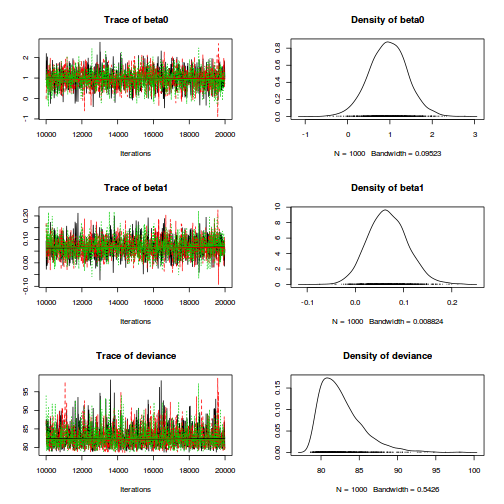
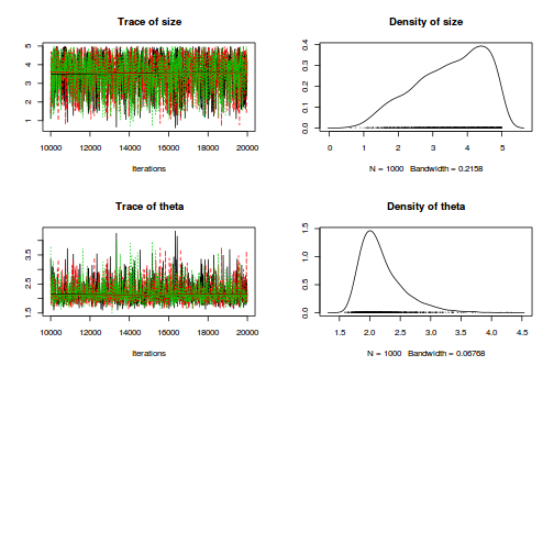
library(gridExtra) grid.arrange(stan_trace(dat.zinb.brm$fit, ncol=1), stan_dens(dat.zinb.brm$fit, separate_chains=TRUE,ncol=1), ncol=2)
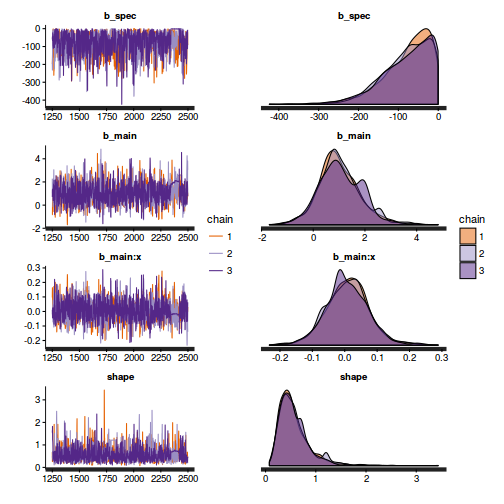
The chains appear well mixed and stable
- Next we will explore correlation amongst MCMC samples.
autocorr.diag(as.mcmc(dat.zinb.jags))
beta0 beta1 deviance size theta Lag 0 1.000000000 1.000000000 1.000000000 1.000000000 1.00000000 Lag 10 0.157707113 0.164120975 0.046293478 0.005759824 -0.01817507 Lag 50 -0.000258746 0.023917373 -0.002086921 0.005145297 -0.01124115 Lag 100 0.001276269 0.002424773 -0.017995644 -0.035551481 -0.03951204 Lag 500 -0.007191282 0.005616019 -0.021469518 -0.044121841 -0.05450130
The level of auto-correlation at the nominated lag of 10 is higher than we would generally like. It is worth increasing the thinning rate from 10 to 50. Obviously, to support this higher thinning rate, we would also increase the number of iterations.
library(R2jags) modelString=" model { for (i in 1:N) { z[i] ~ dbern(psi.min) Y[i] ~ dnegbin(p[i],size) p[i] <- size/(size+mu.eff[i]) mu.eff[i] <- z[i]*mu[i] eta[i] <- beta0 + beta1*X[i] log(mu[i]) <- eta[i] } gamma ~ dnorm(0,0.001) psi.min <- min(0.9999, max(0.00001, (1-psi))) logit(psi) <- max(-20, min(20, gamma)) size ~ dunif(0.001, 5) theta <- pow(1/mean(p),2) beta0 ~ dnorm(0,1.0E-06) beta1 ~ dnorm(0,1.0E-06) } " dat.zinb.jags <- jags(data=dat.zinb.list,model.file=textConnection(modelString), param=c('beta0','beta1','gamma','theta','psi'), n.chains=3, n.iter=100000, n.burnin=50000, n.thin=50)
Compiling model graph Resolving undeclared variables Allocating nodes Graph Size: 205 Initializing model
print(dat.zinb.jags)
Inference for Bugs model at "5", fit using jags, 3 chains, each with 1e+05 iterations (first 50000 discarded), n.thin = 50 n.sims = 3000 iterations saved mu.vect sd.vect 2.5% 25% 50% 75% 97.5% Rhat n.eff beta0 0.973 0.453 0.058 0.679 0.961 1.269 1.882 1.001 3000 beta1 0.066 0.042 -0.014 0.037 0.065 0.094 0.151 1.001 3000 gamma -0.210 0.462 -1.133 -0.521 -0.202 0.090 0.674 1.002 1200 psi 0.450 0.109 0.244 0.373 0.450 0.522 0.662 1.003 1000 theta 2.190 0.363 1.724 1.939 2.102 2.360 3.133 1.001 3000 deviance 82.759 2.824 79.157 80.658 82.132 84.199 89.605 1.001 3000 For each parameter, n.eff is a crude measure of effective sample size, and Rhat is the potential scale reduction factor (at convergence, Rhat=1). DIC info (using the rule, pD = var(deviance)/2) pD = 4.0 and DIC = 86.7 DIC is an estimate of expected predictive error (lower deviance is better).plot(as.mcmc(dat.zinb.jags))
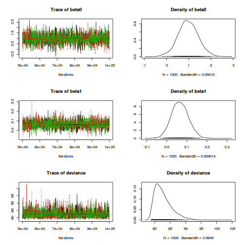
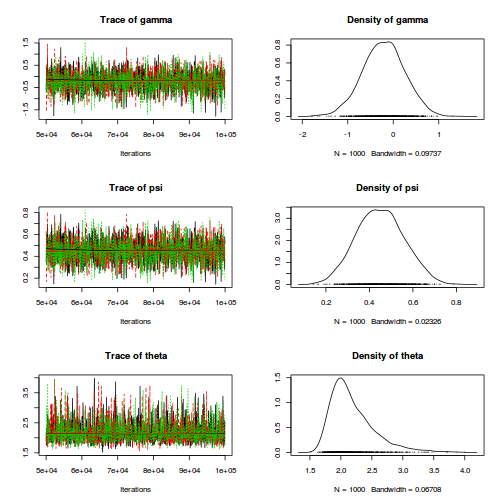
autocorr.diag(as.mcmc(dat.zinb.jags))
beta0 beta1 deviance gamma psi theta Lag 0 1.000000000 1.0000000000 1.000000000 1.000000000 1.000000000 1.0000000000 Lag 50 0.008803828 0.0071072063 0.009745184 0.041114460 0.041195791 -0.0009151277 Lag 250 0.003371794 0.0007720164 -0.006544352 0.012836461 0.014694728 0.0298401324 Lag 500 -0.027820267 -0.0299358791 0.004795827 -0.005996009 -0.007053143 0.0094320909 Lag 2500 0.015181957 0.0200111646 -0.024418362 -0.019640184 -0.020398216 -0.0171605926
stan_ac(dat.zinb.brm$fit)
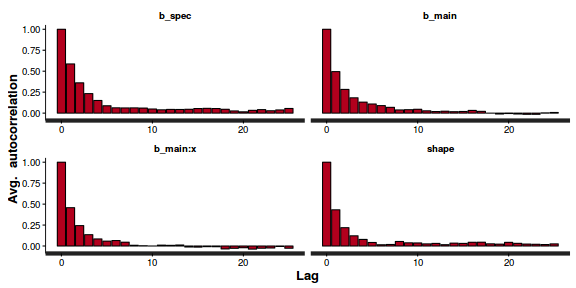
#these samples are highly correlated, lets thin more... dat.zinb.brm <- brm(y~0+spec + main + main:x, data=dat.zinb, family='zero_inflated_negbinomial', prior = c(set_prior("normal(0,10)", class="b", coef="main"), set_prior("normal(0,100)", class="b", coef="spec"), set_prior("student_t(3,0,5)", class='shape')), chains=3, iter=5000, warmup=2500, thin=5)
SAMPLING FOR MODEL 'zero_inflated_negbinomial(log) brms-model' NOW (CHAIN 1). Chain 1, Iteration: 1 / 5000 [ 0%] (Warmup) Chain 1, Iteration: 500 / 5000 [ 10%] (Warmup) Chain 1, Iteration: 1000 / 5000 [ 20%] (Warmup) Chain 1, Iteration: 1500 / 5000 [ 30%] (Warmup) Chain 1, Iteration: 2000 / 5000 [ 40%] (Warmup) Chain 1, Iteration: 2500 / 5000 [ 50%] (Warmup) Chain 1, Iteration: 2501 / 5000 [ 50%] (Sampling) Chain 1, Iteration: 3000 / 5000 [ 60%] (Sampling) Chain 1, Iteration: 3500 / 5000 [ 70%] (Sampling) Chain 1, Iteration: 4000 / 5000 [ 80%] (Sampling) Chain 1, Iteration: 4500 / 5000 [ 90%] (Sampling) Chain 1, Iteration: 5000 / 5000 [100%] (Sampling)# # Elapsed Time: 1.51449 seconds (Warm-up) # 0.541013 seconds (Sampling) # 2.05551 seconds (Total) # SAMPLING FOR MODEL 'zero_inflated_negbinomial(log) brms-model' NOW (CHAIN 2). Chain 2, Iteration: 1 / 5000 [ 0%] (Warmup) Chain 2, Iteration: 500 / 5000 [ 10%] (Warmup) Chain 2, Iteration: 1000 / 5000 [ 20%] (Warmup) Chain 2, Iteration: 1500 / 5000 [ 30%] (Warmup) Chain 2, Iteration: 2000 / 5000 [ 40%] (Warmup) Chain 2, Iteration: 2500 / 5000 [ 50%] (Warmup) Chain 2, Iteration: 2501 / 5000 [ 50%] (Sampling) Chain 2, Iteration: 3000 / 5000 [ 60%] (Sampling) Chain 2, Iteration: 3500 / 5000 [ 70%] (Sampling) Chain 2, Iteration: 4000 / 5000 [ 80%] (Sampling) Chain 2, Iteration: 4500 / 5000 [ 90%] (Sampling) Chain 2, Iteration: 5000 / 5000 [100%] (Sampling)# # Elapsed Time: 1.15206 seconds (Warm-up) # 0.525064 seconds (Sampling) # 1.67712 seconds (Total) # SAMPLING FOR MODEL 'zero_inflated_negbinomial(log) brms-model' NOW (CHAIN 3). Chain 3, Iteration: 1 / 5000 [ 0%] (Warmup) Chain 3, Iteration: 500 / 5000 [ 10%] (Warmup) Chain 3, Iteration: 1000 / 5000 [ 20%] (Warmup) Chain 3, Iteration: 1500 / 5000 [ 30%] (Warmup) Chain 3, Iteration: 2000 / 5000 [ 40%] (Warmup) Chain 3, Iteration: 2500 / 5000 [ 50%] (Warmup) Chain 3, Iteration: 2501 / 5000 [ 50%] (Sampling) Chain 3, Iteration: 3000 / 5000 [ 60%] (Sampling) Chain 3, Iteration: 3500 / 5000 [ 70%] (Sampling) Chain 3, Iteration: 4000 / 5000 [ 80%] (Sampling) Chain 3, Iteration: 4500 / 5000 [ 90%] (Sampling) Chain 3, Iteration: 5000 / 5000 [100%] (Sampling)# # Elapsed Time: 1.09119 seconds (Warm-up) # 2.19041 seconds (Sampling) # 3.2816 seconds (Total) #
stan_ac(dat.zinb.brm$fit)
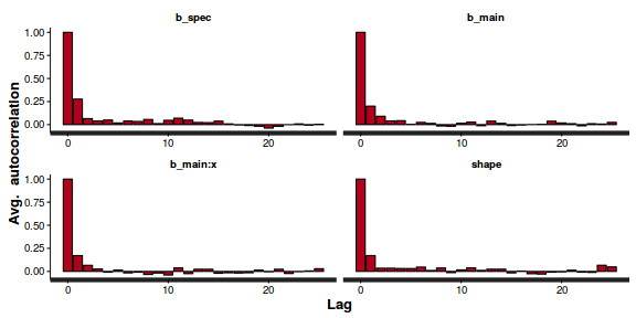
Conclusions: the samples are now less auto-correlated and the chains are all well mixed and appear stable.
- Explore the step size characteristics (STAN only)
Conclusions: acceptance ratio is very good, the lot posterior is relatively robust to step size and tree depth, rhat values are all below 1.05, the effective sample size is not too bad (we might be able to achieve better acceptance ratios with tighter priors) and the ratio of MCMC error to posterior sd is very small.
summary(do.call(rbind, args = get_sampler_params(dat.zip.brm$fit, inc_warmup = FALSE)), digits = 2)
accept_stat__ stepsize__ treedepth__ n_leapfrog__ n_divergent__ Min. :0.19 Min. :0.29 Min. :1.0 Min. : 1.0 Min. :0 1st Qu.:0.89 1st Qu.:0.29 1st Qu.:2.0 1st Qu.: 3.0 1st Qu.:0 Median :0.96 Median :0.35 Median :3.0 Median : 7.0 Median :0 Mean :0.92 Mean :0.33 Mean :2.9 Mean : 7.6 Mean :0 3rd Qu.:0.99 3rd Qu.:0.36 3rd Qu.:4.0 3rd Qu.:11.0 3rd Qu.:0 Max. :1.00 Max. :0.36 Max. :4.0 Max. :15.0 Max. :0
stan_diag(dat.zinb.brm$fit)
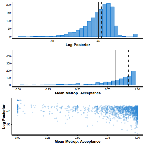
stan_diag(dat.zinb.brm$fit, information = "stepsize")
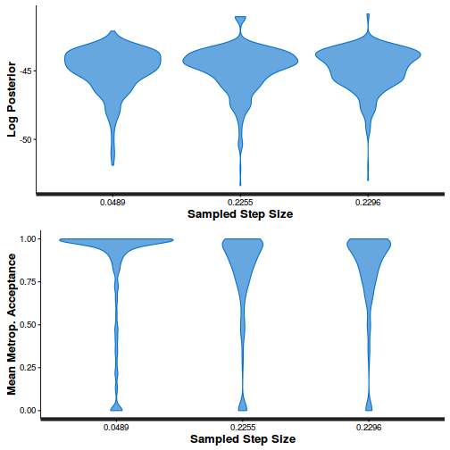
stan_diag(dat.zinb.brm$fit, information = "treedepth")
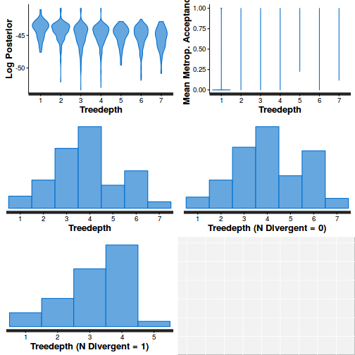
stan_diag(dat.zinb.brm$fit, information = "divergence")
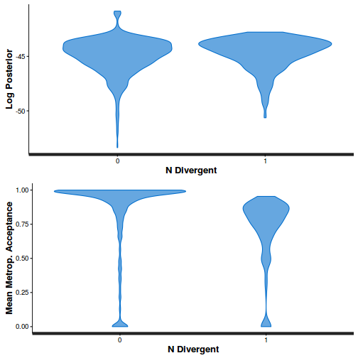
library(gridExtra) grid.arrange(stan_rhat(dat.zinb.brm$fit) + theme_classic(8), stan_ess(dat.zinb.brm$fit) + theme_classic(8), stan_mcse(dat.zinb.brm$fit) + theme_classic(8), ncol = 2)
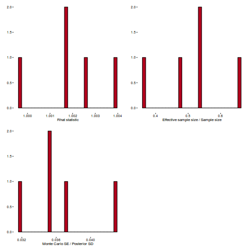
- We now explore the goodness of fit of the models via the residuals and deviance.
We could calculate the Pearsons's residuals within the JAGS model.
Alternatively, we could use the parameters to generate the residuals outside of JAGS.
#extract the samples for the two model parameters coefs <- dat.zinb.jags$BUGSoutput$sims.matrix[,1:2] theta <- dat.zinb.jags$BUGSoutput$sims.matrix[,'psi'] Xmat <- model.matrix(~x, data=dat.zinb) #expected values on a log scale lambda<-coefs %*% t(Xmat) #expected value on response scale eta <- exp(lambda) expY <- sweep(eta,1,(1-theta),"*") varY <- eta+sweep(eta^2,1,theta,"*") head(varY)
1 2 3 4 5 6 7 8 9 10 11 12 13 14 15 16 17 18 19 20 [1,] 5.343355 6.056455 6.710940 6.782673 7.454279 9.591883 9.886422 10.142129 10.857296 12.334728 13.53727 14.42609 16.15161 18.32106 18.55017 21.24417 21.39110 21.82541 22.82726 26.16783 [2,] 6.136290 8.213971 10.463062 10.730368 13.440247 24.739116 26.636896 28.354937 33.515421 45.900953 57.78469 67.65739 89.58710 122.59671 126.45037 177.25918 180.32847 189.58587 212.00514 297.82859 [3,] 11.086488 11.972272 12.745761 12.828478 13.585024 15.812014 16.100779 16.348390 17.026571 18.367469 19.40679 20.14872 21.53308 23.18303 23.35205 25.27383 25.37541 25.67387 26.35240 28.52397 [4,] 5.390940 5.903767 6.358283 6.407248 6.858209 8.216792 8.396190 8.550587 8.976105 9.828478 10.49885 10.98238 11.89530 13.00082 13.11511 14.42760 14.49762 14.70375 15.17440 16.69918 [5,] 5.011368 6.014766 6.990161 7.100137 8.158381 11.852450 12.398287 12.879089 14.257358 17.255958 19.84063 21.83053 25.87864 31.29833 31.89134 39.14718 39.55753 40.77912 43.64564 53.67698 [6,] 20.534217 22.189351 23.632622 23.786853 25.196463 29.335264 29.870784 30.329775 31.585938 34.065499 35.98370 37.35109 39.89831 42.92726 43.23714 46.75510 46.94078 47.48620 48.72534 52.68347
varY <- sweep(varY,1,(1-theta),'*') #sweep across rows and then divide by lambda Resid <- -1*sweep(expY,2,dat.zinb$y,'-')/sqrt(varY) #plot residuals vs expected values plot(apply(Resid,2,mean)~apply(eta,2,mean))
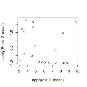
#Calculate residuals coefs.zinb <- as.matrix(as.data.frame(rstan:::extract(dat.zinb.brm$fit))) coefs.zinb <- coefs.zinb[,grep('b_main', colnames(coefs.zinb))] shape <- as.matrix(as.data.frame(rstan:::extract(dat.zinb.brm$fit,'shape'))) Xmat <- model.matrix(~x, data=dat.zinb) lambda.zinb<-coefs.zinb %*% t(Xmat) #expected value on response scale eta.zinb <- exp(lambda.zinb) expY.zinb <- sweep(eta.zinb,1,(1-shape),"*") varY.zinb <- eta.zinb+sweep(eta.zinb^2,1,shape,"*") varY.zinb <- sweep(varY.zinb,1,(1-theta),'*') #sweep across rows and then divide by lambda Resid.zinb <- -1*sweep(expY.zinb,2,dat.zinb$y,'-')/sqrt(varY.zinb) ggplot(data=NULL, aes(y=apply(Resid.zinb,2,mean), x=apply(eta.zinb,2,mean))) + geom_point()
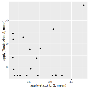
There are no real patterns in the residuals.
- Now we will compare the sum of squared residuals to the sum of squares residuals that would be expected from a Poisson distribution
matching that estimated by the model. Essentially this is estimating how well the Poisson distribution, the log-link function and the linear model
approximates the observed data.
When doing so, we need to consider the expected value and variance of the zero-inflated poisson. $$ E(y_i) = \lambda\times(1-\theta)\\ Var(y_i) = \lambda\times(1-\theta)\times(1+\theta\times\lambda^2) $$
SSres<-apply(Resid^2,1,sum) set.seed(2) #generate a matrix of draws from a zero-inflated poisson (ZINB) distribution # the matrix is the same dimensions as lambda library(gamlss.dist) #YNew <- matrix(rZINB(length(lambda),eta, theta),nrow=nrow(lambda)) lambda <- sweep(eta,1,ifelse(dat.zinb$y==0,0,1),'*') YNew <- matrix(rpois(length(lambda),lambda),nrow=nrow(lambda)) Resid1<-(expY - YNew)/sqrt(varY) SSres.sim<-apply(Resid1^2,1,sum) mean(SSres.sim>SSres)
[1] 0.349
Whilst not ideal (as we would prefer a Bayesian P-value of around 0.5), this value is not wildly bad and does not constitute overwhelming evidence of a lack of fit.
Xmat <- model.matrix(~x, dat.zinb) nX <- ncol(Xmat) dat.zinb.list2 <- with(dat.zinb,list(Y=y, X=Xmat,N=nrow(dat.zinb), nX=nX, mu=rep(0,nX),Sigma=diag(1.0E-06,nX), z=ifelse(y==0,0,1))) modelString=" model { for (i in 1:N) { z[i] ~ dbern(psi.min) Y[i] ~ dnegbin(p[i],size) p[i] <- size/(size+mu.eff[i]) mu.eff[i] <- z[i]*eta[i] log(eta[i]) <- beta0 + beta1*X[i] expY[i] <- eta[i]*(1-psi) varY[i] <- (1-psi)*(eta[i]*psi*pow(eta[i],2)) Resid[i] <- (Y[i] - expY[i])/sqrt(varY[i]) Y1[i] ~ dnegbin(p[i], size) Resid1[i] <- (Y1[i] - expY[i])/sqrt(varY[i]) RSS[i] <- pow(Resid[i],2) RSS1[i] <-pow(Resid1[i],2) } gamma ~ dnorm(0,0.001) psi.min <- min(0.9999, max(0.00001, (1-psi))) logit(psi) <- max(-20, min(20, gamma)) size ~ dunif(0.001, 5) theta <- pow(1/mean(p),2) beta ~ dmnorm(mu[],Sigma[,]) Pvalue <- mean(sum(RSS1)>sum(RSS)) } " writeLines(modelString,con='../downloads/BUGSscripts/tut11.5bS5.13.bug') library(R2jags) system.time( dat.zinb.jags3 <- jags(model='../downloads/BUGSscripts/tut11.5bS5.13.bug', data=dat.zinb.list2, inits=NULL, param=c('beta', 'gamma0','Pvalue'), n.chain=3, n.iter=20000, n.thin=10, n.burnin=10000) )
Compiling model graph Resolving undeclared variables Allocating nodes Deleting model
Error in jags.model(model.file, data = data, inits = init.values, n.chains = n.chains, : RUNTIME ERROR: Compilation error on line 5. Unable to resolve node p[1] This may be due to an undefined ancestor node or a directed cycle in the graph
Timing stopped at: 0.012 0 0.009
print(dat.zinb.jags3)
Error in print(dat.zinb.jags3): error in evaluating the argument 'x' in selecting a method for function 'print': Error: object 'dat.zinb.jags3' not found
SSres.zinb<-apply(Resid.zinb^2,1,sum) set.seed(2) #generate a matrix of draws from a zero-inflated poisson (ZINB) distribution # the matrix is the same dimensions as lambda library(gamlss.dist) #YNew <- matrix(rZINB(length(lambda),eta, theta),nrow=nrow(lambda)) lambda.zinb <- sweep(eta.zinb,1,ifelse(dat.zinb$y==0,0,1),'*') YNew.zinb <- matrix(MASS:::rnegbin(length(lambda.zinb),lambda.zinb, theta=mean(shape)), nrow=nrow(lambda.zinb)) Resid1.zinb<-(expY.zinb - YNew.zinb)/sqrt(varY.zinb) SSres.sim<-apply(Resid1.zinb^2,1,sum) mean(SSres.sim>SSres.zinb)
[1] 0.3206667
Conclusions: the Bayesian p-value is very close to 0.5, suggesting that there is a good fit of the model to the data.
- Since it is difficult to diagnose many issues from the typical residuals we will now explore simulated residuals.
The trend (black symbols) in the qq-plot does not appear to be overly non-linear (matching the ideal red line well), suggesting that the model is not overdispersed. The spread of standardized (simulated) residuals in the residual plot do not appear overly non-uniform. That is there is not trend in the residuals. Furthermore, there is not a concentration of points close to 1 or 0 (which would imply overdispersion). Hence, once zero-inflation is accounted for, the model does not display overdispersion.#extract the samples for the two model parameters colnames(dat.zinb.jags$BUGSoutput$sims.matrix)
[1] "beta0" "beta1" "deviance" "gamma" "psi" "theta"
coefs <- dat.zinb.jags$BUGSoutput$sims.matrix[,1:2] theta <- dat.zinb.jags$BUGSoutput$sims.matrix[,'theta'] size <- dat.zinb.jags$BUGSoutput$sims.matrix[,'psi'] Xmat <- model.matrix(~x, data=dat.zinb) #expected values on a log scale eta<-coefs %*% t(Xmat) #expected value on response scale lambda <- exp(eta) simRes <- function(lambda, data,n=250, plot=T, family='negbin', size=NULL,theta=NULL) { require(gap) N = nrow(data) sim = switch(family, 'poisson' = matrix(rpois(n*N,apply(lambda,2,mean)),ncol=N, byrow=TRUE), 'negbin' = matrix(MASS:::rnegbin(n*N,apply(lambda,2,mean),size),ncol=N, byrow=TRUE), 'zip' = matrix(gamlss.dist:::rZIP(n*N,apply(lambda,2,mean),theta),ncol=N, byrow=TRUE), 'zinb' = matrix(gamlss.dist:::rZINBI(n*N,apply(lambda,2,mean),sigma=theta,nu=size),ncol=N, byrow=TRUE) ) a = apply(sim + runif(n,-0.5,0.5),2,ecdf) resid<-NULL for (i in 1:nrow(data)) resid<-c(resid,a[[i]](data$y[i] + runif(1 ,-0.5,0.5))) if (plot==T) { par(mfrow=c(1,2)) gap::qqunif(resid,pch = 2, bty = "n", logscale = F, col = "black", cex = 0.6, main = "QQ plot residuals", cex.main = 1, las=1) plot(resid~apply(lambda,2,mean), xlab='Predicted value', ylab='Standardized residual', las=1) } resid } simRes(lambda,dat.zinb, family='zinb',theta=theta, size=size)
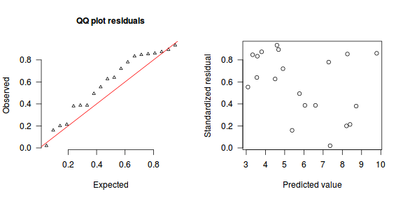
[1] 0.5533333 0.8466667 0.6400000 0.8333333 0.8733333 0.6266667 0.9333333 0.8933333 0.7200000 0.1600000 0.4933333 0.3866667 0.3866667 0.7800000 0.0200000 0.2000000 0.8533333 0.2133333 0.3800000 0.8600000
Although there is a slight hint of non-linearity in that the residuals are high for low and high fitted values and lower in the middle, this might well be an artifact of the small data set size. By change, most of the observed values in the middle range of the predictor were zero.
Exploring the model parameters, inference
If there was any evidence that the assumptions had been violated or the model was not an appropriate fit, then we would need to reconsider the model and start the process again. In this case, there is no evidence that the test will be unreliable so we can proceed to explore the test statistics.
As with most Bayesian models, it is best to base conclusions on medians rather than means.
print(dat.zinb.jags)
Inference for Bugs model at "5", fit using jags, 3 chains, each with 1e+05 iterations (first 50000 discarded), n.thin = 50 n.sims = 3000 iterations saved mu.vect sd.vect 2.5% 25% 50% 75% 97.5% Rhat n.eff beta0 0.973 0.453 0.058 0.679 0.961 1.269 1.882 1.001 3000 beta1 0.066 0.042 -0.014 0.037 0.065 0.094 0.151 1.001 3000 gamma -0.210 0.462 -1.133 -0.521 -0.202 0.090 0.674 1.002 1200 psi 0.450 0.109 0.244 0.373 0.450 0.522 0.662 1.003 1000 theta 2.190 0.363 1.724 1.939 2.102 2.360 3.133 1.001 3000 deviance 82.759 2.824 79.157 80.658 82.132 84.199 89.605 1.001 3000 For each parameter, n.eff is a crude measure of effective sample size, and Rhat is the potential scale reduction factor (at convergence, Rhat=1). DIC info (using the rule, pD = var(deviance)/2) pD = 4.0 and DIC = 86.7 DIC is an estimate of expected predictive error (lower deviance is better).library(plyr) adply(dat.zinb.jags$BUGSoutput$sims.matrix, 2, function(x) { data.frame(Median=median(x), Mean=mean(x), HPDinterval(as.mcmc(x)), HPDinterval(as.mcmc(x),p=0.5)) })
X1 Median Mean lower upper lower.1 upper.1 1 beta0 0.96103123 0.97276291 0.13961096 1.9515909 0.66801095 1.25524602 2 beta1 0.06467899 0.06570763 -0.01525967 0.1486955 0.03618379 0.09232641 3 deviance 82.13216622 82.75885652 78.74846503 88.3394029 79.66753681 82.68026059 4 gamma -0.20172349 -0.21028082 -1.12438237 0.6754259 -0.52792406 0.07915285 5 psi 0.44973945 0.45021792 0.24269534 0.6600966 0.37100120 0.51977789 6 theta 2.10185552 2.18996772 1.62902894 2.9316514 1.83725582 2.19604146
Actually, many find it more palatable to express the estimates in the original scale of the observations rather than on a log scale.
library(plyr) adply(exp(dat.zinb.jags$BUGSoutput$sims.matrix[,1:2]), 2, function(x) { data.frame(Median=median(x), Mean=mean(x), HPDinterval(as.mcmc(x)), HPDinterval(as.mcmc(x),p=0.5)) })
X1 Median Mean lower upper lower.1 upper.1 1 beta0 2.614391 2.933031 0.8237093 5.78519 1.615310 3.052375 2 beta1 1.066817 1.068866 0.9848562 1.16032 1.034969 1.094738
Conclusions: We would reject the null hypothesis of no effect of $x$ on $y$. An increase in x is associated with a significant linear increase (positive slope) in the abundance of $y$. Every 1 unit increase in $x$ results in a log
0.064679unit increase in $y$. We usually express this in terms of abundance rather than log abundance, so every 1 unit increase in $x$ results in a (e^{0.064679}=1.0668165)1.0668165unit increase in the abundance of $y$.Further explorations of the trends
A measure of the strength of the relationship can be obtained according to: $$R^2 = 1 - \frac{RSS_{model}}{RSS_{null}}$$
Alternatively, we could use McFadden's psuedo $$R^2 = 1-\frac{\mathcal{LL}(Model_{full})}{\mathcal{LL}(Model_{reduced})}$$ [[http://www.statisticalhorizons.com/category/uncategorized]] - about a quarter of the way down the page.
Xmat <- model.matrix(~x, dat=dat.zinb) #expected values on a log scale neta<-coefs %*% t(Xmat) #expected value on response scale eta <- exp(neta) lambda <- sweep(eta,2,ifelse(dat.zinb$y==0,0,1),'*') expY <- sweep(lambda,2,1-theta,'*') #calculate the raw SS residuals SSres <- apply((-1*(sweep(expY,2,dat.zinb$y,'-')))^2,1,sum) SSres.null <- sum((dat.zinb$y - mean(dat.zinb$y))^2) #calculate the model r2 1-mean(SSres)/SSres.null
[1] 0.3869893
Conclusions:
38.7% of the variation in $y$ abundance can be explained by its relationship with $x$.
Worked Examples
Basic χ2 references
- Logan (2010) - Chpt 16-17
- Quinn & Keough (2002) - Chpt 13-14
Poisson t-test
A marine ecologist was interested in examining the effects of wave exposure on the abundance of the striped limpet Siphonaria diemenensis on rocky intertidal shores. To do so, a single quadrat was placed on 10 exposed (to large waves) shores and 10 sheltered shores. From each quadrat, the number of Siphonaria diemenensis were counted.
Download Limpets data setFormat of limpets.csv data files Count Shore 1 sheltered 3 sheltered 2 sheltered 1 sheltered 4 sheltered ... ... Shore Categorical description of the shore type (sheltered or exposed) - Predictor variable Count Number of limpets per quadrat - Response variable 
Open the limpet data set.
Show codelimpets <- read.table('../downloads/data/limpets.csv', header=T, sep=',', strip.white=T) limpets
Count Shore 1 2 sheltered 2 2 sheltered 3 0 sheltered 4 6 sheltered 5 0 sheltered 6 3 sheltered 7 3 sheltered 8 0 sheltered 9 1 sheltered 10 2 sheltered 11 5 exposed 12 3 exposed 13 6 exposed 14 3 exposed 15 4 exposed 16 7 exposed 17 10 exposed 18 3 exposed 19 5 exposed 20 2 exposed
-
Is there any evidence that these assumptions have been violated?
Show codeboxplot(Count~Shore, data=limpets)
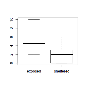
library(vcd) fit <- goodfit(limpets$Count, type='poisson') summary(fit)
Goodness-of-fit test for poisson distribution X^2 df P(> X^2) Likelihood Ratio 14.03661 7 0.05053407rootogram(fit)
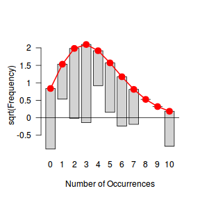
fit <- goodfit(limpets$Count, type='nbinom') summary(fit)
Goodness-of-fit test for nbinomial distribution X^2 df P(> X^2) Likelihood Ratio 9.105475 6 0.1677325rootogram(fit)
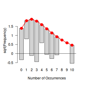
Ord_plot(limpets$Count, tol=0.2)
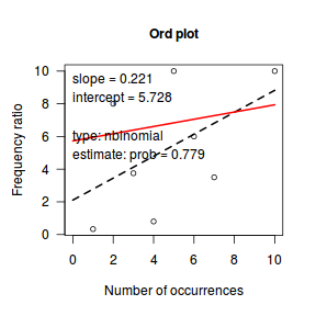
distplot(limpets$Count, type='poisson')
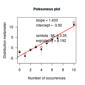
## Although we could argue that NB more appropriate than Poisson, this is possibly ## due to the small sample size. Small samples are more varied than the populations ## from which they are drawn
- The assumption of normality has been violated?
- The assumption of homogeneity of variance has been violated?
- Notwithstanding the very small sample size, is a Poisson distribution appropriate?
- The assumption of normality has been violated?
- Lets instead we fit the same model with a Poisson distribution.
$$
\begin{align}
Y_i&\sim{}P(\lambda) & (\text{response distribution})\\
log(\lambda_i)&=\eta_i & (\text{link function})\\
\eta_i&=\beta_0+\beta_1 X_i & (\text{linear predictor})\\
\beta_0, \beta_1&\sim{}\mathcal{N}(0,100) & (\text{week Bayesian prior})\\
\end{align}
$$
Show BRMS code
limpets.brm <- brm(Count~Shore, family=poisson, data=limpets, prior = c(set_prior("normal(0,100)", class="Intercept"), set_prior("normal(0,100)", class="b")), chains=3, iter=2000, warmup=1000, thin=2)
SAMPLING FOR MODEL 'poisson(log) brms-model' NOW (CHAIN 1). Chain 1, Iteration: 1 / 2000 [ 0%] (Warmup) Chain 1, Iteration: 200 / 2000 [ 10%] (Warmup) Chain 1, Iteration: 400 / 2000 [ 20%] (Warmup) Chain 1, Iteration: 600 / 2000 [ 30%] (Warmup) Chain 1, Iteration: 800 / 2000 [ 40%] (Warmup) Chain 1, Iteration: 1000 / 2000 [ 50%] (Warmup) Chain 1, Iteration: 1001 / 2000 [ 50%] (Sampling) Chain 1, Iteration: 1200 / 2000 [ 60%] (Sampling) Chain 1, Iteration: 1400 / 2000 [ 70%] (Sampling) Chain 1, Iteration: 1600 / 2000 [ 80%] (Sampling) Chain 1, Iteration: 1800 / 2000 [ 90%] (Sampling) Chain 1, Iteration: 2000 / 2000 [100%] (Sampling)# # Elapsed Time: 0.037372 seconds (Warm-up) # 0.036072 seconds (Sampling) # 0.073444 seconds (Total) # SAMPLING FOR MODEL 'poisson(log) brms-model' NOW (CHAIN 2). Chain 2, Iteration: 1 / 2000 [ 0%] (Warmup) Chain 2, Iteration: 200 / 2000 [ 10%] (Warmup) Chain 2, Iteration: 400 / 2000 [ 20%] (Warmup) Chain 2, Iteration: 600 / 2000 [ 30%] (Warmup) Chain 2, Iteration: 800 / 2000 [ 40%] (Warmup) Chain 2, Iteration: 1000 / 2000 [ 50%] (Warmup) Chain 2, Iteration: 1001 / 2000 [ 50%] (Sampling) Chain 2, Iteration: 1200 / 2000 [ 60%] (Sampling) Chain 2, Iteration: 1400 / 2000 [ 70%] (Sampling) Chain 2, Iteration: 1600 / 2000 [ 80%] (Sampling) Chain 2, Iteration: 1800 / 2000 [ 90%] (Sampling) Chain 2, Iteration: 2000 / 2000 [100%] (Sampling)# # Elapsed Time: 0.038755 seconds (Warm-up) # 0.038426 seconds (Sampling) # 0.077181 seconds (Total) # SAMPLING FOR MODEL 'poisson(log) brms-model' NOW (CHAIN 3). Chain 3, Iteration: 1 / 2000 [ 0%] (Warmup) Chain 3, Iteration: 200 / 2000 [ 10%] (Warmup) Chain 3, Iteration: 400 / 2000 [ 20%] (Warmup) Chain 3, Iteration: 600 / 2000 [ 30%] (Warmup) Chain 3, Iteration: 800 / 2000 [ 40%] (Warmup) Chain 3, Iteration: 1000 / 2000 [ 50%] (Warmup) Chain 3, Iteration: 1001 / 2000 [ 50%] (Sampling) Chain 3, Iteration: 1200 / 2000 [ 60%] (Sampling) Chain 3, Iteration: 1400 / 2000 [ 70%] (Sampling) Chain 3, Iteration: 1600 / 2000 [ 80%] (Sampling) Chain 3, Iteration: 1800 / 2000 [ 90%] (Sampling) Chain 3, Iteration: 2000 / 2000 [100%] (Sampling)# # Elapsed Time: 0.045705 seconds (Warm-up) # 0.038072 seconds (Sampling) # 0.083777 seconds (Total) #
- Explore the chain mixing diagnostics.
- Trace plots
Show code
library(gridExtra) grid.arrange(stan_trace(limpets.brm$fit, ncol=1), stan_dens(limpets.brm$fit, separate_chains=TRUE,ncol=1), ncol=2)
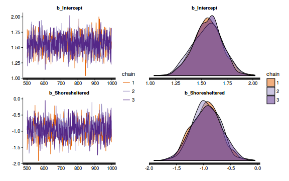
- Autocorrelation
Show code
stan_ac(limpets.brm$fit)
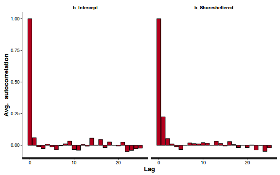
- Step size characteristics (STAN only)
Show code
summary(do.call(rbind, args = get_sampler_params(limpets.brm$fit, inc_warmup = FALSE)), digits = 2)
accept_stat__ stepsize__ treedepth__ n_leapfrog__ n_divergent__ Min. :0.28 Min. :0.60 Min. :1.0 Min. :1.0 Min. :0 1st Qu.:0.91 1st Qu.:0.60 1st Qu.:2.0 1st Qu.:3.0 1st Qu.:0 Median :0.97 Median :0.74 Median :2.0 Median :3.0 Median :0 Mean :0.93 Mean :0.70 Mean :2.2 Mean :3.8 Mean :0 3rd Qu.:1.00 3rd Qu.:0.76 3rd Qu.:3.0 3rd Qu.:5.0 3rd Qu.:0 Max. :1.00 Max. :0.76 Max. :3.0 Max. :7.0 Max. :0
stan_diag(limpets.brm$fit)
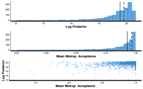
stan_diag(limpets.brm$fit, information = "stepsize")
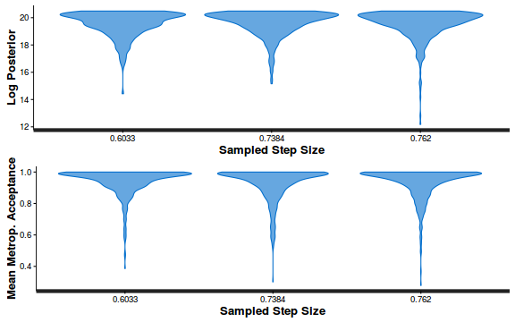
stan_diag(limpets.brm$fit, information = "treedepth")
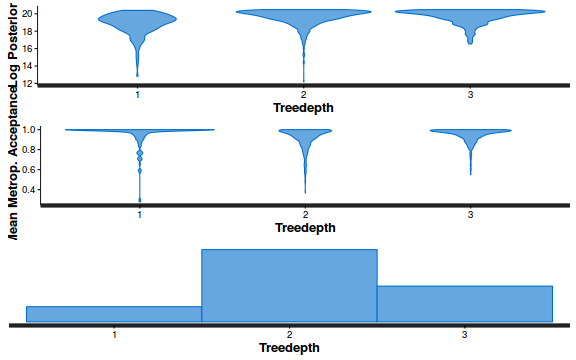
stan_diag(limpets.brm$fit, information = "divergence")
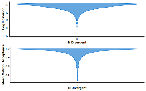
library(gridExtra) grid.arrange(stan_rhat(limpets.brm$fit) + theme_classic(8), stan_ess(limpets.brm$fit) + theme_classic(8), stan_mcse(limpets.brm$fit) + theme_classic(8), ncol = 2)
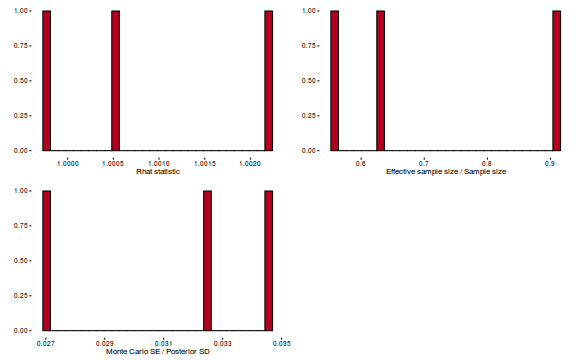
- Trace plots
- Explore the model fit diagnostics.
- Explore the patterns in simulated residuals:
Show code
lambda.brm = fitted(limpets.brm, scale='response', summary=FALSE) simRes <- function(lambda, Y,n=250, plot=T, family='negbin', size=NULL,theta=NULL) { require(gap) N = length(Y) sim = switch(family, 'poisson' = matrix(rpois(n*N,apply(lambda,2,mean)),ncol=N, byrow=TRUE), 'negbin' = matrix(MASS:::rnegbin(n*N,apply(lambda,2,mean),size),ncol=N, byrow=TRUE), 'zip' = matrix(gamlss.dist:::rZIP(n*N,apply(lambda,2,mean),theta),ncol=N, byrow=TRUE), 'zinb' = matrix(gamlss.dist:::rZINBI(n*N,apply(lambda,2,mean),sigma=theta,nu=size),ncol=N, byrow=TRUE) ) a = apply(sim + runif(n,-0.5,0.5),2,ecdf) resid<-NULL for (i in 1:length(Y)) resid<-c(resid,a[[i]](Y[i] + runif(1 ,-0.5,0.5))) if (plot==T) { par(mfrow=c(1,2)) gap::qqunif(resid,pch = 2, bty = "n", logscale = F, col = "black", cex = 0.6, main = "QQ plot residuals", cex.main = 1, las=1) plot(resid~apply(lambda,2,mean), xlab='Predicted value', ylab='Standardized residual', las=1) } resid } simRes(lambda.brm, limpets$Count, family='poisson')
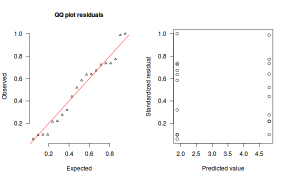
[1] 0.636 0.584 0.060 1.000 0.096 0.724 0.736 0.100 0.320 0.672 0.640 0.276 0.736 0.220 0.440 0.772 0.988 0.216 0.520 0.100
- Goodness of fit test:
Show code
Resid.brm <- residuals(limpets.brm, type='pearson', summary=FALSE) SSres.brm <- apply(Resid.brm^2,1,sum) lambda.brm = fitted(limpets.brm, scale='response', summary=FALSE) YNew.brm <- matrix(rpois(length(lambda.brm), lambda=lambda.brm),nrow=nrow(lambda.brm)) Resid1.brm<-(lambda.brm - YNew.brm)/sqrt(lambda.brm) SSres.sim.brm<-apply(Resid1.brm^2,1,sum) mean(SSres.sim.brm>SSres.brm)
[1] 0.1686667
- Fitted and observed values (plot):
Show code
newdata <- data.frame(Shore=levels(limpets$Shore)) tempdata = fitted(limpets.brm, scale='response',newdata=newdata) tempdata <- cbind(newdata, Mean=tempdata[,'Estimate'], Lower=tempdata[,'2.5%ile'], Upper=tempdata[,'97.5%ile']) tempdata
Shore Mean Lower Upper 1 exposed 4.808977 3.582597 6.194391 2 sheltered 1.891051 1.172518 2.870922
library(ggplot2) ggplot(limpets, aes(y=Count, x=Shore)) + geom_boxplot() + geom_pointrange(data=tempdata,aes(y=Mean, ymin=Lower, ymax=Upper), color='red')

##OR the manual way Xmat <- model.matrix(~Shore, data=newdata) coefs <- as.matrix(as.data.frame(rstan:::extract(limpets.brm$fit)))[,1:2] fit = exp(coefs %*% t(Xmat)) tempdata <- cbind(newdata, plyr:::adply(fit, 2, function(x) { data.frame(Mean=mean(x), Median=median(x), HPDinterval(as.mcmc(x))) })) ggplot(limpets, aes(y=Count, x=Shore)) + geom_boxplot() + geom_pointrange(data=tempdata,aes(y=Mean, ymin=lower, ymax=upper), color='red')
- Check for overdispersion:
Show code
coefs <- as.matrix(as.data.frame(rstan:::extract(limpets.brm$fit)))[,1:2] Resid <- residuals(limpets.brm, type='pearson',summary=FALSE) RSS <- apply(Resid^2,1,sum) Disp <- RSS/(nrow(limpets)-ncol(coefs)) data.frame(Median=median(Disp), Mean=mean(Disp), HPDinterval(as.mcmc(Disp)))
Median Mean lower upper var1 1.384552 1.415549 1.319196 1.619498
- Explore the patterns in simulated residuals:
- Explore the parameter estimates
Show code
summary(limpets.brm)
Family: poisson (log) Formula: Count ~ Shore Data: limpets (Number of observations: 20) Samples: 3 chains, each with iter = 2000; warmup = 1000; thin = 2; total post-warmup samples = 1500 WAIC: Not computed Fixed Effects: Estimate Est.Error l-95% CI u-95% CI Eff.Sample Rhat Intercept 1.56 0.14 1.28 1.82 1361 1 Shoresheltered -0.95 0.26 -1.45 -0.43 952 1 Samples were drawn using sampling(NUTS). For each parameter, Eff.Sample is a crude measure of effective sample size, and Rhat is the potential scale reduction factor on split chains (at convergence, Rhat = 1).exp(coef(limpets.brm))
mean Intercept 4.761504 Shoresheltered 0.387136
coefs.brm <- as.matrix(as.data.frame(rstan:::extract(limpets.brm$fit))) coefs.brm <- coefs.brm[,grep('b', colnames(coefs.brm))] plyr:::adply(exp(coefs.brm), 2, function(x) { data.frame(Mean=mean(x), median=median(x), HPDinterval(as.mcmc(x))) })
X1 Mean median lower upper 1 b_Intercept 4.8089767 4.7877066 3.4711793 6.0637796 2 b_Shoresheltered 0.4008196 0.3880695 0.2186746 0.6188941
marginal_effects(limpets.brm)
- Estimate the strength of the relationship
Show code
## calculate the expected values on the response scale lambda.brm = fitted(limpets.brm, scale='response', summary=FALSE) ## calculate the raw SSresid SSres.brm <- apply((-1*(sweep(lambda.brm,2,limpets$Count,'-')))^2,1,sum) SSres.null <- sum((limpets$Count - mean(limpets$Count))^2) #OR #calculate the model r2 1-mean(SSres.brm)/SSres.null
[1] 0.2857745
#OR manually coefs <- as.matrix(as.data.frame(rstan:::extract(limpets.brm$fit))) coefs <- coefs.brm[,grep('b', colnames(coefs))] Xmat <- model.matrix(~Shore, data=limpets) lambda.brm = exp(coefs %*% t(Xmat)) ## calculate the raw SSresid SSres.brm <- apply((-1*(sweep(lambda.brm,2,limpets$Count,'-')))^2,1,sum) SSres.null <- crossprod(limpets$Count - mean(limpets$Count)) #calculate the model r2 1-mean(SSres.brm)/SSres.null
[,1] [1,] 0.2857745
## Alternatively.. R.var = apply(residuals(limpets.brm, summary=FALSE),1,var) X.var = apply(fitted(limpets.brm, summary=FALSE),1,var) R2.marginal <- X.var/(X.var + R.var) data.frame(Median=median(R2.marginal), coda:::HPDinterval(as.mcmc(R2.marginal)))
Median lower upper var1 0.3386231 0.1113502 0.5261667
- Construct a summary plot
Show code
newdata=data.frame(Shore=levels(limpets$Shore)) coefs <- as.matrix(as.data.frame(rstan:::extract(limpets.brm$fit))) coefs <- coefs.brm[,grep('b', colnames(coefs))] Xmat <- model.matrix(~Shore, data=newdata) fit = exp(coefs %*% t(Xmat)) newdata = cbind(newdata, plyr:::adply(fit, 2, function(x) { data.frame(Mean=mean(x), median=median(x), HPDinterval(as.mcmc(x))) })) ggplot(limpets, aes(y=Count, x=Shore)) + geom_point(color='grey') + geom_pointrange(data=newdata, aes(y=Mean, ymin=lower, ymax=upper)) + scale_y_continuous('Abundance of limpets') + scale_x_discrete('Shore type', breaks=c('exposed','sheltered'), labels=c('Exposed','Sheltered')) + theme_classic() + theme(axis.line.x=element_line(), axis.line.y=element_line())
At this point we could transform the data in an attempt to satisfy normality and homogeneity of variance. However, the analyses are then not on the scale of the data and thus the conclusions also pertain to a different scale. Furthermore, linear modelling on transformed count data is generally not as effective as modelling count data with a Poisson distribution.
Poisson ANOVA (regression)
We once again return to a modified example from Quinn and Keough (2002). In Exercise 1 of Workshop 9.4a, we introduced an experiment by Day and Quinn (1989) that examined how rock surface type affected the recruitment of barnacles to a rocky shore. The experiment had a single factor, surface type, with 4 treatments or levels: algal species 1 (ALG1), algal species 2 (ALG2), naturally bare surfaces (NB) and artificially scraped bare surfaces (S). There were 5 replicate plots for each surface type and the response (dependent) variable was the number of newly recruited barnacles on each plot after 4 weeks.
Download Day data set
Open the day data file.Format of day.csv data files TREAT BARNACLE ALG1 27 .. .. ALG2 24 .. .. NB 9 .. .. S 12 .. .. TREAT Categorical listing of surface types. ALG1 = algal species 1, ALG2 = algal species 2, NB = naturally bare surface, S = scraped bare surface. BARNACLE The number of newly recruited barnacles on each plot after 4 weeks.  Show code
day <- read.table('../downloads/data/day.csv', header=T, sep=',', strip.white=T) head(day)
TREAT BARNACLE 1 ALG1 27 2 ALG1 19 3 ALG1 18 4 ALG1 23 5 ALG1 25 6 ALG2 24
We previously analysed these data with via a classic linear model (ANOVA) as the data appeared to conform to the linear model assumptions. Alternatively, we could analyse these data with a generalized linear model (Poisson error distribution). Note that as the boxplots were all fairly symmetrical and equally varied, and the sample means are well away from zero (in fact there are no zero's in the data) we might suspect that whether we fit the model as a linear or generalized linear model is probably not going to be of great consequence. Nevertheless, it does then provide a good comparison between the two frameworks.
-
Using boxplots re-examine the assumptions of normality and homogeneity of variance.
Note that when sample sizes are small (as is the case with this data set), these ANOVA assumptions cannot reliably be checked using boxplots since boxplots require at least 5 replicates (and preferably more), from which to calculate the median and quartiles.
As with regression analysis, it is the assumption of homogeneity of variances (and in particular, whether there is a relationship between the mean and variance) that is of most concern for ANOVA.
Show code
boxplot(BARNACLE~TREAT, data=day)
library(vcd) fit <- goodfit(day$BARNACLE, type='poisson') summary(fit)
Goodness-of-fit test for poisson distribution X^2 df P(> X^2) Likelihood Ratio 32.19209 17 0.01424181rootogram(fit)
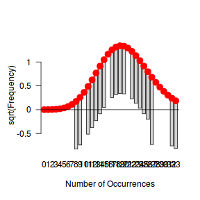
fit <- goodfit(day$BARNACLE, type='nbinom') summary(fit)
Goodness-of-fit test for nbinomial distribution X^2 df P(> X^2) Likelihood Ratio 18.41836 16 0.2999741rootogram(fit)
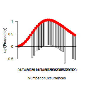
distplot(day$BARNACLE, type='poisson')
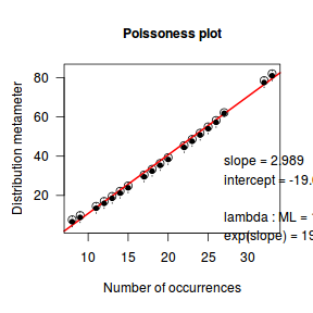
## Poisson would appear appropriate - Fit the generalized linear model (GLM) relating the number of newly recruited barnacles to substrate type.
$$
\begin{align}
Y_i&\sim{}P(\lambda) & (\text{response distribution})\\
log(\lambda_i)&=\eta_i & (\text{link function})\\
\eta_i&=\beta_0+\beta_1 X_i & (\text{linear predictor})\\
\beta_0, \beta_1&\sim{}\mathcal{N}(0,1000) & (\text{week Bayesian prior})\\
\end{align}
$$
Show BRMS code
day.brm <- brm(BARNACLE~TREAT, family=poisson, data=day, prior = c(set_prior("normal(0,1000)", class="Intercept"), set_prior("normal(0,1000)", class="b")), chains=3, iter=2000, warmup=1000, thin=2)
SAMPLING FOR MODEL 'poisson(log) brms-model' NOW (CHAIN 1). Chain 1, Iteration: 1 / 2000 [ 0%] (Warmup) Chain 1, Iteration: 200 / 2000 [ 10%] (Warmup) Chain 1, Iteration: 400 / 2000 [ 20%] (Warmup) Chain 1, Iteration: 600 / 2000 [ 30%] (Warmup) Chain 1, Iteration: 800 / 2000 [ 40%] (Warmup) Chain 1, Iteration: 1000 / 2000 [ 50%] (Warmup) Chain 1, Iteration: 1001 / 2000 [ 50%] (Sampling) Chain 1, Iteration: 1200 / 2000 [ 60%] (Sampling) Chain 1, Iteration: 1400 / 2000 [ 70%] (Sampling) Chain 1, Iteration: 1600 / 2000 [ 80%] (Sampling) Chain 1, Iteration: 1800 / 2000 [ 90%] (Sampling) Chain 1, Iteration: 2000 / 2000 [100%] (Sampling)# # Elapsed Time: 0.04357 seconds (Warm-up) # 0.041621 seconds (Sampling) # 0.085191 seconds (Total) # SAMPLING FOR MODEL 'poisson(log) brms-model' NOW (CHAIN 2). Chain 2, Iteration: 1 / 2000 [ 0%] (Warmup) Chain 2, Iteration: 200 / 2000 [ 10%] (Warmup) Chain 2, Iteration: 400 / 2000 [ 20%] (Warmup) Chain 2, Iteration: 600 / 2000 [ 30%] (Warmup) Chain 2, Iteration: 800 / 2000 [ 40%] (Warmup) Chain 2, Iteration: 1000 / 2000 [ 50%] (Warmup) Chain 2, Iteration: 1001 / 2000 [ 50%] (Sampling) Chain 2, Iteration: 1200 / 2000 [ 60%] (Sampling) Chain 2, Iteration: 1400 / 2000 [ 70%] (Sampling) Chain 2, Iteration: 1600 / 2000 [ 80%] (Sampling) Chain 2, Iteration: 1800 / 2000 [ 90%] (Sampling) Chain 2, Iteration: 2000 / 2000 [100%] (Sampling)# # Elapsed Time: 0.055115 seconds (Warm-up) # 0.04102 seconds (Sampling) # 0.096135 seconds (Total) # SAMPLING FOR MODEL 'poisson(log) brms-model' NOW (CHAIN 3). Chain 3, Iteration: 1 / 2000 [ 0%] (Warmup) Chain 3, Iteration: 200 / 2000 [ 10%] (Warmup) Chain 3, Iteration: 400 / 2000 [ 20%] (Warmup) Chain 3, Iteration: 600 / 2000 [ 30%] (Warmup) Chain 3, Iteration: 800 / 2000 [ 40%] (Warmup) Chain 3, Iteration: 1000 / 2000 [ 50%] (Warmup) Chain 3, Iteration: 1001 / 2000 [ 50%] (Sampling) Chain 3, Iteration: 1200 / 2000 [ 60%] (Sampling) Chain 3, Iteration: 1400 / 2000 [ 70%] (Sampling) Chain 3, Iteration: 1600 / 2000 [ 80%] (Sampling) Chain 3, Iteration: 1800 / 2000 [ 90%] (Sampling) Chain 3, Iteration: 2000 / 2000 [100%] (Sampling)# # Elapsed Time: 0.052148 seconds (Warm-up) # 0.045466 seconds (Sampling) # 0.097614 seconds (Total) #
- Explore the chain mixing diagnostics.
- Trace plots
Show code
library(gridExtra) grid.arrange(stan_trace(day.brm$fit, ncol=1), stan_dens(day.brm$fit, separate_chains=TRUE,ncol=1), ncol=2)
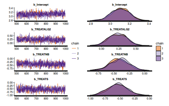
- Autocorrelation
Show code
stan_ac(day.brm$fit)
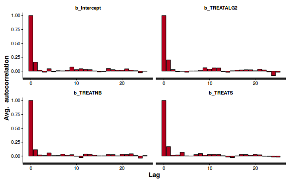
- Step size characteristics (STAN only)
Show code
summary(do.call(rbind, args = get_sampler_params(day.brm$fit, inc_warmup = FALSE)), digits = 2)
accept_stat__ stepsize__ treedepth__ n_leapfrog__ n_divergent__ Min. :0.17 Min. :0.62 Min. :1.0 Min. :1.0 Min. :0 1st Qu.:0.86 1st Qu.:0.62 1st Qu.:2.0 1st Qu.:3.0 1st Qu.:0 Median :0.95 Median :0.64 Median :2.0 Median :3.0 Median :0 Mean :0.91 Mean :0.64 Mean :2.4 Mean :4.5 Mean :0 3rd Qu.:0.99 3rd Qu.:0.66 3rd Qu.:3.0 3rd Qu.:7.0 3rd Qu.:0 Max. :1.00 Max. :0.66 Max. :3.0 Max. :7.0 Max. :0
stan_diag(day.brm$fit)
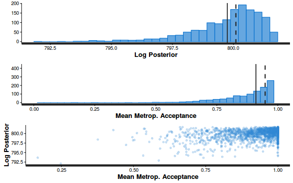
stan_diag(day.brm$fit, information = "stepsize")
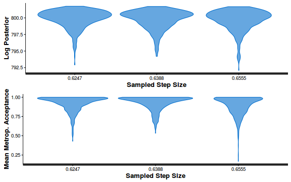
stan_diag(day.brm$fit, information = "treedepth")
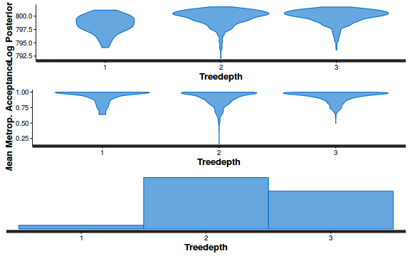
stan_diag(day.brm$fit, information = "divergence")
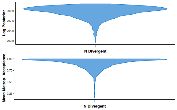
library(gridExtra) grid.arrange(stan_rhat(day.brm$fit) + theme_classic(8), stan_ess(day.brm$fit) + theme_classic(8), stan_mcse(day.brm$fit) + theme_classic(8), ncol = 2)
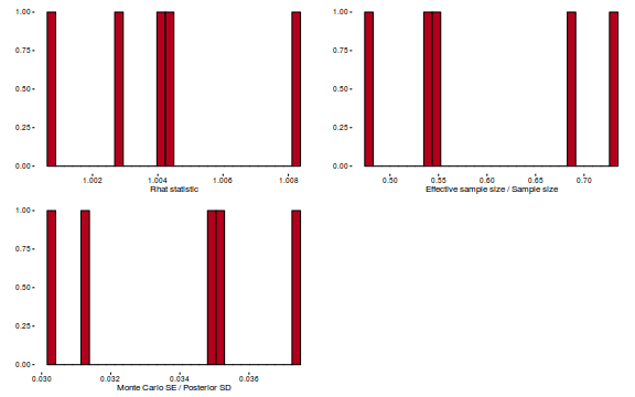
- Trace plots
- Explore the model fit diagnostics.
- Explore the patterns in simulated residuals:
Show code
lambda.brm = fitted(day.brm, scale='response', summary=FALSE) simRes <- function(lambda, Y,n=250, plot=T, family='negbin', size=NULL,theta=NULL) { require(gap) N = length(Y) sim = switch(family, 'poisson' = matrix(rpois(n*N,apply(lambda,2,mean)),ncol=N, byrow=TRUE), 'negbin' = matrix(MASS:::rnegbin(n*N,apply(lambda,2,mean),size),ncol=N, byrow=TRUE), 'zip' = matrix(gamlss.dist:::rZIP(n*N,apply(lambda,2,mean),theta),ncol=N, byrow=TRUE), 'zinb' = matrix(gamlss.dist:::rZINBI(n*N,apply(lambda,2,mean),sigma=theta,nu=size),ncol=N, byrow=TRUE) ) a = apply(sim + runif(n,-0.5,0.5),2,ecdf) resid<-NULL for (i in 1:length(Y)) resid<-c(resid,a[[i]](Y[i] + runif(1 ,-0.5,0.5))) if (plot==T) { par(mfrow=c(1,2)) gap::qqunif(resid,pch = 2, bty = "n", logscale = F, col = "black", cex = 0.6, main = "QQ plot residuals", cex.main = 1, las=1) plot(resid~apply(lambda,2,mean), xlab='Predicted value', ylab='Standardized residual', las=1) } resid } simRes(lambda.brm, day$BARNACLE, family='poisson')
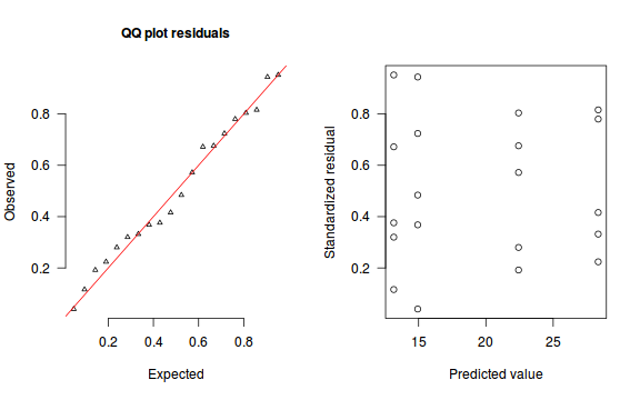
[1] 0.804 0.280 0.192 0.572 0.676 0.224 0.816 0.416 0.332 0.780 0.040 0.368 0.724 0.484 0.944 0.376 0.116 0.672 0.952 0.320
- Goodness of fit test:
Show code
Resid.brm <- residuals(day.brm, type='pearson', summary=FALSE) SSres.brm <- apply(Resid.brm^2,1,sum) lambda.brm = fitted(day.brm, scale='response', summary=FALSE) YNew.brm <- matrix(rpois(length(lambda.brm), lambda=lambda.brm),nrow=nrow(lambda.brm)) Resid1.brm<-(lambda.brm - YNew.brm)/sqrt(lambda.brm) SSres.sim.brm<-apply(Resid1.brm^2,1,sum) mean(SSres.sim.brm>SSres.brm)
[1] 0.5986667
- Fitted and observed values (plot):
Show code
newdata <- data.frame(TREAT=levels(day$TREAT)) tempdata = fitted(day.brm, scale='response',newdata=newdata) tempdata <- cbind(newdata, Mean=tempdata[,'Estimate'], Lower=tempdata[,'2.5%ile'], Upper=tempdata[,'97.5%ile']) tempdata
TREAT Mean Lower Upper 1 ALG1 22.42653 18.50291 26.69970 2 ALG2 28.34577 23.75776 33.21707 3 NB 14.93645 11.56363 18.37661 4 S 13.15741 10.15435 16.54420
library(ggplot2) ggplot(day, aes(y=BARNACLE, x=TREAT)) + geom_boxplot() + geom_pointrange(data=tempdata,aes(y=Mean, ymin=Lower, ymax=Upper), color='red')

##OR the manual way Xmat <- model.matrix(~TREAT, data=newdata) coefs <- as.matrix(as.data.frame(rstan:::extract(day.brm$fit))) coefs <- coefs[,grep('^b_', colnames(coefs))] fit = exp(coefs %*% t(Xmat)) tempdata <- cbind(newdata, plyr:::adply(fit, 2, function(x) { data.frame(Mean=mean(x), Median=median(x), HPDinterval(as.mcmc(x))) })) ggplot(day, aes(y=BARNACLE, x=TREAT)) + geom_boxplot() + geom_pointrange(data=tempdata,aes(y=Mean, ymin=lower, ymax=upper), color='red')
- Check for overdispersion:
Show code
coefs <- as.matrix(as.data.frame(rstan:::extract(day.brm$fit))) coefs <- coefs[,grep('^b_', colnames(coefs))] Resid <- residuals(day.brm, type='pearson',summary=FALSE) RSS <- apply(Resid^2,1,sum) Disp <- RSS/(nrow(day)-ncol(coefs)) data.frame(Median=median(Disp), Mean=mean(Disp), HPDinterval(as.mcmc(Disp)))
Median Mean lower upper var1 1.072787 1.110258 0.9095692 1.39219
- Explore the patterns in simulated residuals:
- Explore the parameter estimates
Show code
summary(day.brm)
Family: poisson (log) Formula: BARNACLE ~ TREAT Data: day (Number of observations: 20) Samples: 3 chains, each with iter = 2000; warmup = 1000; thin = 2; total post-warmup samples = 1500 WAIC: Not computed Fixed Effects: Estimate Est.Error l-95% CI u-95% CI Eff.Sample Rhat Intercept 3.11 0.09 2.92 3.28 1099 1.00 TREATALG2 0.23 0.13 -0.01 0.48 1026 1.00 TREATNB -0.41 0.15 -0.72 -0.12 818 1.01 TREATS -0.54 0.16 -0.84 -0.22 721 1.00 Samples were drawn using sampling(NUTS). For each parameter, Eff.Sample is a crude measure of effective sample size, and Rhat is the potential scale reduction factor on split chains (at convergence, Rhat = 1).exp(coef(day.brm))
mean Intercept 22.3302880 TREATALG2 1.2647170 TREATNB 0.6643044 TREATS 0.5845021
coefs.brm <- as.matrix(as.data.frame(rstan:::extract(day.brm$fit))) coefs.brm <- coefs.brm[,grep('b', colnames(coefs.brm))] plyr:::adply(exp(coefs.brm), 2, function(x) { data.frame(Mean=mean(x), median=median(x), HPDinterval(as.mcmc(x))) })
X1 Mean median lower upper 1 b_Intercept 22.4265258 22.3563112 18.7801517 26.9246921 2 b_TREATALG2 1.2750621 1.2633289 0.9820844 1.5952722 3 b_TREATNB 0.6718217 0.6643929 0.4654365 0.8588770 4 b_TREATS 0.5919046 0.5845745 0.4160054 0.7742567
marginal_effects(day.brm)
- Estimate the strength of the relationship
Show code
## calculate the expected values on the response scale lambda.brm = fitted(day.brm, scale='response', summary=FALSE) ## calculate the raw SSresid SSres.brm <- apply((-1*(sweep(lambda.brm,2,day$BARNACLE,'-')))^2,1,sum) SSres.null <- sum((day$BARNACLE - mean(day$BARNACLE))^2) #OR #calculate the model r2 1-mean(SSres.brm)/SSres.null
[1] 0.635007
#OR manually coefs <- as.matrix(as.data.frame(rstan:::extract(day.brm$fit))) coefs <- coefs[,grep('b', colnames(coefs))] Xmat <- model.matrix(~TREAT, data=day) lambda.brm = exp(coefs %*% t(Xmat)) ## calculate the raw SSresid SSres.brm <- apply((-1*(sweep(lambda.brm,2,day$BARNACLE,'-')))^2,1,sum) SSres.null <- crossprod(day$BARNACLE - mean(day$BARNACLE)) #calculate the model r2 1-mean(SSres.brm)/SSres.null
[,1] [1,] 0.635007
## Alternatively.. R.var = apply(residuals(day.brm, summary=FALSE),1,var) X.var = apply(fitted(day.brm, summary=FALSE),1,var) R2.marginal <- X.var/(X.var + R.var) data.frame(Median=median(R2.marginal), coda:::HPDinterval(as.mcmc(R2.marginal)))
Median lower upper var1 0.6985856 0.5149793 0.7759515
- Although we have now established that there is a statistical difference between the group means,
we do not yet know which group(s) are different from which other(s).
To address this we can explore all pairwise contrasts from the posterior. Note, careful when back transforming from log.
Recall that log laws indicate that $log(a) - log(b) = log(a/b)$.
Show code
coefs <-as.matrix(as.data.frame(rstan:::extract(day.brm$fit))) coefs <- coefs[,grep('b_', colnames(coefs))] newdata <- data.frame(TREAT=levels(day$TREAT)) Xmat <- model.matrix(~TREAT, data=newdata) library(multcomp) tuk.mat <- contrMat(n=table(newdata$TREAT), type="Tukey") Xmat <- model.matrix(~TREAT, data=newdata) Xmat <- tuk.mat %*% Xmat fit <- exp(coefs %*% t(Xmat)) library(coda) MCMCsum <- function(x) { data.frame(Median=median(x, na.rm=TRUE), t(quantile(x,na.rm=TRUE)), HPDinterval(as.mcmc(x))) } plyr:::adply(as.matrix(fit),2,MCMCsum)
X1 Median X0. X25. X50. X75. X100. lower upper 1 ALG2 - ALG1 1.2633289 0.8452016 1.1549126 1.2633289 1.3888569 2.0054558 0.9820844 1.5952722 2 NB - ALG1 0.6643929 0.4142791 0.5990942 0.6643929 0.7348131 1.0752521 0.4654365 0.8588770 3 S - ALG1 0.5845745 0.3666083 0.5252027 0.5845745 0.6472396 0.9985889 0.4160054 0.7742567 4 NB - ALG2 0.5246730 0.3142344 0.4775387 0.5246730 0.5817067 0.8599918 0.3790918 0.6773199 5 S - ALG2 0.4627503 0.2666343 0.4155122 0.4627503 0.5136620 0.7633502 0.3366329 0.6175163 6 S - NB 0.8804989 0.5160321 0.7789036 0.8804989 0.9970252 1.6316219 0.6258814 1.2183909
## Due to log laws, these effects are multipliers rather than differences ## If you want to express the outcomes in terms of differences then it is necessary to ## estimate the cell posteriors and subtract those - this cannot easily be done Frequentist! Xmat <- model.matrix(~TREAT, data=newdata) fit <- exp(coefs %*% t(Xmat)) library(multcomp) tuk.mat <- contrMat(n=table(newdata$TREAT), type="Tukey") Xmat <- tuk.mat fit <- fit %*% t(Xmat) plyr:::adply(as.matrix(fit),2,MCMCsum)
X1 Median X0. X25. X50. X75. X100. lower upper 1 ALG2 - ALG1 5.895130 -3.772229 3.619496 5.895130 8.21805575 17.17097099 -0.03095788 12.031425 2 NB - ALG1 -7.483685 -16.063734 -9.424278 -7.483685 -5.67358521 1.43404144 -12.96977305 -2.324986 3 S - ALG1 -9.257110 -19.048803 -11.112041 -9.257110 -7.47521694 -0.02471089 -14.60523050 -4.132667 4 NB - ALG2 -13.383835 -25.127509 -15.420303 -13.383835 -11.30591077 -3.08899312 -19.21054550 -7.484513 5 S - ALG2 -15.182663 -26.816258 -17.194247 -15.182663 -13.16149810 -5.56128213 -20.74073778 -9.168501 6 S - NB -1.807393 -8.789820 -3.462725 -1.807393 -0.04160081 6.74548604 -6.36710762 2.861639
- Alternatively, it might be interesting to explore specific contrasts
- compare the two algal surfaces
- compare the two bare surfaces
- compare the algal and bare surfaces
Show code## Effect as a multiplier coefs <-as.matrix(as.data.frame(rstan:::extract(day.brm$fit))) coefs <- coefs[,grep('b_', colnames(coefs))] newdata <- data.frame(TREAT=levels(day$TREAT)) Xmat <- model.matrix(~TREAT, data=newdata) comp.mat <- rbind(c(1,-1,0,0), c(0,0,1,-1), c(1/2,1/2,-1/2,-1/2)) Xmat <- cbind(0,comp.mat %*% contr.treatment(4)) fit <- exp(coefs %*% t(Xmat)) MCMCsum <- function(x) { data.frame(Median=median(x, na.rm=TRUE), t(quantile(x,na.rm=TRUE)), HPDinterval(as.mcmc(x))) } plyr:::adply(as.matrix(fit),2,MCMCsum)
X1 Median X0. X25. X50. X75. X100. lower upper 1 1 0.7915595 0.4986398 0.7200166 0.7915595 0.8658664 1.183150 0.6083706 0.9906496 2 2 1.1357198 0.6128871 1.0029837 1.1357198 1.2838560 1.937864 0.7969842 1.5466949 3 3 1.8067288 1.2633552 1.6705385 1.8067288 1.9401542 2.563707 1.4381279 2.1821891
## Effect as a difference Xmat <- model.matrix(~TREAT, data=newdata) fit <- exp(coefs %*% t(Xmat)) comp.mat <- rbind(c(1,-1,0,0), c(0,0,1,-1), c(1/2,1/2,-1/2,-1/2)) fit <- fit %*% t(comp.mat) plyr:::adply(as.matrix(fit),2,MCMCsum)
X1 Median X0. X25. X50. X75. X100. lower upper 1 1 -5.895130 -17.170971 -8.21805575 -5.895130 -3.619496 3.772229 -12.031425 0.03095788 2 2 1.807393 -6.745486 0.04160081 1.807393 3.462725 8.789820 -2.861639 6.36710762 3 3 11.296350 4.225970 9.88922295 11.296350 12.684859 18.425620 7.272778 14.98168802
- Produce a suitable summary plot
Show code
coefs <-as.matrix(as.data.frame(rstan:::extract(day.brm$fit))) coefs <- coefs[,grep('b_', colnames(coefs))] newdata <- data.frame(TREAT=levels(day$TREAT)) Xmat <- model.matrix(~TREAT, data=newdata) fit = exp(coefs %*% t(Xmat)) newdata = cbind(newdata, plyr:::adply(fit, 2, function(x) { data.frame(Mean=mean(x, na.rm=TRUE),Median=median(x, na.rm=TRUE), HPDinterval(as.mcmc(x))) })) ggplot(day, aes(y=BARNACLE, x=TREAT)) + geom_point(color='grey') + geom_pointrange(data=newdata, aes(y=Mean, ymin=lower, ymax=upper)) + scale_y_continuous('Number of newly recruited Barnacles') + scale_x_discrete('Substrate type', breaks=c('ALG1','ALG2','NB','S'), labels=c('Algae 1','Algae 2', 'Naturally\nBare','Scraped\nBare')) + theme_classic() + theme(axis.line.x=element_line(), axis.line.y=element_line())
Poisson ANOVA (regression)
To investigate habitat differences in moth abundances, researchers from the Australian National University (ANU) in Canberra counted the number of individuals of two species of moth (recorded as A and P) along transects throughout a landscape comprising eight different habitat types ('Bank', 'Disturbed', 'Lowerside', 'NEsoak', 'NWsoak', 'SEsoak', 'SWsoak', 'Upperside'). For the data presented here, one of the habitat types ('Bank') has been ommitted as no moths were encounted in that habitat.
Although each transect was approximately the same length, each transect passed through multiple habitat types. Consequently, each transect was divided into sections according to habitat and the number of moths observed in each section recorded. Clearly, the number of observed moths in a section would be related to the length of the transect in that section. Therefore, the researchers also recorded the length of each habitat section.
Download moths data set
Open the day data file.Format of moth.csv data files METERS A P HABITAT 25 9 8 NWsoak 37 3 20 SWsoak 109 7 9 Lowerside 10 0 2 Lowerside 133 9 1 Upperside 26 3 18 Disturbed METERS The length of the section of transect A The number of moth species A observed in section of transect P The number of moth species P observed in section of transect HABITAT Categorical listing of the habitat type within section of transect.  Show code
moths <- read.csv('../downloads/data/moths.csv', header=T, strip.white=T) head(moths)
METERS A P HABITAT 1 25 9 8 NWsoak 2 37 3 20 SWsoak 3 109 7 9 Lowerside 4 10 0 2 Lowerside 5 133 9 1 Upperside 6 26 3 18 Disturbed
The primary focus of this question will be to investigate the effect of habitat on the abundance of moth species A.
- To standardize the moth counts for transect section length, we could convert the counts into densities (by dividing the A by METERS.
Create such as variable (DENSITY and explore the usual ANOVA assumptions.
Show code
moths <- within(moths, DENSITY<-A/METERS) boxplot(DENSITY~HABITAT, data=moths)
library(vcd) fit <- goodfit(moths$A, type='poisson') summary(fit)
Goodness-of-fit test for poisson distribution X^2 df P(> X^2) Likelihood Ratio 170.2708 11 1.037761e-30rootogram(fit)
fit <- goodfit(moths$A, type='nbinom') summary(fit)
Goodness-of-fit test for nbinomial distribution X^2 df P(> X^2) Likelihood Ratio 32.1636 10 0.0003760562rootogram(fit)
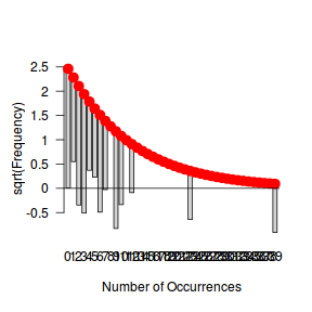
Ord_plot(moths$A, tol=0.2)
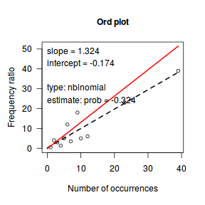
distplot(moths$A, type='poisson')
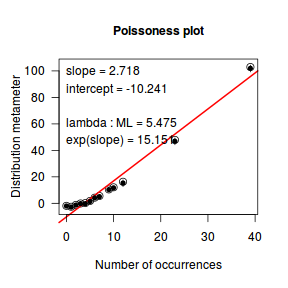
distplot(moths$A, type='nbinom')
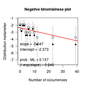
- Clearly, the there is an issue with normality and homogeneity of variance. Perhaps it would be worth transforming
density in an attempt to normalize these data. Given that there are densities of zero, a straight logarithmic transformation would not be appropriate.
Alternatives could inlude a square-root transform, a forth-root transform and a log plus 1 transform.
Show code
moths <- within(moths, DENSITY<-A/METERS) boxplot(sqrt(DENSITY)~HABITAT, data=moths)
boxplot((DENSITY)^0.25~HABITAT, data=moths)
boxplot(log(DENSITY+1)~HABITAT, data=moths)
- Arguably, non of the above transformations have improved the data's adherence to the linear modelling assumptions.
Count data (such as the abundance of moth species A) is unlikely to follow a normal or even log-normal distribution. Count data
are usually more appropriately modelled via a Poisson or Negative binomial distributions. Note, dividing by transect length is unlikely to alter
the underlying nature of the data distribution as it still based on counts.
Fit the generalized linear model (GLM) relating the number of moths to habitat.
$$
\begin{align}
Y_i&\sim{}P(\lambda) & (\text{response distribution})\\
log(\lambda_i)&=\eta_i & (\text{link function})\\
\eta_i&=\beta_0+\beta_1 X_i & (\text{linear predictor})\\
\beta_0, \beta_1&\sim{}\mathcal{N}(0,1000) & (\text{week Bayesian prior})\\
\end{align}
$$
OR
$$
\begin{align}
Y_i&\sim{}NB(p, size) & (\text{response distribution})\\
p &= size/(size + \lambda)\\
log(\lambda_i)&=\eta_i & (\text{link function})\\
\eta_i&=\beta_0+\beta_1 X_i & (\text{linear predictor})\\
\beta_0, \beta_1&\sim{}\mathcal{N}(0,1000) & (\text{week Bayesian prior})\\
size &\sim{}T3,0,5)& (\text{week student t prior})\\
\end{align}
$$
Show code
## Poisson model moths.brm <- brm(A~HABITAT, family=poisson, data=moths, prior = c(set_prior("normal(0,1000)", class="Intercept"), set_prior("normal(0,1000)", class="b")), chains=3, iter=2000, warmup=1000, thin=4)
SAMPLING FOR MODEL 'poisson(log) brms-model' NOW (CHAIN 1). Chain 1, Iteration: 1 / 2000 [ 0%] (Warmup) Chain 1, Iteration: 200 / 2000 [ 10%] (Warmup) Chain 1, Iteration: 400 / 2000 [ 20%] (Warmup) Chain 1, Iteration: 600 / 2000 [ 30%] (Warmup) Chain 1, Iteration: 800 / 2000 [ 40%] (Warmup) Chain 1, Iteration: 1000 / 2000 [ 50%] (Warmup) Chain 1, Iteration: 1001 / 2000 [ 50%] (Sampling) Chain 1, Iteration: 1200 / 2000 [ 60%] (Sampling) Chain 1, Iteration: 1400 / 2000 [ 70%] (Sampling) Chain 1, Iteration: 1600 / 2000 [ 80%] (Sampling) Chain 1, Iteration: 1800 / 2000 [ 90%] (Sampling) Chain 1, Iteration: 2000 / 2000 [100%] (Sampling)# # Elapsed Time: 0.115726 seconds (Warm-up) # 0.081034 seconds (Sampling) # 0.19676 seconds (Total) # SAMPLING FOR MODEL 'poisson(log) brms-model' NOW (CHAIN 2). Chain 2, Iteration: 1 / 2000 [ 0%] (Warmup) Chain 2, Iteration: 200 / 2000 [ 10%] (Warmup) Chain 2, Iteration: 400 / 2000 [ 20%] (Warmup) Chain 2, Iteration: 600 / 2000 [ 30%] (Warmup) Chain 2, Iteration: 800 / 2000 [ 40%] (Warmup) Chain 2, Iteration: 1000 / 2000 [ 50%] (Warmup) Chain 2, Iteration: 1001 / 2000 [ 50%] (Sampling) Chain 2, Iteration: 1200 / 2000 [ 60%] (Sampling) Chain 2, Iteration: 1400 / 2000 [ 70%] (Sampling) Chain 2, Iteration: 1600 / 2000 [ 80%] (Sampling) Chain 2, Iteration: 1800 / 2000 [ 90%] (Sampling) Chain 2, Iteration: 2000 / 2000 [100%] (Sampling)# # Elapsed Time: 0.09259 seconds (Warm-up) # 0.099851 seconds (Sampling) # 0.192441 seconds (Total) # SAMPLING FOR MODEL 'poisson(log) brms-model' NOW (CHAIN 3). Chain 3, Iteration: 1 / 2000 [ 0%] (Warmup) Chain 3, Iteration: 200 / 2000 [ 10%] (Warmup) Chain 3, Iteration: 400 / 2000 [ 20%] (Warmup) Chain 3, Iteration: 600 / 2000 [ 30%] (Warmup) Chain 3, Iteration: 800 / 2000 [ 40%] (Warmup) Chain 3, Iteration: 1000 / 2000 [ 50%] (Warmup) Chain 3, Iteration: 1001 / 2000 [ 50%] (Sampling) Chain 3, Iteration: 1200 / 2000 [ 60%] (Sampling) Chain 3, Iteration: 1400 / 2000 [ 70%] (Sampling) Chain 3, Iteration: 1600 / 2000 [ 80%] (Sampling) Chain 3, Iteration: 1800 / 2000 [ 90%] (Sampling) Chain 3, Iteration: 2000 / 2000 [100%] (Sampling)# # Elapsed Time: 0.092985 seconds (Warm-up) # 0.104814 seconds (Sampling) # 0.197799 seconds (Total) #
## Negative Binomial model moths.brm2 <- brm(A~HABITAT, family=negbinomial, data=moths, prior = c(set_prior("normal(0,1000)", class="Intercept"), set_prior("normal(0,1000)", class="b"), set_prior("student_t(3,0,5)", class="shape")), chains=3, iter=2000, warmup=1000, thin=4)
SAMPLING FOR MODEL 'negbinomial(log) brms-model' NOW (CHAIN 1). Chain 1, Iteration: 1 / 2000 [ 0%] (Warmup) Chain 1, Iteration: 200 / 2000 [ 10%] (Warmup) Chain 1, Iteration: 400 / 2000 [ 20%] (Warmup) Chain 1, Iteration: 600 / 2000 [ 30%] (Warmup) Chain 1, Iteration: 800 / 2000 [ 40%] (Warmup) Chain 1, Iteration: 1000 / 2000 [ 50%] (Warmup) Chain 1, Iteration: 1001 / 2000 [ 50%] (Sampling) Chain 1, Iteration: 1200 / 2000 [ 60%] (Sampling) Chain 1, Iteration: 1400 / 2000 [ 70%] (Sampling) Chain 1, Iteration: 1600 / 2000 [ 80%] (Sampling) Chain 1, Iteration: 1800 / 2000 [ 90%] (Sampling) Chain 1, Iteration: 2000 / 2000 [100%] (Sampling)# # Elapsed Time: 0.289452 seconds (Warm-up) # 0.317398 seconds (Sampling) # 0.60685 seconds (Total) # SAMPLING FOR MODEL 'negbinomial(log) brms-model' NOW (CHAIN 2). Chain 2, Iteration: 1 / 2000 [ 0%] (Warmup) Chain 2, Iteration: 200 / 2000 [ 10%] (Warmup) Chain 2, Iteration: 400 / 2000 [ 20%] (Warmup) Chain 2, Iteration: 600 / 2000 [ 30%] (Warmup) Chain 2, Iteration: 800 / 2000 [ 40%] (Warmup) Chain 2, Iteration: 1000 / 2000 [ 50%] (Warmup) Chain 2, Iteration: 1001 / 2000 [ 50%] (Sampling) Chain 2, Iteration: 1200 / 2000 [ 60%] (Sampling) Chain 2, Iteration: 1400 / 2000 [ 70%] (Sampling) Chain 2, Iteration: 1600 / 2000 [ 80%] (Sampling) Chain 2, Iteration: 1800 / 2000 [ 90%] (Sampling) Chain 2, Iteration: 2000 / 2000 [100%] (Sampling)# # Elapsed Time: 0.305892 seconds (Warm-up) # 0.265276 seconds (Sampling) # 0.571168 seconds (Total) # SAMPLING FOR MODEL 'negbinomial(log) brms-model' NOW (CHAIN 3). Chain 3, Iteration: 1 / 2000 [ 0%] (Warmup) Chain 3, Iteration: 200 / 2000 [ 10%] (Warmup) Chain 3, Iteration: 400 / 2000 [ 20%] (Warmup) Chain 3, Iteration: 600 / 2000 [ 30%] (Warmup) Chain 3, Iteration: 800 / 2000 [ 40%] (Warmup) Chain 3, Iteration: 1000 / 2000 [ 50%] (Warmup) Chain 3, Iteration: 1001 / 2000 [ 50%] (Sampling) Chain 3, Iteration: 1200 / 2000 [ 60%] (Sampling) Chain 3, Iteration: 1400 / 2000 [ 70%] (Sampling) Chain 3, Iteration: 1600 / 2000 [ 80%] (Sampling) Chain 3, Iteration: 1800 / 2000 [ 90%] (Sampling) Chain 3, Iteration: 2000 / 2000 [100%] (Sampling)# # Elapsed Time: 0.285935 seconds (Warm-up) # 0.228923 seconds (Sampling) # 0.514858 seconds (Total) #
- Actually, the above models fail to account for the length of the section of transect.
We could do this a couple of ways:
- Add METERS as a covariate. Note, since we are modelling against a Poission distribution with a log link function,
we should also log the covariate - in order to maintain linearity between the expected value of species A abundance and transect length.
$$
\begin{align}
Y_i&\sim{}P(\lambda) & (\text{response distribution})\\
log(\lambda_i)&=\eta_i & (\text{link function})\\
\eta_i&=\beta_0+\beta_1 Habitat_i + \beta_2 log(Meters_i) & (\text{linear predictor})\\
\beta_0, \beta_1, \beta_2 &\sim{}\mathcal{N}(0,1000) & (\text{week Bayesian prior})\\
\end{align}
$$
OR
$$
\begin{align}
Y_i&\sim{}NB(p, size) & (\text{response distribution})\\
p &= size/(size + \lambda)\\
log(\lambda_i)&=\eta_i & (\text{link function})\\
\eta_i&=\beta_0+\beta_1 Habitat_i + \beta_2 log(Meters_i) & (\text{linear predictor})\\
\beta_0, \beta_1, \beta_2 &\sim{}\mathcal{N}(0,1000) & (\text{week Bayesian prior})\\
size &\sim{}T3,0,5)& (\text{week student t prior})\\
\end{align}
$$
$$log(\mu) = \beta_0+\beta_1 Habitat_i + \beta_2 log(meters) +\epsilon_i, \hspace{1cm} \epsilon \sim Poisson(\lambda)\\
log(\mu) = \beta_0+\beta_1 Habitat_i + \beta_2 log(meters) +\epsilon_i, \hspace{1cm} \epsilon \sim NB(n,p)
$$
Show code
## Poisson model moths.brmP <- brm(A~log(METERS)+HABITAT, family=poisson, data=moths, prior = c(set_prior("normal(0,1000)", class="Intercept"), set_prior("normal(0,1000)", class="b")), chains=3, iter=2000, warmup=1000, thin=4)
SAMPLING FOR MODEL 'poisson(log) brms-model' NOW (CHAIN 1). Chain 1, Iteration: 1 / 2000 [ 0%] (Warmup) Chain 1, Iteration: 200 / 2000 [ 10%] (Warmup) Chain 1, Iteration: 400 / 2000 [ 20%] (Warmup) Chain 1, Iteration: 600 / 2000 [ 30%] (Warmup) Chain 1, Iteration: 800 / 2000 [ 40%] (Warmup) Chain 1, Iteration: 1000 / 2000 [ 50%] (Warmup) Chain 1, Iteration: 1001 / 2000 [ 50%] (Sampling) Chain 1, Iteration: 1200 / 2000 [ 60%] (Sampling) Chain 1, Iteration: 1400 / 2000 [ 70%] (Sampling) Chain 1, Iteration: 1600 / 2000 [ 80%] (Sampling) Chain 1, Iteration: 1800 / 2000 [ 90%] (Sampling) Chain 1, Iteration: 2000 / 2000 [100%] (Sampling)# # Elapsed Time: 0.144395 seconds (Warm-up) # 0.112145 seconds (Sampling) # 0.25654 seconds (Total) # SAMPLING FOR MODEL 'poisson(log) brms-model' NOW (CHAIN 2). Chain 2, Iteration: 1 / 2000 [ 0%] (Warmup) Chain 2, Iteration: 200 / 2000 [ 10%] (Warmup) Chain 2, Iteration: 400 / 2000 [ 20%] (Warmup) Chain 2, Iteration: 600 / 2000 [ 30%] (Warmup) Chain 2, Iteration: 800 / 2000 [ 40%] (Warmup) Chain 2, Iteration: 1000 / 2000 [ 50%] (Warmup) Chain 2, Iteration: 1001 / 2000 [ 50%] (Sampling) Chain 2, Iteration: 1200 / 2000 [ 60%] (Sampling) Chain 2, Iteration: 1400 / 2000 [ 70%] (Sampling) Chain 2, Iteration: 1600 / 2000 [ 80%] (Sampling) Chain 2, Iteration: 1800 / 2000 [ 90%] (Sampling) Chain 2, Iteration: 2000 / 2000 [100%] (Sampling)# # Elapsed Time: 0.118709 seconds (Warm-up) # 0.164646 seconds (Sampling) # 0.283355 seconds (Total) # SAMPLING FOR MODEL 'poisson(log) brms-model' NOW (CHAIN 3). Chain 3, Iteration: 1 / 2000 [ 0%] (Warmup) Chain 3, Iteration: 200 / 2000 [ 10%] (Warmup) Chain 3, Iteration: 400 / 2000 [ 20%] (Warmup) Chain 3, Iteration: 600 / 2000 [ 30%] (Warmup) Chain 3, Iteration: 800 / 2000 [ 40%] (Warmup) Chain 3, Iteration: 1000 / 2000 [ 50%] (Warmup) Chain 3, Iteration: 1001 / 2000 [ 50%] (Sampling) Chain 3, Iteration: 1200 / 2000 [ 60%] (Sampling) Chain 3, Iteration: 1400 / 2000 [ 70%] (Sampling) Chain 3, Iteration: 1600 / 2000 [ 80%] (Sampling) Chain 3, Iteration: 1800 / 2000 [ 90%] (Sampling) Chain 3, Iteration: 2000 / 2000 [100%] (Sampling)# # Elapsed Time: 0.219836 seconds (Warm-up) # 0.141561 seconds (Sampling) # 0.361397 seconds (Total) #
## Negative Binomial model moths.brmNB <- brm(A~log(METERS)+HABITAT, family=negbinomial, data=moths, prior = c(set_prior("normal(0,1000)", class="Intercept"), set_prior("normal(0,1000)", class="b"), set_prior("student_t(3,0,5)", class="shape")), chains=3, iter=2000, warmup=1000, thin=4)
SAMPLING FOR MODEL 'negbinomial(log) brms-model' NOW (CHAIN 1). Chain 1, Iteration: 1 / 2000 [ 0%] (Warmup) Chain 1, Iteration: 200 / 2000 [ 10%] (Warmup) Chain 1, Iteration: 400 / 2000 [ 20%] (Warmup) Chain 1, Iteration: 600 / 2000 [ 30%] (Warmup) Chain 1, Iteration: 800 / 2000 [ 40%] (Warmup) Chain 1, Iteration: 1000 / 2000 [ 50%] (Warmup) Chain 1, Iteration: 1001 / 2000 [ 50%] (Sampling) Chain 1, Iteration: 1200 / 2000 [ 60%] (Sampling) Chain 1, Iteration: 1400 / 2000 [ 70%] (Sampling) Chain 1, Iteration: 1600 / 2000 [ 80%] (Sampling) Chain 1, Iteration: 1800 / 2000 [ 90%] (Sampling) Chain 1, Iteration: 2000 / 2000 [100%] (Sampling)# # Elapsed Time: 0.451177 seconds (Warm-up) # 0.373002 seconds (Sampling) # 0.824179 seconds (Total) # SAMPLING FOR MODEL 'negbinomial(log) brms-model' NOW (CHAIN 2). Chain 2, Iteration: 1 / 2000 [ 0%] (Warmup) Chain 2, Iteration: 200 / 2000 [ 10%] (Warmup) Chain 2, Iteration: 400 / 2000 [ 20%] (Warmup) Chain 2, Iteration: 600 / 2000 [ 30%] (Warmup) Chain 2, Iteration: 800 / 2000 [ 40%] (Warmup) Chain 2, Iteration: 1000 / 2000 [ 50%] (Warmup) Chain 2, Iteration: 1001 / 2000 [ 50%] (Sampling) Chain 2, Iteration: 1200 / 2000 [ 60%] (Sampling) Chain 2, Iteration: 1400 / 2000 [ 70%] (Sampling) Chain 2, Iteration: 1600 / 2000 [ 80%] (Sampling) Chain 2, Iteration: 1800 / 2000 [ 90%] (Sampling) Chain 2, Iteration: 2000 / 2000 [100%] (Sampling)# # Elapsed Time: 0.299282 seconds (Warm-up) # 0.312715 seconds (Sampling) # 0.611997 seconds (Total) # SAMPLING FOR MODEL 'negbinomial(log) brms-model' NOW (CHAIN 3). Chain 3, Iteration: 1 / 2000 [ 0%] (Warmup) Chain 3, Iteration: 200 / 2000 [ 10%] (Warmup) Chain 3, Iteration: 400 / 2000 [ 20%] (Warmup) Chain 3, Iteration: 600 / 2000 [ 30%] (Warmup) Chain 3, Iteration: 800 / 2000 [ 40%] (Warmup) Chain 3, Iteration: 1000 / 2000 [ 50%] (Warmup) Chain 3, Iteration: 1001 / 2000 [ 50%] (Sampling) Chain 3, Iteration: 1200 / 2000 [ 60%] (Sampling) Chain 3, Iteration: 1400 / 2000 [ 70%] (Sampling) Chain 3, Iteration: 1600 / 2000 [ 80%] (Sampling) Chain 3, Iteration: 1800 / 2000 [ 90%] (Sampling) Chain 3, Iteration: 2000 / 2000 [100%] (Sampling)# # Elapsed Time: 0.397361 seconds (Warm-up) # 0.293748 seconds (Sampling) # 0.691109 seconds (Total) #
- Add METERS as an offset in which case $\beta_2$ is assumed to be 1 (a reasonable assumption in this case).
The advantage is that it does not sacrifice any residual degrees of freedom. Again to maintain linearity, the offset should include
the log of transect length.
$$
\begin{align}
Y_i&\sim{}P(\lambda) & (\text{response distribution})\\
log(\lambda_i)&=\eta_i & (\text{link function})\\
\eta_i&=\beta_0+\beta_1 Habitat_i + log(Meters_i)& (\text{linear predictor})\\
\beta_0, \beta_1&\sim{}\mathcal{N}(0,1000) & (\text{week Bayesian prior})\\
\end{align}
$$
OR
$$
\begin{align}
Y_i&\sim{}NB(p, size) & (\text{response distribution})\\
p &= size/(size + \lambda)\\
log(\lambda_i)&=\eta_i & (\text{link function})\\
\eta_i&=\beta_0+\beta_1 Habitat_i + log(Meters_i)& (\text{linear predictor})\\
\beta_0, \beta_1&\sim{}\mathcal{N}(0,1000) & (\text{week Bayesian prior})\\
size &\sim{}T3,0,5)& (\text{week student t prior})\\
\end{align}
$$
$$log(\mu) = \beta_0+\beta_1 Habitat_i + log(meters) +\epsilon_i, \hspace{1cm} \epsilon \sim Poisson(\lambda)\\
log(\mu) = \beta_0+\beta_1 Habitat_i + log(meters) +\epsilon_i, \hspace{1cm} \epsilon \sim NB(n,p)$$
Show code
## Poisson model moths.brmPO <- brm(A~HABITAT + offset(log(METERS)), family=poisson, data=moths, prior = c(set_prior("normal(0,1000)", class="Intercept"), set_prior("normal(0,1000)", class="b")), chains=3, iter=2000, warmup=1000, thin=4)
SAMPLING FOR MODEL 'poisson(log) brms-model' NOW (CHAIN 1). Chain 1, Iteration: 1 / 2000 [ 0%] (Warmup) Chain 1, Iteration: 200 / 2000 [ 10%] (Warmup) Chain 1, Iteration: 400 / 2000 [ 20%] (Warmup) Chain 1, Iteration: 600 / 2000 [ 30%] (Warmup) Chain 1, Iteration: 800 / 2000 [ 40%] (Warmup) Chain 1, Iteration: 1000 / 2000 [ 50%] (Warmup) Chain 1, Iteration: 1001 / 2000 [ 50%] (Sampling) Chain 1, Iteration: 1200 / 2000 [ 60%] (Sampling) Chain 1, Iteration: 1400 / 2000 [ 70%] (Sampling) Chain 1, Iteration: 1600 / 2000 [ 80%] (Sampling) Chain 1, Iteration: 1800 / 2000 [ 90%] (Sampling) Chain 1, Iteration: 2000 / 2000 [100%] (Sampling)# # Elapsed Time: 0.093852 seconds (Warm-up) # 0.090044 seconds (Sampling) # 0.183896 seconds (Total) # SAMPLING FOR MODEL 'poisson(log) brms-model' NOW (CHAIN 2). Chain 2, Iteration: 1 / 2000 [ 0%] (Warmup) Chain 2, Iteration: 200 / 2000 [ 10%] (Warmup) Chain 2, Iteration: 400 / 2000 [ 20%] (Warmup) Chain 2, Iteration: 600 / 2000 [ 30%] (Warmup) Chain 2, Iteration: 800 / 2000 [ 40%] (Warmup) Chain 2, Iteration: 1000 / 2000 [ 50%] (Warmup) Chain 2, Iteration: 1001 / 2000 [ 50%] (Sampling) Chain 2, Iteration: 1200 / 2000 [ 60%] (Sampling) Chain 2, Iteration: 1400 / 2000 [ 70%] (Sampling) Chain 2, Iteration: 1600 / 2000 [ 80%] (Sampling) Chain 2, Iteration: 1800 / 2000 [ 90%] (Sampling) Chain 2, Iteration: 2000 / 2000 [100%] (Sampling)# # Elapsed Time: 0.166358 seconds (Warm-up) # 0.179634 seconds (Sampling) # 0.345992 seconds (Total) # SAMPLING FOR MODEL 'poisson(log) brms-model' NOW (CHAIN 3). Chain 3, Iteration: 1 / 2000 [ 0%] (Warmup) Chain 3, Iteration: 200 / 2000 [ 10%] (Warmup) Chain 3, Iteration: 400 / 2000 [ 20%] (Warmup) Chain 3, Iteration: 600 / 2000 [ 30%] (Warmup) Chain 3, Iteration: 800 / 2000 [ 40%] (Warmup) Chain 3, Iteration: 1000 / 2000 [ 50%] (Warmup) Chain 3, Iteration: 1001 / 2000 [ 50%] (Sampling) Chain 3, Iteration: 1200 / 2000 [ 60%] (Sampling) Chain 3, Iteration: 1400 / 2000 [ 70%] (Sampling) Chain 3, Iteration: 1600 / 2000 [ 80%] (Sampling) Chain 3, Iteration: 1800 / 2000 [ 90%] (Sampling) Chain 3, Iteration: 2000 / 2000 [100%] (Sampling)# # Elapsed Time: 0.12022 seconds (Warm-up) # 0.099833 seconds (Sampling) # 0.220053 seconds (Total) #
## Negative Binomial model moths.brmNBO <- brm(A~HABITAT + offset(log(METERS)), family=negbinomial, data=moths, prior = c(set_prior("normal(0,1000)", class="Intercept"), set_prior("normal(0,1000)", class="b"), set_prior("student_t(3,0,5)", class="shape")), chains=3, iter=2000, warmup=1000, thin=4)
SAMPLING FOR MODEL 'negbinomial(log) brms-model' NOW (CHAIN 1). Chain 1, Iteration: 1 / 2000 [ 0%] (Warmup) Chain 1, Iteration: 200 / 2000 [ 10%] (Warmup) Chain 1, Iteration: 400 / 2000 [ 20%] (Warmup) Chain 1, Iteration: 600 / 2000 [ 30%] (Warmup) Chain 1, Iteration: 800 / 2000 [ 40%] (Warmup) Chain 1, Iteration: 1000 / 2000 [ 50%] (Warmup) Chain 1, Iteration: 1001 / 2000 [ 50%] (Sampling) Chain 1, Iteration: 1200 / 2000 [ 60%] (Sampling) Chain 1, Iteration: 1400 / 2000 [ 70%] (Sampling) Chain 1, Iteration: 1600 / 2000 [ 80%] (Sampling) Chain 1, Iteration: 1800 / 2000 [ 90%] (Sampling) Chain 1, Iteration: 2000 / 2000 [100%] (Sampling)# # Elapsed Time: 0.2179 seconds (Warm-up) # 0.275275 seconds (Sampling) # 0.493175 seconds (Total) # SAMPLING FOR MODEL 'negbinomial(log) brms-model' NOW (CHAIN 2). Chain 2, Iteration: 1 / 2000 [ 0%] (Warmup) Chain 2, Iteration: 200 / 2000 [ 10%] (Warmup) Chain 2, Iteration: 400 / 2000 [ 20%] (Warmup) Chain 2, Iteration: 600 / 2000 [ 30%] (Warmup) Chain 2, Iteration: 800 / 2000 [ 40%] (Warmup) Chain 2, Iteration: 1000 / 2000 [ 50%] (Warmup) Chain 2, Iteration: 1001 / 2000 [ 50%] (Sampling) Chain 2, Iteration: 1200 / 2000 [ 60%] (Sampling) Chain 2, Iteration: 1400 / 2000 [ 70%] (Sampling) Chain 2, Iteration: 1600 / 2000 [ 80%] (Sampling) Chain 2, Iteration: 1800 / 2000 [ 90%] (Sampling) Chain 2, Iteration: 2000 / 2000 [100%] (Sampling)# # Elapsed Time: 0.300552 seconds (Warm-up) # 0.254311 seconds (Sampling) # 0.554863 seconds (Total) # SAMPLING FOR MODEL 'negbinomial(log) brms-model' NOW (CHAIN 3). Chain 3, Iteration: 1 / 2000 [ 0%] (Warmup) Chain 3, Iteration: 200 / 2000 [ 10%] (Warmup) Chain 3, Iteration: 400 / 2000 [ 20%] (Warmup) Chain 3, Iteration: 600 / 2000 [ 30%] (Warmup) Chain 3, Iteration: 800 / 2000 [ 40%] (Warmup) Chain 3, Iteration: 1000 / 2000 [ 50%] (Warmup) Chain 3, Iteration: 1001 / 2000 [ 50%] (Sampling) Chain 3, Iteration: 1200 / 2000 [ 60%] (Sampling) Chain 3, Iteration: 1400 / 2000 [ 70%] (Sampling) Chain 3, Iteration: 1600 / 2000 [ 80%] (Sampling) Chain 3, Iteration: 1800 / 2000 [ 90%] (Sampling) Chain 3, Iteration: 2000 / 2000 [100%] (Sampling)# # Elapsed Time: 0.239755 seconds (Warm-up) # 0.225719 seconds (Sampling) # 0.465474 seconds (Total) #
- Add METERS as a covariate. Note, since we are modelling against a Poission distribution with a log link function,
we should also log the covariate - in order to maintain linearity between the expected value of species A abundance and transect length.
$$
\begin{align}
Y_i&\sim{}P(\lambda) & (\text{response distribution})\\
log(\lambda_i)&=\eta_i & (\text{link function})\\
\eta_i&=\beta_0+\beta_1 Habitat_i + \beta_2 log(Meters_i) & (\text{linear predictor})\\
\beta_0, \beta_1, \beta_2 &\sim{}\mathcal{N}(0,1000) & (\text{week Bayesian prior})\\
\end{align}
$$
OR
$$
\begin{align}
Y_i&\sim{}NB(p, size) & (\text{response distribution})\\
p &= size/(size + \lambda)\\
log(\lambda_i)&=\eta_i & (\text{link function})\\
\eta_i&=\beta_0+\beta_1 Habitat_i + \beta_2 log(Meters_i) & (\text{linear predictor})\\
\beta_0, \beta_1, \beta_2 &\sim{}\mathcal{N}(0,1000) & (\text{week Bayesian prior})\\
size &\sim{}T3,0,5)& (\text{week student t prior})\\
\end{align}
$$
$$log(\mu) = \beta_0+\beta_1 Habitat_i + \beta_2 log(meters) +\epsilon_i, \hspace{1cm} \epsilon \sim Poisson(\lambda)\\
log(\mu) = \beta_0+\beta_1 Habitat_i + \beta_2 log(meters) +\epsilon_i, \hspace{1cm} \epsilon \sim NB(n,p)
$$
- Explore the chain mixing diagnostics.
- Trace plots
Show code
library(gridExtra) grid.arrange(stan_trace(moths.brmP$fit, ncol=1), stan_dens(moths.brmP$fit, separate_chains=TRUE,ncol=1), ncol=2)
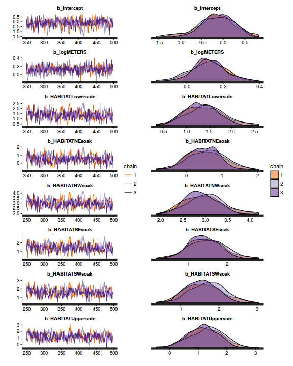
grid.arrange(stan_trace(moths.brmNB$fit, ncol=1), stan_dens(moths.brmNB$fit, separate_chains=TRUE,ncol=1), ncol=2)
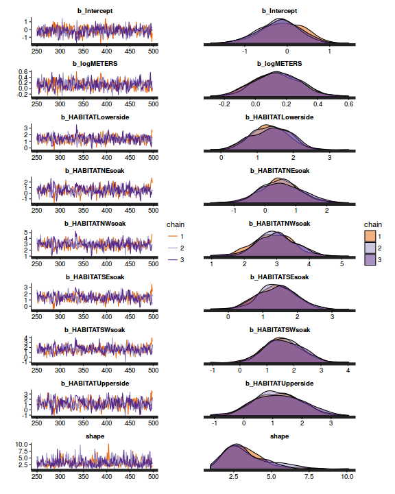
grid.arrange(stan_trace(moths.brmPO$fit, ncol=1), stan_dens(moths.brmPO$fit, separate_chains=TRUE,ncol=1), ncol=2)
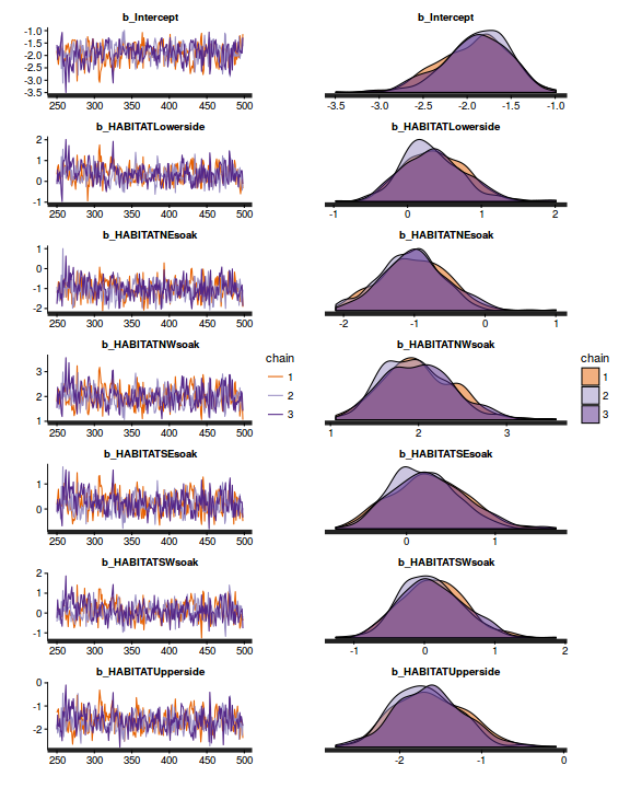
grid.arrange(stan_trace(moths.brmNBO$fit, ncol=1), stan_dens(moths.brmNBO$fit, separate_chains=TRUE,ncol=1), ncol=2)
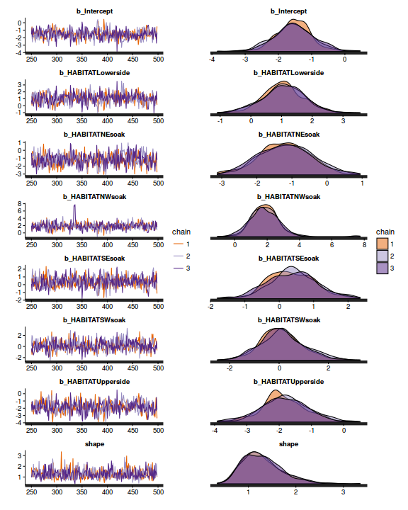
- Autocorrelation
Show code
stan_ac(moths.brmP$fit)
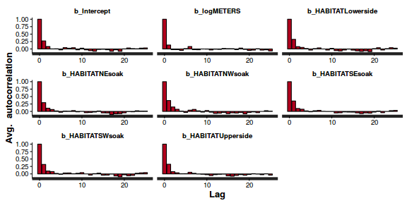
stan_ac(moths.brmNB$fit)
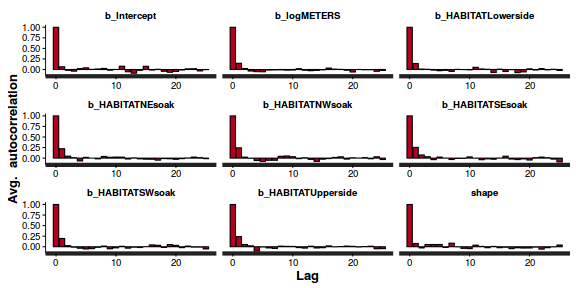
stan_ac(moths.brmPO$fit)
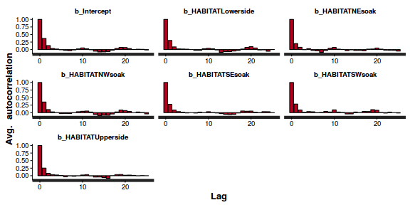
stan_ac(moths.brmNBO$fit)
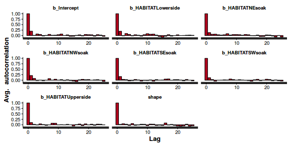
- Step size characteristics (STAN only)
Show code
summary(do.call(rbind, args = get_sampler_params(moths.brmP$fit, inc_warmup = FALSE)), digits = 2)
accept_stat__ stepsize__ treedepth__ n_leapfrog__ n_divergent__ Min. :0.39 Min. :0.26 Min. :2.0 Min. : 3 Min. :0 1st Qu.:0.86 1st Qu.:0.26 1st Qu.:3.0 1st Qu.: 7 1st Qu.:0 Median :0.94 Median :0.26 Median :3.0 Median : 7 Median :0 Mean :0.90 Mean :0.27 Mean :3.3 Mean :10 Mean :0 3rd Qu.:0.98 3rd Qu.:0.30 3rd Qu.:4.0 3rd Qu.:15 3rd Qu.:0 Max. :1.00 Max. :0.30 Max. :5.0 Max. :31 Max. :0
stan_diag(moths.brmP$fit)
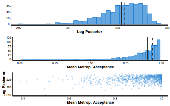
stan_diag(moths.brmP$fit, information = "stepsize")
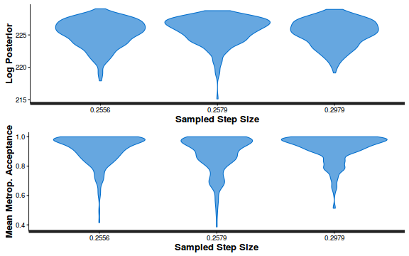
stan_diag(moths.brmP$fit, information = "treedepth")
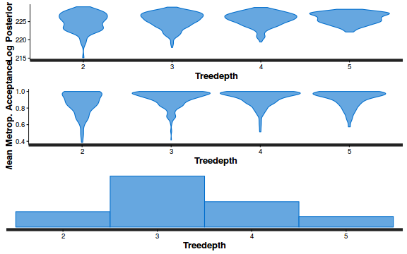
stan_diag(moths.brmP$fit, information = "divergence")
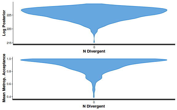
library(gridExtra) grid.arrange(stan_rhat(moths.brmP$fit) + theme_classic(8), stan_ess(moths.brmP$fit) + theme_classic(8), stan_mcse(moths.brmP$fit) + theme_classic(8), ncol = 2)
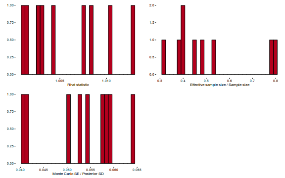
summary(do.call(rbind, args = get_sampler_params(moths.brmNB$fit, inc_warmup = FALSE)), digits = 2)
accept_stat__ stepsize__ treedepth__ n_leapfrog__ n_divergent__ Min. :0.43 Min. :0.33 Min. :2.0 Min. : 3.0 Min. :0 1st Qu.:0.86 1st Qu.:0.33 1st Qu.:3.0 1st Qu.: 7.0 1st Qu.:0 Median :0.94 Median :0.34 Median :3.0 Median : 7.0 Median :0 Mean :0.90 Mean :0.34 Mean :3.1 Mean : 8.5 Mean :0 3rd Qu.:0.98 3rd Qu.:0.36 3rd Qu.:3.0 3rd Qu.: 7.0 3rd Qu.:0 Max. :1.00 Max. :0.36 Max. :5.0 Max. :31.0 Max. :0
stan_diag(moths.brmNB$fit)
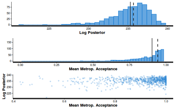
stan_diag(moths.brmNB$fit, information = "stepsize")
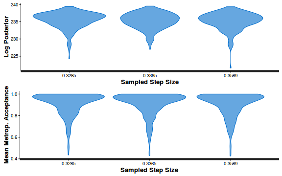
stan_diag(moths.brmNB$fit, information = "treedepth")
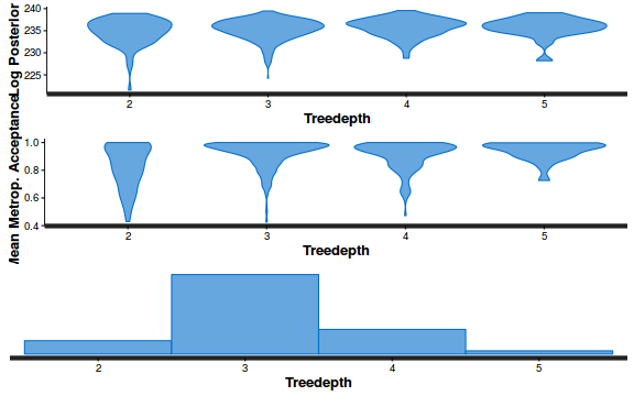
stan_diag(moths.brmNB$fit, information = "divergence")
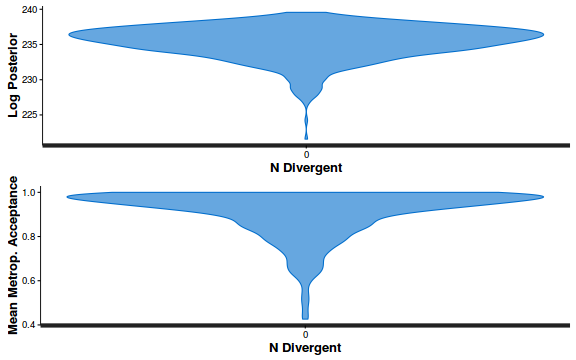
library(gridExtra) grid.arrange(stan_rhat(moths.brmNB$fit) + theme_classic(8), stan_ess(moths.brmNB$fit) + theme_classic(8), stan_mcse(moths.brmNB$fit) + theme_classic(8), ncol = 2)
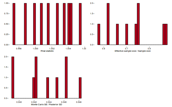
summary(do.call(rbind, args = get_sampler_params(moths.brmPO$fit, inc_warmup = FALSE)), digits = 2)
accept_stat__ stepsize__ treedepth__ n_leapfrog__ n_divergent__ Min. :0.36 Min. :0.28 Min. :1 Min. : 1.0 Min. :0 1st Qu.:0.85 1st Qu.:0.28 1st Qu.:2 1st Qu.: 3.0 1st Qu.:0 Median :0.94 Median :0.31 Median :3 Median : 7.0 Median :0 Mean :0.90 Mean :0.31 Mean :3 Mean : 7.6 Mean :0 3rd Qu.:0.98 3rd Qu.:0.32 3rd Qu.:3 3rd Qu.: 7.0 3rd Qu.:0 Max. :1.00 Max. :0.32 Max. :5 Max. :31.0 Max. :0
stan_diag(moths.brmPO$fit)
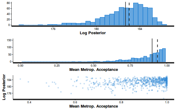
stan_diag(moths.brmPO$fit, information = "stepsize")
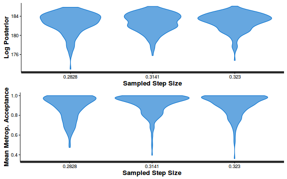
stan_diag(moths.brmPO$fit, information = "treedepth")
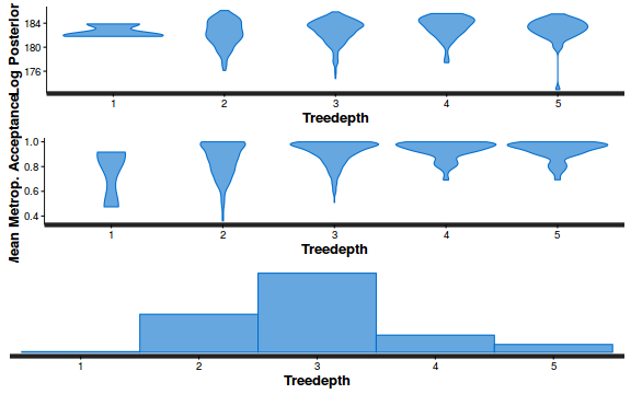
stan_diag(moths.brmPO$fit, information = "divergence")
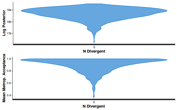
library(gridExtra) grid.arrange(stan_rhat(moths.brmPO$fit) + theme_classic(8), stan_ess(moths.brmPO$fit) + theme_classic(8), stan_mcse(moths.brmPO$fit) + theme_classic(8), ncol = 2)
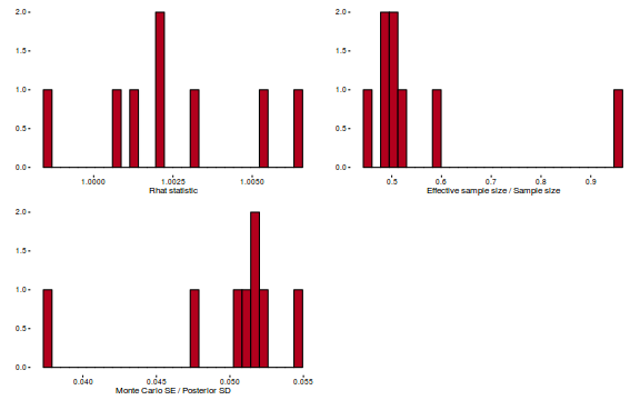
summary(do.call(rbind, args = get_sampler_params(moths.brmNBO$fit, inc_warmup = FALSE)), digits = 2)
accept_stat__ stepsize__ treedepth__ n_leapfrog__ n_divergent__ Min. :0.39 Min. :0.41 Min. :1.0 Min. : 1.0 Min. :0 1st Qu.:0.88 1st Qu.:0.41 1st Qu.:3.0 1st Qu.: 7.0 1st Qu.:0 Median :0.96 Median :0.44 Median :3.0 Median : 7.0 Median :0 Mean :0.91 Mean :0.43 Mean :2.8 Mean : 6.6 Mean :0 3rd Qu.:0.99 3rd Qu.:0.44 3rd Qu.:3.0 3rd Qu.: 7.0 3rd Qu.:0 Max. :1.00 Max. :0.44 Max. :4.0 Max. :15.0 Max. :0
stan_diag(moths.brmNBO$fit)
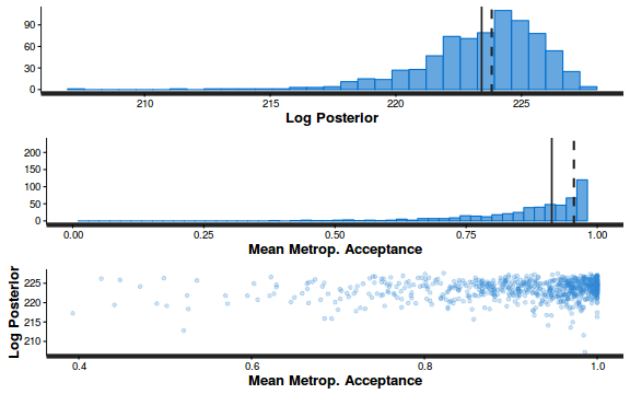
stan_diag(moths.brmNBO$fit, information = "stepsize")
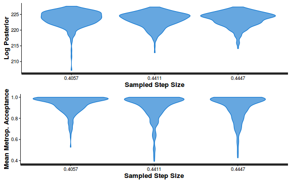
stan_diag(moths.brmNBO$fit, information = "treedepth")
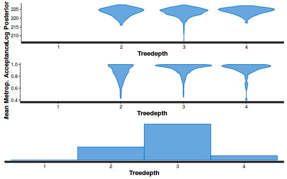
stan_diag(moths.brmNBO$fit, information = "divergence")
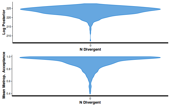
library(gridExtra) grid.arrange(stan_rhat(moths.brmNBO$fit) + theme_classic(8), stan_ess(moths.brmNBO$fit) + theme_classic(8), stan_mcse(moths.brmNBO$fit) + theme_classic(8), ncol = 2)
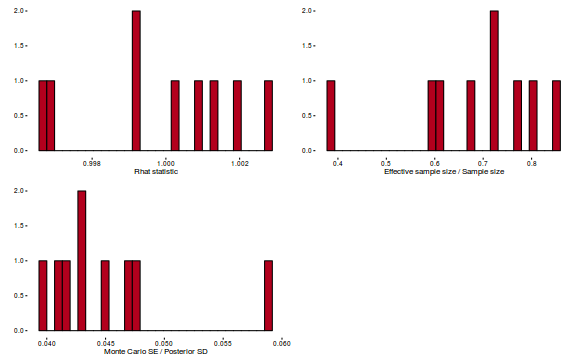
- Trace plots
- Explore the model fit diagnostics.
- Explore the patterns in simulated residuals:
Show code
simRes <- function(lambda, Y,n=250, plot=T, family='negbin', size=NULL,theta=NULL) { require(gap) N = length(Y) sim = switch(family, 'poisson' = matrix(rpois(n*N,apply(lambda,2,mean)),ncol=N, byrow=TRUE), 'negbin' = matrix(MASS:::rnegbin(n*N,apply(lambda,2,mean),mean(size)),ncol=N, byrow=TRUE), 'zip' = matrix(gamlss.dist:::rZIP(n*N,apply(lambda,2,mean),theta),ncol=N, byrow=TRUE), 'zinb' = matrix(gamlss.dist:::rZINBI(n*N,apply(lambda,2,mean),sigma=theta,nu=mean(size)),ncol=N, byrow=TRUE) ) a = apply(sim + runif(n,-0.5,0.5),2,ecdf) resid<-NULL for (i in 1:length(Y)) resid<-c(resid,a[[i]](Y[i] + runif(1 ,-0.5,0.5))) if (plot==T) { par(mfrow=c(1,2)) gap::qqunif(resid,pch = 2, bty = "n", logscale = F, col = "black", cex = 0.6, main = "QQ plot residuals", cex.main = 1, las=1) plot(resid~apply(lambda,2,mean), xlab='Predicted value', ylab='Standardized residual', las=1) } resid } lambda.brm = fitted(moths.brmP, scale='response', summary=FALSE) simRes(lambda.brm, moths$A, family='poisson')
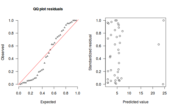
[1] 0.000 0.092 0.756 0.008 0.952 0.952 0.024 0.076 0.024 1.000 0.648 1.000 0.740 0.140 0.024 0.540 0.424 0.716 0.624 0.832 0.624 0.848 0.100 0.332 0.440 0.964 0.232 0.772 0.192 0.060 0.064 0.488 0.220 0.928 1.000 0.056 0.204 0.976 0.052 0.888
lambda.brm = fitted(moths.brmNB, scale='response', summary=FALSE) size = rstan:::extract(moths.brmNB$fit, 'shape')[[1]] simRes(lambda.brm, moths$A, family='negbin', size=size)
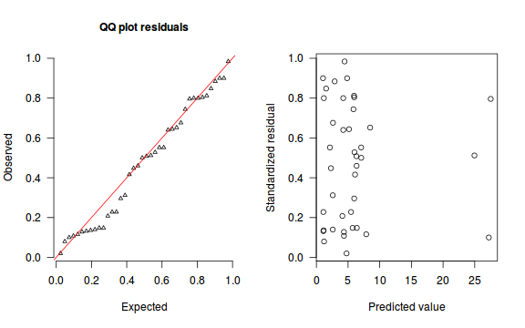
[1] 0.100 0.116 0.500 0.020 0.744 0.848 0.136 0.228 0.132 0.796 0.552 0.984 0.644 0.208 0.108 0.528 0.552 0.800 0.512 0.652 0.640 0.800 0.148 0.460 0.448 0.900 0.416 0.676 0.228 0.128 0.296 0.508 0.312 0.812 0.900 0.148 0.080 0.884 0.140 0.804
lambda.brm = fitted(moths.brmPO, scale='response', summary=FALSE) simRes(lambda.brm, moths$A, family='poisson')
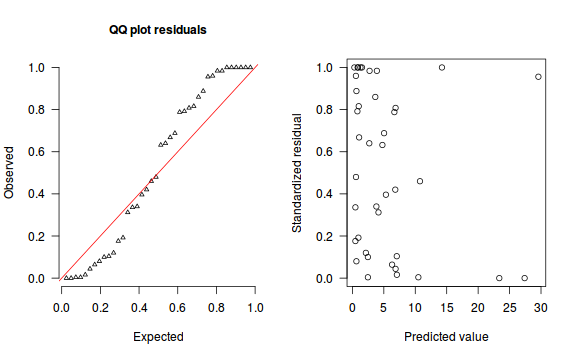
[1] 0.000 0.064 0.000 0.120 0.984 0.312 0.080 0.176 0.336 0.956 0.984 1.000 0.860 0.888 0.668 0.632 0.960 0.792 1.000 0.460 1.000 1.000 0.016 0.104 0.816 1.000 0.396 0.640 0.340 0.480 0.044 0.420 0.100 0.788 1.000 0.004 0.192 0.688 0.004 0.808
lambda.brm = fitted(moths.brmNBO, scale='response', summary=FALSE) size = rstan:::extract(moths.brmNB$fit, 'shape')[[1]] simRes(lambda.brm, moths$A, family='negbin', size=size)
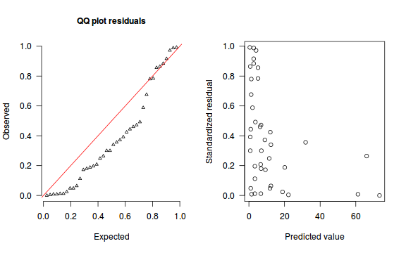
[1] 0.008 0.048 0.000 0.012 0.856 0.208 0.048 0.392 0.300 0.264 0.784 0.972 0.248 0.588 0.112 0.460 0.864 0.676 0.356 0.188 0.884 0.916 0.004 0.172 0.780 0.992 0.300 0.492 0.180 0.444 0.064 0.372 0.196 0.424 0.988 0.024 0.008 0.472 0.012 0.340
- Goodness of fit test:
Show code
## Poisson Resid.brm <- residuals(moths.brmP, type='pearson', summary=FALSE) SSres.brm <- apply(Resid.brm^2,1,sum) lambda.brm = fitted(moths.brm, scale='response', summary=FALSE) YNew.brm <- matrix(rpois(length(lambda.brm), lambda=lambda.brm),nrow=nrow(lambda.brm)) Resid1.brm<-(lambda.brm - YNew.brm)/sqrt(lambda.brm) SSres.sim.brm<-apply(Resid1.brm^2,1,sum) mean(SSres.sim.brm>SSres.brm)
[1] 0.005333333
## Negative Binomial Resid.brm <- residuals(moths.brmNB, type='pearson', summary=FALSE) SSres.brm <- apply(Resid.brm^2,1,sum) lambda.brm = fitted(moths.brm, scale='response', summary=FALSE) YNew.brm <- matrix(rpois(length(lambda.brm), lambda=lambda.brm),nrow=nrow(lambda.brm)) Resid1.brm<-(lambda.brm - YNew.brm)/sqrt(lambda.brm) SSres.sim.brm<-apply(Resid1.brm^2,1,sum) mean(SSres.sim.brm>SSres.brm)
[1] 0.8346667
## Poisson with offset Resid.brm <- residuals(moths.brmPO, type='pearson', summary=FALSE) SSres.brm <- apply(Resid.brm^2,1,sum) lambda.brm = fitted(moths.brm, scale='response', summary=FALSE) YNew.brm <- matrix(rpois(length(lambda.brm), lambda=lambda.brm),nrow=nrow(lambda.brm)) Resid1.brm<-(lambda.brm - YNew.brm)/sqrt(lambda.brm) SSres.sim.brm<-apply(Resid1.brm^2,1,sum) mean(SSres.sim.brm>SSres.brm)
[1] 0
## Negative Binomial with offset Resid.brm <- residuals(moths.brmNBO, type='pearson', summary=FALSE) SSres.brm <- apply(Resid.brm^2,1,sum) lambda.brm = fitted(moths.brm, scale='response', summary=FALSE) YNew.brm <- matrix(rpois(length(lambda.brm), lambda=lambda.brm),nrow=nrow(lambda.brm)) Resid1.brm<-(lambda.brm - YNew.brm)/sqrt(lambda.brm) SSres.sim.brm<-apply(Resid1.brm^2,1,sum) mean(SSres.sim.brm>SSres.brm)
[1] 0.872
- Fitted and observed values (plot):
Show code
## Poisson newdata <- data.frame(HABITAT=levels(moths$HABITAT), METERS=mean(moths$METERS)) tempdata = fitted(moths.brmP, scale='response',newdata=newdata) tempdata <- cbind(newdata, Mean=tempdata[,'Estimate'], Lower=tempdata[,'2.5%ile'], Upper=tempdata[,'97.5%ile']) tempdata
HABITAT METERS Mean Lower Upper 1 Disturbed 45.5 1.474522 0.5637094 3.031730 2 Lowerside 45.5 5.457930 3.5429458 7.981774 3 NEsoak 45.5 2.377828 1.2604467 3.745447 4 NWsoak 45.5 26.209140 19.6452112 34.361091 5 SEsoak 45.5 5.851585 4.0600126 8.137415 6 SWsoak 45.5 6.959453 4.2331902 10.367149 7 Upperside 45.5 4.761405 2.9405168 6.993508
library(ggplot2) ggplot(moths, aes(y=A, x=HABITAT)) + geom_boxplot() + geom_pointrange(data=tempdata,aes(y=Mean, ymin=Lower, ymax=Upper), color='red')

##OR the manual way Xmat <- model.matrix(~log(METERS) + HABITAT, data=newdata) coefs <- as.matrix(as.data.frame(rstan:::extract(moths.brmP$fit))) coefs <- coefs[,grep('^b_', colnames(coefs))] fit = exp(coefs %*% t(Xmat)) tempdata <- cbind(newdata, plyr:::adply(fit, 2, function(x) { data.frame(Mean=mean(x), Median=median(x), HPDinterval(as.mcmc(x))) })) ggplot(moths, aes(y=A, x=HABITAT)) + geom_boxplot() + geom_pointrange(data=tempdata,aes(y=Mean, ymin=lower, ymax=upper), color='red')
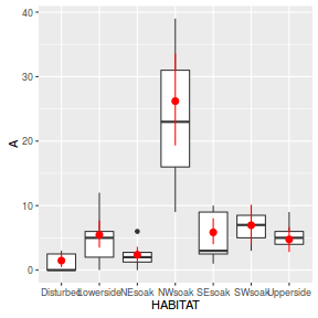
## Negative Binomial newdata <- data.frame(HABITAT=levels(moths$HABITAT), METERS=mean(moths$METERS)) tempdata = fitted(moths.brmNB, scale='response',newdata=newdata) tempdata <- cbind(newdata, Mean=tempdata[,'Estimate'], Lower=tempdata[,'2.5%ile'], Upper=tempdata[,'97.5%ile']) library(ggplot2) ggplot(moths, aes(y=A, x=HABITAT)) + geom_boxplot() + geom_pointrange(data=tempdata,aes(y=Mean, ymin=Lower, ymax=Upper), color='red')
##OR the manual way Xmat <- model.matrix(~log(METERS) + HABITAT, data=newdata) coefs <- as.matrix(as.data.frame(rstan:::extract(moths.brmNB$fit))) coefs <- coefs[,grep('^b_', colnames(coefs))] fit = exp(coefs %*% t(Xmat)) tempdata <- cbind(newdata, plyr:::adply(fit, 2, function(x) { data.frame(Mean=mean(x), Median=median(x), HPDinterval(as.mcmc(x))) })) ggplot(moths, aes(y=A, x=HABITAT)) + geom_boxplot() + geom_pointrange(data=tempdata,aes(y=Mean, ymin=lower, ymax=upper), color='red')
## Poisson with offset newdata <- data.frame(HABITAT=levels(moths$HABITAT), METERS=mean(moths$METERS)) tempdata = fitted(moths.brmPO, scale='response',newdata=newdata) tempdata <- cbind(newdata, Mean=tempdata[,'Estimate'], Lower=tempdata[,'2.5%ile'], Upper=tempdata[,'97.5%ile']) library(ggplot2) ggplot(moths, aes(y=A, x=HABITAT)) + geom_boxplot() + geom_pointrange(data=tempdata,aes(y=Mean, ymin=Lower, ymax=Upper), color='red')
##OR the manual way - dont forget to account for the offset Xmat <- model.matrix(~HABITAT, data=newdata) coefs <- as.matrix(as.data.frame(rstan:::extract(moths.brmPO$fit))) coefs <- coefs[,grep('^b_', colnames(coefs))] fit = exp(coefs %*% t(Xmat) + log(mean(moths$METERS))) tempdata <- cbind(newdata, plyr:::adply(fit, 2, function(x) { data.frame(Mean=mean(x), Median=median(x), HPDinterval(as.mcmc(x))) })) ggplot(moths, aes(y=A, x=HABITAT)) + geom_boxplot() + geom_pointrange(data=tempdata,aes(y=Mean, ymin=lower, ymax=upper), color='red')
## Negative Binomial with offset newdata <- data.frame(HABITAT=levels(moths$HABITAT), METERS=mean(moths$METERS)) tempdata = fitted(moths.brmNBO, scale='response',newdata=newdata) tempdata <- cbind(newdata, Mean=tempdata[,'Estimate'], Lower=tempdata[,'2.5%ile'], Upper=tempdata[,'97.5%ile']) library(ggplot2) ggplot(moths, aes(y=A, x=HABITAT)) + geom_boxplot() + geom_pointrange(data=tempdata,aes(y=Mean, ymin=Lower, ymax=Upper), color='red')
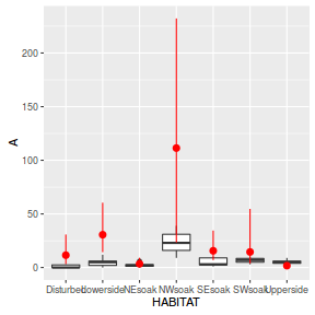
##OR the manual way Xmat <- model.matrix(~HABITAT, data=newdata) coefs <- as.matrix(as.data.frame(rstan:::extract(moths.brmNBO$fit))) coefs <- coefs[,grep('^b_', colnames(coefs))] fit = exp(coefs %*% t(Xmat) + log(mean(moths$METERS))) tempdata <- cbind(newdata, plyr:::adply(fit, 2, function(x) { data.frame(Mean=mean(x), Median=median(x), HPDinterval(as.mcmc(x))) })) ggplot(moths, aes(y=A, x=HABITAT)) + geom_boxplot() + geom_pointrange(data=tempdata,aes(y=Mean, ymin=lower, ymax=upper), color='red')
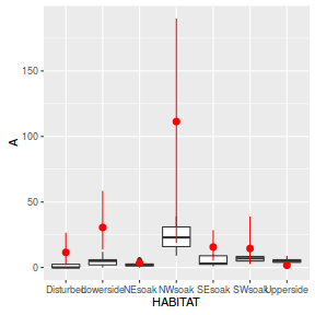
- Check for overdispersion:
Show code
## Poisson coefs <- as.matrix(as.data.frame(rstan:::extract(moths.brmP$fit))) coefs <- coefs[,grep('^b_', colnames(coefs))] Resid <- residuals(moths.brmP, type='pearson',summary=FALSE) RSS <- apply(Resid^2,1,sum) Disp <- RSS/(nrow(moths)-ncol(coefs)) data.frame(Median=median(Disp), Mean=mean(Disp), HPDinterval(as.mcmc(Disp)))
Median Mean lower upper var1 2.42229 2.442048 2.273809 2.671013
## Negative Binomial coefs <- as.matrix(as.data.frame(rstan:::extract(moths.brmNB$fit))) coefs <- coefs[,grep('^b_', colnames(coefs))] Resid <- residuals(moths.brmNB, type='pearson',summary=FALSE) RSS <- apply(Resid^2,1,sum) Disp <- RSS/(nrow(moths)-ncol(coefs)) data.frame(Median=median(Disp), Mean=mean(Disp), HPDinterval(as.mcmc(Disp)))
Median Mean lower upper var1 0.8497883 0.9132843 0.7213029 1.304696
## Poisson with offset coefs <- as.matrix(as.data.frame(rstan:::extract(moths.brmPO$fit))) coefs <- coefs[,grep('^b_', colnames(coefs))] Resid <- residuals(moths.brmPO, type='pearson',summary=FALSE) RSS <- apply(Resid^2,1,sum) Disp <- RSS/(nrow(moths)-ncol(coefs)) data.frame(Median=median(Disp), Mean=mean(Disp), HPDinterval(as.mcmc(Disp)))
Median Mean lower upper var1 8.512843 8.533245 8.35746 8.765346
## Negative Binomial with offset coefs <- as.matrix(as.data.frame(rstan:::extract(moths.brmNBO$fit))) coefs <- coefs[,grep('^b_', colnames(coefs))] Resid <- residuals(moths.brmNBO, type='pearson',summary=FALSE) RSS <- apply(Resid^2,1,sum) Disp <- RSS/(nrow(moths)-ncol(coefs)) data.frame(Median=median(Disp), Mean=mean(Disp), HPDinterval(as.mcmc(Disp)))
Median Mean lower upper var1 0.7153655 0.9899389 0.6280123 1.46994
- Explore the patterns in simulated residuals:
- At this stage we will conclude that the offset models are poor fits.
The Negative Binomial model appears to be a better fit than the Poisson, the latter of which
is overdispersed.
Explore the parameter estimates for the Negative Binomial model.
Show code
summary(moths.brmNB)
Family: negbinomial (log) Formula: A ~ log(METERS) + HABITAT Data: moths (Number of observations: 40) Samples: 3 chains, each with iter = 2000; warmup = 1000; thin = 4; total post-warmup samples = 750 WAIC: Not computed Fixed Effects: Estimate Est.Error l-95% CI u-95% CI Eff.Sample Rhat Intercept -0.16 0.50 -1.17 0.76 651 1.01 logMETERS 0.14 0.15 -0.14 0.42 566 1.00 HABITATLowerside 1.37 0.52 0.38 2.32 556 1.00 HABITATNEsoak 0.51 0.66 -0.75 1.85 492 1.00 HABITATNWsoak 2.95 0.61 1.79 4.17 466 1.00 HABITATSEsoak 1.40 0.55 0.36 2.50 431 1.00 HABITATSWsoak 1.62 0.69 0.37 2.98 523 1.00 HABITATUpperside 1.18 0.81 -0.27 2.75 464 1.00 Family Specific Parameters: Estimate Est.Error l-95% CI u-95% CI Eff.Sample Rhat shape 3.27 1.41 1.31 6.8 649 1 Samples were drawn using sampling(NUTS). For each parameter, Eff.Sample is a crude measure of effective sample size, and Rhat is the potential scale reduction factor on split chains (at convergence, Rhat = 1).exp(coef(moths.brmNB))
mean Intercept 0.8530651 logMETERS 1.1495789 HABITATLowerside 3.9311608 HABITATNEsoak 1.6688071 HABITATNWsoak 19.0893054 HABITATSEsoak 4.0741209 HABITATSWsoak 5.0406178 HABITATUpperside 3.2528957
coefs.brm <- as.matrix(as.data.frame(rstan:::extract(moths.brmNB$fit))) coefs.brm <- coefs.brm[,grep('b', colnames(coefs.brm))] plyr:::adply(exp(coefs.brm), 2, function(x) { data.frame(Mean=mean(x), median=median(x), HPDinterval(as.mcmc(x))) })
X1 Mean median lower upper 1 b_Intercept 0.9640476 0.8667087 0.2455259 1.924904 2 b_logMETERS 1.1622245 1.1454692 0.8537851 1.493643 3 b_HABITATLowerside 4.4979287 4.0014549 1.0605590 8.794885 4 b_HABITATNEsoak 2.0883054 1.6512687 0.2406724 5.097136 5 b_HABITATNWsoak 23.0365909 19.1029295 2.6240569 52.580216 6 b_HABITATSEsoak 4.7417832 4.1066968 0.7076325 9.973949 7 b_HABITATSWsoak 6.4842791 4.9137160 0.8596906 15.789222 8 b_HABITATUpperside 4.5218465 3.1861182 0.3221937 12.337032
marginal_effects(moths.brmNB, effects='HABITAT')
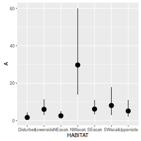
- Estimate the strength of the relationship
Show code
## calculate the expected values on the response scale lambda.brm = fitted(moths.brmNB, scale='response', summary=FALSE) ## calculate the raw SSresid SSres.brm <- apply((-1*(sweep(lambda.brm,2, moths$A,'-')))^2,1,sum) SSres.null <- sum((moths$A - mean(moths$A))^2) #OR #calculate the model r2 1-mean(SSres.brm)/SSres.null
[1] 0.3798634
#OR manually coefs <- as.matrix(as.data.frame(rstan:::extract(moths.brmNB$fit))) coefs <- coefs[,grep('^b_', colnames(coefs))] Xmat <- model.matrix(~log(METERS) + HABITAT, data=moths) lambda.brm = exp(coefs %*% t(Xmat)) ## calculate the raw SSresid SSres.brm <- apply((-1*(sweep(lambda.brm,2,moths$A,'-')))^2,1,sum) SSres.null <- crossprod(moths$A - mean(moths$A)) #calculate the model r2 1-mean(SSres.brm)/SSres.null
[,1] [1,] 0.3798634
## Alternatively.. R.var = apply(residuals(moths.brmNB, summary=FALSE),1,var) X.var = apply(fitted(moths.brmNB, summary=FALSE),1,var) R2.marginal <- X.var/(X.var + R.var) data.frame(Median=median(R2.marginal), coda:::HPDinterval(as.mcmc(R2.marginal)))
Median lower upper var1 0.6292283 0.3216714 0.7238538
- Although we have now established that there is a statistical difference between the group means,
we do not yet know which group(s) are different from which other(s).
To address this we can explore all pairwise contrasts from the posterior. Note, careful when back transforming from log.
Recall that log laws indicate that $log(a) - log(b) = log(a/b)$.
Show code
coefs <-as.matrix(as.data.frame(rstan:::extract(moths.brmNB$fit))) coefs <- coefs[,grep('^b_', colnames(coefs))] newdata <- data.frame(HABITAT=levels(moths$HABITAT), METERS=mean(moths$METERS)) Xmat <- model.matrix(~log(METERS) + HABITAT, data=newdata) library(multcomp) tuk.mat <- contrMat(n=table(newdata$HABITAT), type="Tukey") Xmat <- model.matrix(~log(METERS)+HABITAT, data=newdata) Xmat <- tuk.mat %*% Xmat fit <- exp(coefs %*% t(Xmat)) library(coda) MCMCsum <- function(x) { data.frame(Median=median(x, na.rm=TRUE), t(quantile(x,na.rm=TRUE)), HPDinterval(as.mcmc(x))) } plyr:::adply(as.matrix(fit),2,MCMCsum)
X1 Median X0. X25. X50. X75. X100. lower upper 1 Lowerside - Disturbed 4.0014549 0.75058230 2.6927014 4.0014549 5.7029870 34.0094273 1.06055902 8.7948850 2 NEsoak - Disturbed 1.6512687 0.17191247 1.0657961 1.6512687 2.5321403 15.0458543 0.24067244 5.0971364 3 NWsoak - Disturbed 19.1029295 2.62405689 12.8337712 19.1029295 27.8190728 183.3046958 2.62405689 52.5802164 4 SEsoak - Disturbed 4.1066968 0.59830817 2.8466216 4.1066968 5.7985525 32.5714541 0.70763248 9.9739487 5 SWsoak - Disturbed 4.9137160 0.33815372 3.1774973 4.9137160 8.0255117 55.9231149 0.85969057 15.7892225 6 Upperside - Disturbed 3.1861182 0.32219367 1.8454384 3.1861182 5.6032516 36.7013276 0.32219367 12.3370325 7 NEsoak - Lowerside 0.4302645 0.09341336 0.3011472 0.4302645 0.5996800 1.7768091 0.12722450 0.9474301 8 NWsoak - Lowerside 4.7596871 1.40687834 3.5717100 4.7596871 6.6442824 22.2970521 1.40687834 10.2087762 9 SEsoak - Lowerside 1.0230626 0.30087781 0.8127477 1.0230626 1.3137698 3.8331690 0.49229150 2.0169133 10 SWsoak - Lowerside 1.2891018 0.16286740 0.8997906 1.2891018 1.8098058 7.7462736 0.16286740 3.0991319 11 Upperside - Lowerside 0.8160707 0.15518045 0.5505156 0.8160707 1.2557586 5.5328028 0.15518045 2.2845561 12 NWsoak - NEsoak 11.3275794 2.38413610 7.9713011 11.3275794 16.4057151 74.0606945 3.52147567 27.5885849 13 SEsoak - NEsoak 2.4364756 0.49206697 1.7481048 2.4364756 3.4164552 8.6936643 0.70461238 5.4812849 14 SWsoak - NEsoak 2.9909563 0.49728521 2.0435734 2.9909563 4.3208633 22.0843886 0.64089541 7.6826544 15 Upperside - NEsoak 1.9914847 0.17379858 1.4008755 1.9914847 2.7697335 13.3831349 0.39992138 4.8920306 16 SEsoak - NWsoak 0.2155425 0.05343626 0.1554463 0.2155425 0.2892431 0.9090968 0.08251825 0.4751569 17 SWsoak - NWsoak 0.2691229 0.04348677 0.1833171 0.2691229 0.3791270 1.4805610 0.06255997 0.6595744 18 Upperside - NWsoak 0.1718971 0.02995233 0.1149770 0.1718971 0.2468979 0.9966972 0.02995233 0.4584054 19 SWsoak - SEsoak 1.2630026 0.14038551 0.8964932 1.2630026 1.7209516 8.8383401 0.27528176 2.8265154 20 Upperside - SEsoak 0.7956164 0.13375965 0.5553199 0.7956164 1.1470159 5.5829958 0.13375965 2.0120800 21 Upperside - SWsoak 0.6492371 0.10376765 0.4309988 0.6492371 0.9598559 5.3098336 0.11219507 1.7852750
## Due to log laws, these effects are multipliers rather than differences ## If you want to express the outcomes in terms of differences then it is necessary to ## estimate the cell posteriors and subtract those - this cannot easily be done Frequentist! Xmat <- model.matrix(~log(METERS) + HABITAT, data=newdata) fit <- exp(coefs %*% t(Xmat)) library(multcomp) tuk.mat <- contrMat(n=table(newdata$HABITAT), type="Tukey") fit <- fit %*% t(tuk.mat) plyr:::adply(as.matrix(fit),2,MCMCsum)
X1 Median X0. X25. X50. X75. X100. lower upper 1 Lowerside - Disturbed 4.0689569 -2.202499 3.0265807 4.0689569 5.3089091 14.57838684 1.2409552 8.1448004 2 NEsoak - Disturbed 0.9017660 -7.312479 0.1340833 0.9017660 1.6467105 6.94889870 -1.8583399 3.6882766 3 NWsoak - Disturbed 25.4062806 9.963564 20.2980553 25.4062806 32.7550632 85.26925867 10.6408161 51.6049801 4 SEsoak - Disturbed 4.2722895 -2.581770 3.3043011 4.2722895 5.4839030 14.10709025 1.0868378 8.2307350 5 SWsoak - Disturbed 5.7266432 -3.546058 3.8621775 5.7266432 8.1649238 31.40750951 0.2218100 13.8002744 6 Upperside - Disturbed 3.0285388 -5.831655 1.6724786 3.0285388 4.9985728 16.28502930 -0.8236566 9.9717337 7 NEsoak - Lowerside -3.1348894 -14.535877 -4.6852567 -3.1348894 -1.9589919 3.03830738 -8.6001836 0.6197858 8 NWsoak - Lowerside 21.3923404 3.912020 15.6498096 21.3923404 28.6200122 78.99186890 4.2933904 46.4128749 9 SEsoak - Lowerside 0.1404985 -10.703890 -1.1670427 0.1404985 1.5726694 11.06519437 -5.7490841 4.1488093 10 SWsoak - Lowerside 1.7227120 -10.186649 -0.5544462 1.7227120 3.9412710 27.85100117 -5.1579731 12.1380466 11 Upperside - Lowerside -1.0124225 -12.908841 -3.0498762 -1.0124225 1.2095389 12.87205248 -7.8457054 6.6083564 12 NWsoak - NEsoak 24.7864257 7.193430 19.1047828 24.7864257 32.1681075 85.29390321 7.1934299 50.4455294 13 SEsoak - NEsoak 3.3941761 -3.446630 2.1103394 3.3941761 4.7262440 12.75358000 -0.2609212 8.8197256 14 SWsoak - NEsoak 4.6908240 -2.163572 2.9268259 4.6908240 7.1472431 30.53130201 -0.3405123 14.5425090 15 Upperside - NEsoak 2.3346951 -9.374825 1.0356404 2.3346951 3.7770028 15.27627974 -2.4397183 7.7411171 16 SEsoak - NWsoak -20.9607257 -77.798077 -28.8479819 -20.9607257 -15.6463026 -1.08124784 -47.7083030 -6.1904502 17 SWsoak - NWsoak -19.5044667 -81.107760 -26.6646773 -19.5044667 -13.4849094 9.43627683 -47.2339163 -0.3334677 18 Upperside - NWsoak -22.5288701 -82.524769 -29.9152465 -22.5288701 -16.3370635 -0.03711989 -50.4070421 -4.8827190 19 SWsoak - SEsoak 1.5127864 -11.093903 -0.7095885 1.5127864 3.9371915 28.36110107 -5.4554441 10.4675256 20 Upperside - SEsoak -1.1427166 -12.535355 -3.0425532 -1.1427166 0.7945388 14.15899246 -6.9809698 6.0547850 21 Upperside - SWsoak -2.3541702 -23.471257 -5.2799897 -2.3541702 -0.2025978 12.69251435 -12.3680295 5.9271043
- Produce a suitable summary plot
Show code
coefs <-as.matrix(as.data.frame(rstan:::extract(moths.brmNB$fit))) coefs <- coefs[,grep('^b_', colnames(coefs))] newdata <- data.frame(HABITAT=levels(moths$HABITAT), METERS=mean(moths$METERS)) Xmat <- model.matrix(~log(METERS) + HABITAT, data=newdata) fit = exp(coefs %*% t(Xmat)) newdata = cbind(newdata, plyr:::adply(fit, 2, function(x) { data.frame(Mean=mean(x, na.rm=TRUE),Median=median(x, na.rm=TRUE), HPDinterval(as.mcmc(x))) })) ggplot(moths, aes(y=A, x=HABITAT)) + geom_point(color='grey') + geom_pointrange(data=newdata, aes(y=Mean, ymin=lower, ymax=upper)) + scale_y_continuous('Number of Moths') + scale_x_discrete('HABITAT') + theme_classic() + theme(axis.line.x=element_line(), axis.line.y=element_line())
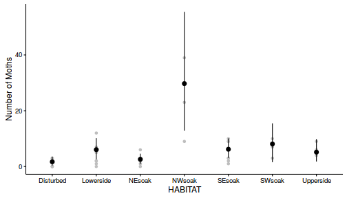
Poisson t-test with zero-inflation
Yet again our rather fixated marine ecologist has returned to the rocky shore with an interest in examining the effects of wave exposure on the abundance of yet another intertidal marine limpet Patelloida latistrigata on rocky intertidal shores. It would appear that either this ecologist is lazy, is satisfied with the methodology or else suffers from some superstition disorder (that prevents them from deviating too far from a series of tasks), and thus, yet again, a single quadrat was placed on 10 exposed (to large waves) shores and 10 sheltered shores. From each quadrat, the number of scaley limpets (Patelloida latistrigata) were counted. Initially, faculty were mildly interested in the research of this ecologist (although lets be honest, most academics usually only display interest in the work of the other members of their school out of politeness - Oh I did not say that did I?). Nevertheless, after years of attending seminars by this ecologist in which the only difference is the target species, faculty have started to display more disturbing levels of animosity towards our ecologist. In fact, only last week, the members of the school's internal ARC review panel (when presented with yet another wave exposure proposal) were rumored to take great pleasure in concocting up numerous bogus applications involving hedgehogs and balloons just so they could rank our ecologist proposal outside of the top 50 prospects and ... Actually, I may just have digressed!
Download LimpetsScaley data setFormat of limpetsScaley.csv data files Count Shore 4 sheltered 1 sheltered 2 sheltered 0 sheltered 4 sheltered ... ... Shore Categorical description of the shore type (sheltered or exposed) - Predictor variable Count Number of limpets per quadrat - Response variable 
Open the limpetsSmooth data set.
Show codelimpets <- read.table('../downloads/data/limpetsScaley.csv', header=T, sep=',', strip.white=T) limpets
Count Shore 1 2 sheltered 2 1 sheltered 3 3 sheltered 4 1 sheltered 5 0 sheltered 6 0 sheltered 7 1 sheltered 8 0 sheltered 9 2 sheltered 10 1 sheltered 11 4 exposed 12 9 exposed 13 3 exposed 14 1 exposed 15 3 exposed 16 0 exposed 17 0 exposed 18 7 exposed 19 8 exposed 20 5 exposed
-
As part of the routine exploratory data analysis:
- Explore the distribution of counts from each population
Show code
boxplot(Count~Shore,data=limpets) rug(jitter(limpets$Count), side=2)
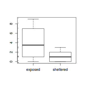
- Compare the expected number of zeros to the actual number of zeros to determine whether the model might be zero inflated.
- Calculate the proportion of zeros in the data
Show code
limpets.tab<-table(limpets$Count==0) limpets.tab/sum(limpets.tab)
FALSE TRUE 0.75 0.25
- Now work out the proportion of zeros we would expect from a Poisson distribution with a lambda equal to the mean count of limpets in this study.
Show codeClearly there are substantially more zeros than expected so the data are likely to be zero inflated.
limpets.mu <- mean(limpets$Count) cnts <-rpois(1000,limpets.mu) limpets.tab<-table(cnts==0) limpets.tab/sum(limpets.tab)
FALSE TRUE 0.91 0.09
- Calculate the proportion of zeros in the data
- Explore the distribution of counts from each population
- Lets explore a zero-inflated Poisson (ZIP) model.
$$
p(y_i|\theta,\lambda) = \left\{
\begin{array}{l l}
\theta + (1-\theta)\times \text{Pois}(0|\lambda) & \quad \text{if $y_i=0$ and}\\
(1-\theta)\times \text{Pois}(y_i|\lambda) & \quad \text{if $y_i>0$}
\end{array} \right.\\
\begin{align}
log(\lambda_i)&=\eta_i & (\text{link function})\\
\eta_i&=\beta_0+\beta_1 X_i & (\text{linear predictor})\\
\beta_0, \beta_1&\sim{}\mathcal{N}(0,1000) & (\text{week Bayesian prior})\\
\end{align}
$$
Show code
limpets.brm <- brm(Count~0+spec+main+main:Shore, family='zero_inflated_poisson', data=limpets, prior = c(set_prior("normal(0,1000)", class="b")), chains=3, iter=2000, warmup=1000, thin=4)
SAMPLING FOR MODEL 'zero_inflated_poisson(log) brms-model' NOW (CHAIN 1). Chain 1, Iteration: 1 / 2000 [ 0%] (Warmup) Chain 1, Iteration: 200 / 2000 [ 10%] (Warmup) Chain 1, Iteration: 400 / 2000 [ 20%] (Warmup) Chain 1, Iteration: 600 / 2000 [ 30%] (Warmup) Chain 1, Iteration: 800 / 2000 [ 40%] (Warmup) Chain 1, Iteration: 1000 / 2000 [ 50%] (Warmup) Chain 1, Iteration: 1001 / 2000 [ 50%] (Sampling) Chain 1, Iteration: 1200 / 2000 [ 60%] (Sampling) Chain 1, Iteration: 1400 / 2000 [ 70%] (Sampling) Chain 1, Iteration: 1600 / 2000 [ 80%] (Sampling) Chain 1, Iteration: 1800 / 2000 [ 90%] (Sampling) Chain 1, Iteration: 2000 / 2000 [100%] (Sampling)# # Elapsed Time: 0.161603 seconds (Warm-up) # 0.167162 seconds (Sampling) # 0.328765 seconds (Total) # SAMPLING FOR MODEL 'zero_inflated_poisson(log) brms-model' NOW (CHAIN 2). Chain 2, Iteration: 1 / 2000 [ 0%] (Warmup) Chain 2, Iteration: 200 / 2000 [ 10%] (Warmup) Chain 2, Iteration: 400 / 2000 [ 20%] (Warmup) Chain 2, Iteration: 600 / 2000 [ 30%] (Warmup) Chain 2, Iteration: 800 / 2000 [ 40%] (Warmup) Chain 2, Iteration: 1000 / 2000 [ 50%] (Warmup) Chain 2, Iteration: 1001 / 2000 [ 50%] (Sampling) Chain 2, Iteration: 1200 / 2000 [ 60%] (Sampling) Chain 2, Iteration: 1400 / 2000 [ 70%] (Sampling) Chain 2, Iteration: 1600 / 2000 [ 80%] (Sampling) Chain 2, Iteration: 1800 / 2000 [ 90%] (Sampling) Chain 2, Iteration: 2000 / 2000 [100%] (Sampling)# # Elapsed Time: 0.567222 seconds (Warm-up) # 0.092628 seconds (Sampling) # 0.65985 seconds (Total) # SAMPLING FOR MODEL 'zero_inflated_poisson(log) brms-model' NOW (CHAIN 3). Chain 3, Iteration: 1 / 2000 [ 0%] (Warmup) Chain 3, Iteration: 200 / 2000 [ 10%] (Warmup) Chain 3, Iteration: 400 / 2000 [ 20%] (Warmup) Chain 3, Iteration: 600 / 2000 [ 30%] (Warmup) Chain 3, Iteration: 800 / 2000 [ 40%] (Warmup) Chain 3, Iteration: 1000 / 2000 [ 50%] (Warmup) Chain 3, Iteration: 1001 / 2000 [ 50%] (Sampling) Chain 3, Iteration: 1200 / 2000 [ 60%] (Sampling) Chain 3, Iteration: 1400 / 2000 [ 70%] (Sampling) Chain 3, Iteration: 1600 / 2000 [ 80%] (Sampling) Chain 3, Iteration: 1800 / 2000 [ 90%] (Sampling) Chain 3, Iteration: 2000 / 2000 [100%] (Sampling)# # Elapsed Time: 0.35152 seconds (Warm-up) # 0.126483 seconds (Sampling) # 0.478003 seconds (Total) #
- Explore the chain mixing diagnostics.
- Trace plots
Show code
library(gridExtra) grid.arrange(stan_trace(limpets.brm$fit, ncol=1), stan_dens(limpets.brm$fit, separate_chains=TRUE,ncol=1), ncol=2)
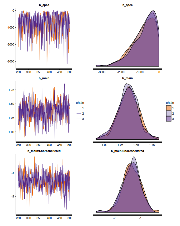
- Autocorrelation
Show code
stan_ac(limpets.brm$fit)
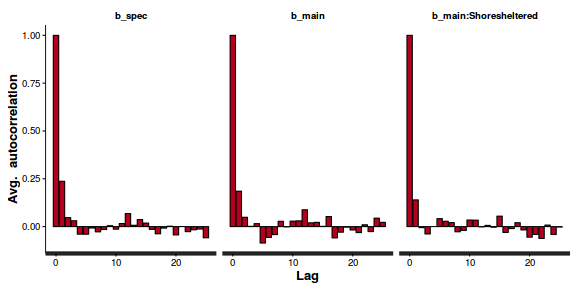
- Step size characteristics (STAN only)
Show code
summary(do.call(rbind, args = get_sampler_params(limpets.brm$fit, inc_warmup = FALSE)), digits = 2)
accept_stat__ stepsize__ treedepth__ n_leapfrog__ n_divergent__ Min. :0.00 Min. :0.22 Min. :1.0 Min. : 1.0 Min. :0.00 1st Qu.:0.80 1st Qu.:0.22 1st Qu.:3.0 1st Qu.: 4.0 1st Qu.:0.00 Median :0.93 Median :0.22 Median :3.0 Median : 7.0 Median :1.00 Mean :0.84 Mean :0.28 Mean :3.1 Mean : 7.8 Mean :0.51 3rd Qu.:1.00 3rd Qu.:0.40 3rd Qu.:4.0 3rd Qu.:11.0 3rd Qu.:1.00 Max. :1.00 Max. :0.40 Max. :5.0 Max. :24.0 Max. :1.00
stan_diag(limpets.brm$fit)
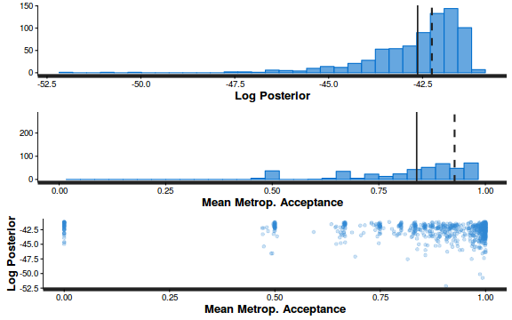
stan_diag(limpets.brm$fit, information = "stepsize")
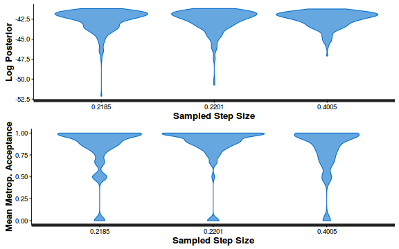
stan_diag(limpets.brm$fit, information = "treedepth")
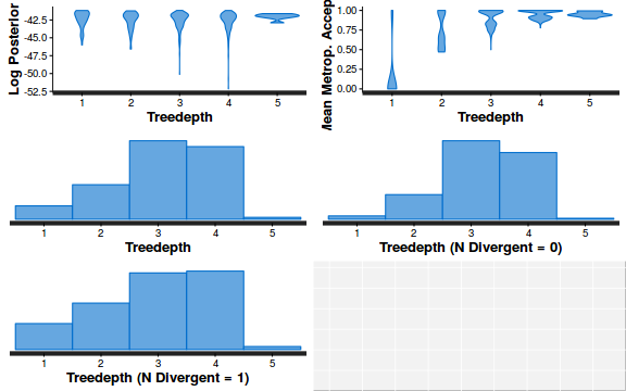
stan_diag(limpets.brm$fit, information = "divergence")
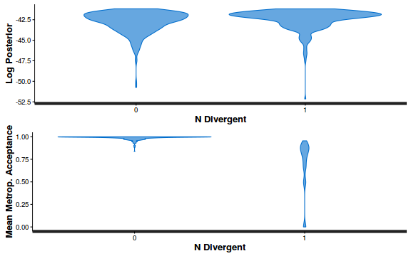
library(gridExtra) grid.arrange(stan_rhat(limpets.brm$fit) + theme_classic(8), stan_ess(limpets.brm$fit) + theme_classic(8), stan_mcse(limpets.brm$fit) + theme_classic(8), ncol = 2)
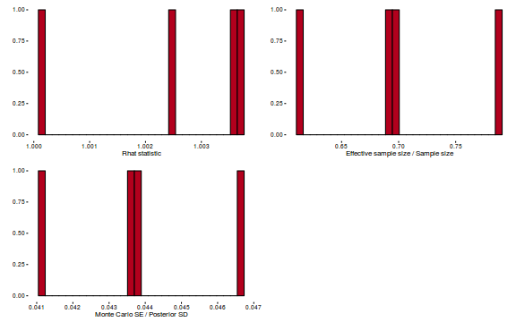
- Trace plots
- Explore the model fit diagnostics.
- Explore the patterns in simulated residuals:
Show code
lambda.brm = exp(fitted(limpets.brm, scale='linear', summary=FALSE))[,1:nrow(limpets)] theta = binomial()$linkinv(mean(rstan:::extract(limpets.brm$fit, 'b_spec')[[1]])) simRes(lambda.brm, limpets$Count, family='zip', theta=theta)
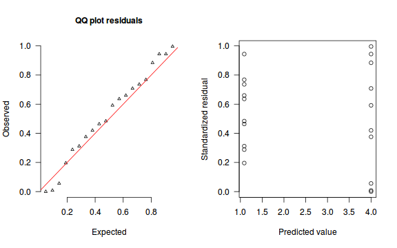
[1] 0.660 0.484 0.944 0.464 0.288 0.196 0.736 0.312 0.768 0.636 0.592 0.996 0.376 0.056 0.420 0.008 0.000 0.884 0.944 0.708
- Goodness of fit test:
Show code
## Poisson Resid.brm <- residuals(limpets.brm, type='pearson', summary=FALSE) SSres.brm <- apply(Resid.brm^2,1,sum) lambda.brm = fitted(limpets.brm, scale='response', summary=FALSE) YNew.brm <- matrix(rpois(length(lambda.brm), lambda=lambda.brm),nrow=nrow(lambda.brm)) Resid1.brm<-(lambda.brm - YNew.brm)/sqrt(lambda.brm) SSres.sim.brm<-apply(Resid1.brm^2,1,sum) mean(SSres.sim.brm>SSres.brm)
[1] 0.07466667
- Fitted and observed values (plot):
Show code
newdata <- data.frame(Shore=levels(limpets$Shore)) tempdata = fitted(limpets.brm, scale='response',newdata=newdata) tempdata <- cbind(newdata, Mean=tempdata[,'Estimate'], Lower=tempdata[,'2.5%ile'], Upper=tempdata[,'97.5%ile']) library(ggplot2) ggplot(limpets, aes(y=Count, x=Shore)) + geom_boxplot() + geom_pointrange(data=tempdata,aes(y=Mean, ymin=Lower, ymax=Upper), color='red')
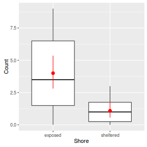
##OR the manual way Xmat <- model.matrix(~Shore, data=newdata) coefs <- as.matrix(as.data.frame(rstan:::extract(limpets.brm$fit))) coefs <- coefs[,grep('^b_main', colnames(coefs))] fit = exp(coefs %*% t(Xmat)) tempdata <- cbind(newdata, plyr:::adply(fit, 2, function(x) { data.frame(Mean=mean(x), Median=median(x), HPDinterval(as.mcmc(x))) })) ggplot(limpets, aes(y=Count, x=Shore)) + geom_boxplot() + geom_pointrange(data=tempdata,aes(y=Mean, ymin=lower, ymax=upper), color='red')

- Check for overdispersion:
Show code
coefs <- as.matrix(as.data.frame(rstan:::extract(limpets.brm$fit))) coefs <- coefs[,grep('^b_', colnames(coefs))] Resid <- residuals(limpets.brm, type='pearson',summary=FALSE) RSS <- apply(Resid^2,1,sum) Disp <- RSS/(nrow(limpets)-ncol(coefs)) data.frame(Median=median(Disp), Mean=mean(Disp), HPDinterval(as.mcmc(Disp)))
Median Mean lower upper var1 1.750797 1.789582 1.686107 2.004651
- Explore the patterns in simulated residuals:
-
Given that the model seems to be well specified and there are no diagnostics that would question the
reliability of the model, lets explore the model parameters.
Show code
summary(limpets.brm)
Family: zero_inflated_poisson (log) Formula: Count ~ 0 + spec + main + main:Shore Data: limpets (Number of observations: 20) Samples: 3 chains, each with iter = 2000; warmup = 1000; thin = 4; total post-warmup samples = 750 WAIC: Not computed Fixed Effects: Estimate Est.Error l-95% CI u-95% CI Eff.Sample Rhat spec -787.73 602.86 -2246.33 -35.06 459 1 main 1.37 0.16 1.03 1.68 520 1 main:Shoresheltered -1.33 0.34 -2.00 -0.70 590 1 Samples were drawn using sampling(NUTS). For each parameter, Eff.Sample is a crude measure of effective sample size, and Rhat is the potential scale reduction factor on split chains (at convergence, Rhat = 1).exp(coef(limpets.brm))
mean spec 0.0000000 main 3.9513940 main:Shoresheltered 0.2637503
coefs <- as.matrix(as.data.frame(rstan:::extract(limpets.brm$fit))) coefs <- coefs[,grep('^b_', colnames(coefs))] plyr:::adply(exp(coefs), 2, function(x) { data.frame(Mean=mean(x), median=median(x), HPDinterval(as.mcmc(x))) })
X1 Mean median lower upper 1 b_spec 5.746643e-08 3.422828e-287 0.0000000 1.358137e-28 2 b_main 4.000980e+00 3.973522e+00 2.8246056 5.369929e+00 3 b_main.Shoresheltered 2.787194e-01 2.671325e-01 0.1166521 4.613737e-01
marginal_effects(limpets.brm)
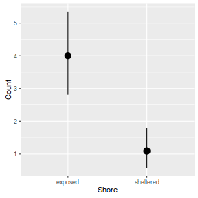
- Estimate the strength of the relationship
Show code
## calculate the expected values on the response scale lambda.brm = fitted(limpets.brm, scale='response', summary=FALSE) ## calculate the raw SSresid SSres.brm <- apply((-1*(sweep(lambda.brm,2, limpets$Count,'-')))^2,1,sum) SSres.null <- sum((limpets$Count - mean(limpets$Count))^2) #OR #calculate the model r2 1-mean(SSres.brm)/SSres.null
[1] 0.2554819
#OR manually coefs <- as.matrix(as.data.frame(rstan:::extract(limpets.brm$fit))) coefs <- coefs[,grep('^b_main', colnames(coefs))] Xmat <- model.matrix(~Shore, data=limpets) lambda.brm = exp(coefs %*% t(Xmat)) ## calculate the raw SSresid SSres.brm <- apply((-1*(sweep(lambda.brm,2,limpets$Count,'-')))^2,1,sum) SSres.null <- crossprod(limpets$Count - mean(limpets$Count)) #calculate the model r2 1-mean(SSres.brm)/SSres.null
[,1] [1,] 0.2554819
## Alternatively.. R.var = apply(residuals(limpets.brm, summary=FALSE),1,var) X.var = apply(fitted(limpets.brm, summary=FALSE),1,var) R2.marginal <- X.var/(X.var + R.var) data.frame(Median=median(R2.marginal), coda:::HPDinterval(as.mcmc(R2.marginal)))
Median lower upper var1 0.2907571 0.1057379 0.4574874
- Produce a suitable summary plot
Show code
coefs <-as.matrix(as.data.frame(rstan:::extract(limpets.brm$fit))) coefs <- coefs[,grep('^b_main', colnames(coefs))] newdata <- data.frame(Shore=levels(limpets$Shore)) Xmat <- model.matrix(~Shore, data=newdata) fit = exp(coefs %*% t(Xmat)) newdata = cbind(newdata, plyr:::adply(fit, 2, function(x) { data.frame(Mean=mean(x, na.rm=TRUE),Median=median(x, na.rm=TRUE), HPDinterval(as.mcmc(x))) })) ggplot(limpets, aes(y=Count, x=Shore)) + geom_point(color='grey') + geom_pointrange(data=newdata, aes(y=Mean, ymin=lower, ymax=upper)) + scale_y_continuous('Abundance of limpets') + scale_x_discrete('Shore type') + theme_classic() + theme(axis.line.x=element_line(), axis.line.y=element_line())
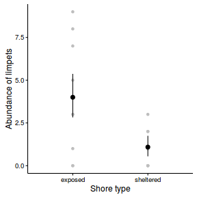
- Since it is difficult to diagnose many issues from the typical residuals we will now explore simulated residuals.
- Since it is difficult to diagnose many issues from the typical residuals we will now explore simulated residuals.
