Tutorial 12.10 - Integrated Nested Laplace Approximation (INLA) for (generalized) linear models
25 Feb 2016
Overview
Tutorial 12.9 introduced the basic INLA framework as well as a fully fleshed out example using a fabricated data set. The current tutorial will focus on linear models and using both fabricated data and real worked examples.
In this tutorial we have an opportunity to explore INLA for multilevel (hierarchical) models.Although performing very simple linear regression with INLA might be seen as a complete overkill (as it does not really utilize the main features for which INLA is designed), from a pedagogical perspective, starting with simpler models for which robust and well understood solutions exist allows us to gradually build up an understanding of how INLA works. Model complexity can be gradually introduced, thereby allowing us to explore techniques progressively by building on more solid foundations. All data sets will be fabricated from set parameters so that we always have a 'truth' from which to compare outcomes and as a point of comparison, each data set will be followed by Frequentist and Bayesian MCMC outcomes.
Simple regression
library(R2jags)
library(INLA)
library(ggplot2)
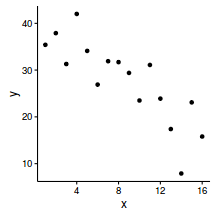
Lets say we had set up an experiment in which we applied a continuous treatment ($x$) ranging in magnitude from 0 to 16 to a total of 16 sampling units ($n=16$) and then measured a response ($y$) from each unit. As this section is mainly about the generation of artificial data (and not specifically about what to do with the data), understanding the actual details are optional and can be safely skipped. Consequently, I have folded (toggled) this section away.
- the sample size = 16
- the continuous $x$ variable ranging from 0 to 16
- when the value of $x$ is 0, $y$ is expected to be 40 ($\beta_0=40$)
- a 1 unit increase in $x$ is associated with a 1.5 unit decline in $y$ ($\beta_1=-1.5$)
- the data are drawn from normal distributions with a mean of 0 and standard deviation of 5 ($\sigma^2=25$)
set.seed(1)
n <- 16
a <- 40  #intercept
b <- -1.5  #slope
sigma2 <- 25  #residual variance (sd=5)
x <- 1:n  #values of the year covariate
eps <- rnorm(n, mean = 0, sd = sqrt(sigma2))  #residuals
y <- a + b * x + eps  #response variable
#OR
y <- (model.matrix(~x) %*% c(a,b))+eps
data <- data.frame(y=round(y,1), x)  #dataset
head(data)  #print out the first six rows of the data set
     y x
1 35.4 1
2 37.9 2
3 31.3 3
4 42.0 4
5 34.1 5
6 26.9 6
ggplot(data, aes(y=y, x=x)) + geom_point() + theme_classic()
$$ y_i = \alpha + \beta x_i + \varepsilon_i \hspace{4em}\varepsilon_i\sim{}\mathcal{N}(0, \sigma^2) $$
summary(lm(y~x, data=data))
Call:
lm(formula = y ~ x, data = data)

Residuals:
     Min       1Q   Median       3Q      Max
-11.3694  -3.5053   0.6239   2.6522   7.3909

Coefficients:
            Estimate Std. Error t value Pr(>|t|)
(Intercept)  40.7450     2.6718  15.250 4.09e-10 ***
x            -1.5340     0.2763  -5.552 7.13e-05 ***
---
Signif. codes:  0 '***' 0.001 '**' 0.01 '*' 0.05 '.' 0.1 ' ' 1

Residual standard error: 5.095 on 14 degrees of freedom
Multiple R-squared:  0.6876,	Adjusted R-squared:  0.6653
F-statistic: 30.82 on 1 and 14 DF,  p-value: 7.134e-05
confint(lm(y~x, data=data))
                2.5 %     97.5 %
(Intercept) 35.014624 46.4753756
x           -2.126592 -0.9413493
modelString="
model {
   #Likelihood
   for (i in 1:n) {
      y[i]~dnorm(mu[i],tau)
      mu[i] <- alpha+beta*x[i]
   }

   #Priors
   alpha ~ dnorm(0,1.0E-6)
   beta ~ dnorm(0,1.0E-6)
   tau <- 1 / (sigma * sigma)
   sigma~dgamma(0.1,0.001)
   #tau <- exp(log.tau)
   #log.tau ~ dgamma(1,0.01)
 }
"
data.list <- with(data, list(y=y, x=x, n=nrow(data)))
data.jags <- jags(data=data.list,
           inits=NULL,
           parameters.to.save=c('alpha','beta', 'sigma'),
           model.file=textConnection(modelString),
           n.chains=3,
           n.iter=100000,
           n.burnin=20000,
                   n.thin=100
           )
Compiling model graph
   Resolving undeclared variables
   Allocating nodes
   Graph Size: 75

Initializing model
print(data.jags)
Inference for Bugs model at "5", fit using jags,
 3 chains, each with 1e+05 iterations (first 20000 discarded), n.thin = 100
 n.sims = 2400 iterations saved
         mu.vect sd.vect   2.5%    25%    50%    75%   97.5%  Rhat n.eff
alpha     40.813   2.837 35.375 38.950 40.766 42.656  46.533 1.001  2400
beta      -1.540   0.291 -2.119 -1.729 -1.536 -1.344  -0.973 1.001  2400
sigma      5.383   1.089  3.739  4.600  5.195  6.001   7.939 1.000  2400
deviance  98.660   2.585 95.609 96.706 98.040 99.958 105.200 1.001  2300

For each parameter, n.eff is a crude measure of effective sample size,
and Rhat is the potential scale reduction factor (at convergence, Rhat=1).

DIC info (using the rule, pD = var(deviance)/2)
pD = 3.3 and DIC = 102.0
DIC is an estimate of expected predictive error (lower deviance is better).
data.inla <- inla(y~x, data=data, control.compute=list(dic=TRUE, cpo=TRUE, waic=TRUE))
The inla() function returns an object of class inla of which there are two methods available (summary and plot). For an inla fitted model, the summary method returns the Fixed and Random effects as well as a number of information criterion and limited fit diagnostics.
summary(data.inla)
Call:
c("inla(formula = y ~ x, data = data, control.compute = list(dic = TRUE, ",  "    cpo = TRUE, waic = TRUE))")

Time used:
 Pre-processing    Running inla Post-processing           Total
         0.1013          0.0632          0.0360          0.2006

Fixed effects:
               mean     sd 0.025quant 0.5quant 0.975quant    mode kld
(Intercept) 40.7441 2.5688    35.6573  40.7440    45.8219 40.7442   0
x           -1.5339 0.2657    -2.0599  -1.5339    -1.0087 -1.5339   0

The model has no random effects

Model hyperparameters:
                                          mean     sd 0.025quant 0.5quant 0.975quant   mode
Precision for the Gaussian observations 0.0438 0.0155     0.0199   0.0418     0.0798 0.0378

Expected number of effective parameters(std dev): 2.00(0.00)
Number of equivalent replicates : 8.00

Deviance Information Criterion (DIC) ...: 100.64
Effective number of parameters .........: 2.634

Watanabe-Akaike information criterion (WAIC) ...: 101.40
Effective number of parameters .................: 2.942

Marginal log-Likelihood:  -64.55
CPO and PIT are computed

Posterior marginals for linear predictor and fitted values computed
Lets focus on the different components of this output. The 'Fixed' effects represent a set of summaries from the posterior distribution. These results are very similar to those yielded from the Frequentist and Bayesian MCMC approaches.
               mean     sd 0.025quant 0.5quant 0.975quant    mode kld
(Intercept) 40.7441 2.5688    35.6573  40.7440    45.8219 40.7442   0
x           -1.5339 0.2657    -2.0599  -1.5339    -1.0087 -1.5339   0
                                          mean     sd 0.025quant 0.5quant 0.975quant   mode
Precision for the Gaussian observations 0.0438 0.0155     0.0199   0.0418     0.0798 0.0378
Expected number of effective parameters(std dev): 2.00(0.00)
Number of equivalent replicates : 8.00
The number of equivalent replicates is the number of replicates (sample size) per effective parameter. In this case, there are 16 observations, so there are $16/2=8$ equivalent replicates. Low values (relative to the overall sample size) are indicative of a poor fit.
Out-of-sample or leave-one-out predictive performance
Arguably, the best way to assess the fit of a model is via an estimate of the models predictive accuracy, the gold standard of which is out-of-sample estimation via cross-validation (in which each observed response is compared to a prediction derived from a model that trained on without the focal response value). However, as this approach required repeated model fits, it is not overly practical for large complex models, MCMC simulations or very sparse data. Traditional alternatives to cross-validation include Akaike's Information Criterion (AIC) and Deviance Information Criterion (DIC) when associated with Bayesian analyses.
Deviance Information Criterion (DIC)...: 100.64
Effective number of parameters .........: 2.634
Watanabe-Akaike information criterion (WAIC) ...: 101.40
Effective number of parameters .................: 2.942
The effective number of parameters (pD) is the posterior mean deviance minus the deviance measured at the posterior mean of the parameters. Both the DIC and pD are similar to those reported by JAGS.
Wantanabe-Akaike Information Criterion or Widely Applicable Information Criterion (WAIC). By contrast to AIC (and DIC) WAIC is a more fully Bayesian approach for estimating the out-of-sample expectation based on the log pointwise posterior predictive density.
Two additional out-of-sample estimates (measures of fit) supported by INLA include:
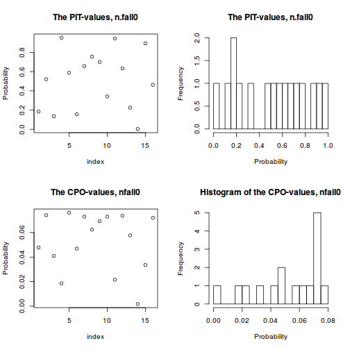
- Conditional Predictive Ordinate (CPO) is the density of the observed value of $y_i$ within the out-of-sample ($y_{-i}$) posterior predictive distribution.
A small CPO value associated with an observation suggests that this observation is unlikely (or surprising) in light of the model, priors and other
data in the model. In addition, the sum of the CPO values (or alternatively, the negative of the mean natural logarithm of the CPO values) is a measure of fit.
In this case there are no CPO values that are considerably smaller (order of magnitude smaller) than the others - so with respect to the model, none of the observed values would be considered 'surprising'. Various assumptions are made behind INLA's computations. If any of these assumptions fail of an observation, it is flagged within (in this case) cpo$failure as a non-zero. When this is the case, it is prudent to recalculate the CPO values after removing the observations associated with failure flags not equal to zero and re-fitting the model. This can be performed using the inla.cpo() function.
data.inla$cpo$cpo
 [1] 0.047749222 0.074109301 0.041001671 0.018540996 0.076175384 0.046941565 0.073009041 0.062423313
 [9] 0.069163109 0.072927701 0.021584385 0.073660042 0.057706132 0.001797082 0.033613593 0.071977093
sum(data.inla$cpo$cpo)
[1] 0.8423796
-mean(log(data.inla$cpo$cpo))
[1] 3.173897
In this case, there are no non-zero CPO values.data.inla$cpo$failure
[1] 0 0 0 0 0 0 0 0 0 0 0 0 0 0 0 0
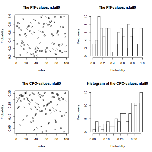
- Probability Integral Transforms (PIT) provides a version of CPO that is calibrated to the level of the Gaussian field so that it is clearer
whether or not any of the values are 'small' (all values must be between 0 and 1). A histogram of PIT values that does not look approximately uniform (flat) indicates a lack of model fit.
In this case the PIT values do not appear to deviate from a uniform distribution and thus do not indicate a lack of fit.
plot(data.inla, plot.fixed.effects=FALSE, plot.lincomb=FALSE, plot.random.effects=FALSE,
     plot.hyperparameters=FALSE, plot.predictor=FALSE, plot.q=FALSE, plot.cpo=TRUE,
     single=FALSE)
The influence of priors
When fitting the INLA model above, we did not specify priors. Consequently, the default priors were employed. To review what these priors are, we can use the inla.show.hyperspec() function - which returns a list containing information about all the hyper-priors used in a model.
inla.show.hyperspec(data.inla)
List of 3
 $ predictor:List of 1
    $ hyper:List of 1
       $ theta:List of 8
          $ name      : atomic [1:1] log precision
          $ short.name: atomic [1:1] prec
          $ initial   : atomic [1:1] 11
          $ fixed     : atomic [1:1] TRUE
          $ prior     : atomic [1:1] loggamma
          $ param     : atomic [1:2] 1e+00 1e-05
 $ family   :List of 1
    $ :List of 3
       $ label: chr "gaussian"
       $ hyper:List of 1
          $ theta:List of 8
             $ name      : atomic [1:1] log precision
             $ short.name: atomic [1:1] prec
             $ initial   : atomic [1:1] 4
             $ fixed     : atomic [1:1] FALSE
             $ prior     : atomic [1:1] loggamma
             $ param     : atomic [1:2] 1e+00 5e-05
       $ link :List of 1
          $ hyper: list()
 $ fixed    :List of 2
    $ :List of 3
       $ label     : chr "(Intercept)"
       $ prior.mean: num 0
       $ prior.prec: num 0
    $ :List of 3
       $ label     : chr "x"
       $ prior.mean: num 0
       $ prior.prec: num 0.001
In order to drive the specification of weekly informative priors for variance components (a prior that allows the data to dictate the parameter estimates whilst constraining the range of the marginal distribution within sensible bounds), we can consider the range over which the marginal distribution of variance components would be sensible. For the range [-R,R], the equivalent gamma parameters: $$ \begin{align} a &= \frac{d}{2}\\ b &= \frac{R^2d}{2*(t^d_{1-(1-q)/2})^2} \end{align} $$ where $d$ is the degrees of freedom (for Cauchy marginal, $d=1$) and $t^d_{1-(1-q)/2}$ is the $q$th quantile of a Student $t$ with $d$ degrees of freedom. Hence if we considered variance likely to be in the range of [0,10], we could define a loggamma prior of: $$ \begin{align} a &= \frac{1}{2} = 0.5\\ b &= \frac{10^2}{2*161.447} = 0.31\\ \tau &\sim{} log\Gamma(0.5,0.31) \end{align} $$
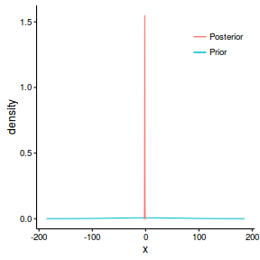
The priors for the fixed effects (intercept and slope) are both Normal distributions
with mean of 0 and precision (0.001). This implies that the prior for slope has a standard deviation
of approximately 31 (since $\sigma = \frac{1}{\sqrt{\tau}}$). As a general rule, three standard deviations
envelopes most of a distribution, and thus this prior defines a distribution whose density is almost entirely
within the range [-93,93]. Whilst this might be appropriate
for the intercept, it is arguably very wide for the slope given the range of the predictor variable.
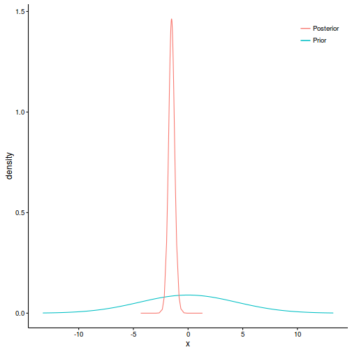
In order to generate realistic informative Gaussian priors (for the purpose of constraining the posterior to a logical range) for fixed parameters, the following formulae are useful: $$ \begin{align} \mu &= \frac{z_2\theta_1 - z_1\theta_2}{z_2-z_1}\\ \sigma &= \frac{\theta_2 - \theta_1}{z_2-z_1} \end{align} $$ where $\theta_1$ and $\theta_2$ are the quantiles on the response scale and $z_1$ and $z_2$ are the corresponding quantiles on the standard normal scale. Hence, if we considered that the slope is likely to be in the range of [-10,10], we could specify a Normal prior with mean of ($\mu=\frac{(qnorm(0.5,0,1)*0) - (qnorm(0.975,0,1)*10)}{10-0} = 0$) and a standard deviation of ($\mu=\frac{10 - 0}{qnorm(0.975,0,1)-qnorm(0.5,0,1)} = 5.102$). In INLA (which defines priors in terms of precision rather than standard deviation), the associated prior would be $\beta \sim{} \mathcal{N}(0, 0.196)$.
Lets plot the prior and posterior for slope.
#the default priors specify a standard deviation of:
(SD<-(1/sqrt(0.001) * qnorm(0.975,0,1)))
[1] 61.9795
prior <- data.frame(x=seq(-3*SD,3*SD,len=1000))
prior$density <- dnorm(prior$x,0,SD)
post <- data.frame(data.inla$marginals.fixed[[2]])
head(post)
          x            y
1 -4.190463 1.765936e-16
2 -3.659143 9.807886e-11
3 -3.127823 1.422271e-06
4 -2.862163 6.240289e-05
5 -2.596503 1.483329e-03
6 -2.330843 2.134545e-02
ggplot(prior, aes(y=density, x=x)) + geom_line(aes(color='Prior')) +
       geom_line(data=post, aes(y=y, x=x, color='Posterior')) +
       scale_color_discrete('')+
       theme_classic()+theme(legend.position=c(1,1), legend.justification=c(1,1))
s <- inla.contrib.sd(data.inla, nsamples = 1000)
s$hyper
                                     mean        sd     2.5%    97.5%
sd for the Gaussian observations 4.991154 0.9202552 3.527553 7.121831
data.inla <- inla(y~x, data=data, control.compute=list(dic=TRUE, cpo=TRUE, waic=TRUE),
                  control.fixed=list(mean=0, prec=0.196, mean.intercept=0, prec.intercept=0.001),
                  control.family=list(hyper=list(prec=list(prior='loggamma', param=c(0.1,0.1)))))
summary(data.inla)
Call:
c("inla(formula = y ~ x, data = data, control.compute = list(dic = TRUE, ",  "    cpo = TRUE, waic = TRUE), control.family = list(hyper = list(prec = list(prior = \"loggamma\", ",  "    param = c(0.1, 0.1)))), control.fixed = list(mean = 0, prec = 0.196, ",  "    mean.intercept = 0, prec.intercept = 0.001))")

Time used:
 Pre-processing    Running inla Post-processing           Total
         0.0911          0.0326          0.0285          0.1523

Fixed effects:
               mean     sd 0.025quant 0.5quant 0.975quant    mode kld
(Intercept) 40.2459 2.7140    34.8045  40.2675    45.5553 40.3057   0
x           -1.4833 0.2804    -2.0322  -1.4855    -0.9215 -1.4894   0

The model has no random effects

Model hyperparameters:
                                          mean     sd 0.025quant 0.5quant 0.975quant   mode
Precision for the Gaussian observations 0.0388 0.0146     0.0167   0.0368      0.073 0.0328

Expected number of effective parameters(std dev): 1.977(0.0069)
Number of equivalent replicates : 8.092

Deviance Information Criterion (DIC) ...: 100.79
Effective number of parameters .........: 2.636

Watanabe-Akaike information criterion (WAIC) ...: 101.14
Effective number of parameters .................: 2.604

Marginal log-Likelihood:  -56.99
CPO and PIT are computed

Posterior marginals for linear predictor and fitted values computed
data.inla <- inla(y~x, data=data, control.compute=list(dic=TRUE, cpo=TRUE, waic=TRUE),
                  control.fixed=list(mean=0, prec=0.0196, mean.intercept=0, prec.intercept=0.001),
                  control.family=list(hyper=list(prec=list(prior='loggamma', param=c(0.1,0.1)))))
summary(data.inla)
Call:
c("inla(formula = y ~ x, data = data, control.compute = list(dic = TRUE, ",  "    cpo = TRUE, waic = TRUE), control.family = list(hyper = list(prec = list(prior = \"loggamma\", ",  "    param = c(0.1, 0.1)))), control.fixed = list(mean = 0, prec = 0.0196, ",  "    mean.intercept = 0, prec.intercept = 0.001))")

Time used:
 Pre-processing    Running inla Post-processing           Total
         0.0923          0.0239          0.0286          0.1448

Fixed effects:
               mean     sd 0.025quant 0.5quant 0.975quant    mode kld
(Intercept) 40.4222 2.7267    34.9757  40.4364    45.7778 40.4616   0
x           -1.5041 0.2822    -2.0593  -1.5054    -0.9414 -1.5077   0

The model has no random effects

Model hyperparameters:
                                          mean     sd 0.025quant 0.5quant 0.975quant   mode
Precision for the Gaussian observations 0.0388 0.0146     0.0167   0.0368      0.073 0.0328

Expected number of effective parameters(std dev): 1.991(0.0028)
Number of equivalent replicates : 8.036

Deviance Information Criterion (DIC) ...: 100.80
Effective number of parameters .........: 2.651

Watanabe-Akaike information criterion (WAIC) ...: 101.16
Effective number of parameters .................: 2.62

Marginal log-Likelihood:  -57.94
CPO and PIT are computed

Posterior marginals for linear predictor and fitted values computed
s <- inla.contrib.sd(data.inla, nsamples = 1000)
s$hyper
                                     mean       sd     2.5%    97.5%
sd for the Gaussian observations 5.337874 1.088706 3.663546 7.863846
#the default priors specify a standard deviation of:
(SD<-(1/sqrt(0.196) * qnorm(0.975,0,1)))
[1] 4.427107
prior <- data.frame(x=seq(-3*SD,3*SD,len=1000))
prior$density <- dnorm(prior$x,0,SD)
post <- data.frame(data.inla$marginals.fixed[[2]])
head(post)
          x            y
1 -4.325697 2.134404e-16
2 -3.761375 1.037706e-10
3 -3.197053 1.349437e-06
4 -2.914892 5.713188e-05
5 -2.632731 1.331189e-03
6 -2.350570 1.925008e-02
ggplot(prior, aes(y=density, x=x)) + geom_line(aes(color='Prior')) +
       geom_line(data=post, aes(y=y, x=x, color='Posterior')) +
       scale_color_discrete('')+
       theme_classic()+theme(legend.position=c(1,1), legend.justification=c(1,1))
More detailed information
In addition to the PIT and CPO distributions, there are numerous other summary plots available, each of which summarizes the marginal distribution of the different types of model parameters (fixed, random, hyper-parameters etc) and predictions. These can be produced in one hit using the plot() function. However, I will produce them individually in order to assist discussion. Moreover, as a result of complexities arising from the need for the plot() function to work in Rstudio, INLA's plot() function and knitr are slightly incompatible at the moment...
Additionally, the fitted INLA object (a list) contains a large number of items, each of which capture different aspects of the approximated parameters.
names(data.inla)
 [1] "names.fixed"                 "summary.fixed"               "marginals.fixed"
 [4] "summary.lincomb"             "marginals.lincomb"           "size.lincomb"
 [7] "summary.lincomb.derived"     "marginals.lincomb.derived"   "size.lincomb.derived"
[10] "mlik"                        "cpo"                         "po"
[13] "waic"                        "model.random"                "summary.random"
[16] "marginals.random"            "size.random"                 "summary.linear.predictor"
[19] "marginals.linear.predictor"  "summary.fitted.values"       "marginals.fitted.values"
[22] "size.linear.predictor"       "summary.hyperpar"            "marginals.hyperpar"
[25] "internal.summary.hyperpar"   "internal.marginals.hyperpar" "offset.linear.predictor"
[28] "model.spde2.blc"             "summary.spde2.blc"           "marginals.spde2.blc"
[31] "size.spde2.blc"              "model.spde3.blc"             "summary.spde3.blc"
[34] "marginals.spde3.blc"         "size.spde3.blc"              "logfile"
[37] "misc"                        "dic"                         "mode"
[40] "neffp"                       "joint.hyper"                 "nhyper"
[43] "version"                     "Q"                           "graph"
[46] "ok"                          "cpu.used"                    "all.hyper"
[49] ".args"                       "call"                        "model.matrix"
This is obviously a very large list. In order to make more sense of all that is available, we can group the returned INLA list into functional categories:
- parameter estimates
INLA object Description names.fixed the names of fixed effects parameters summary.fixed summaries (mean, standard deviation and quantiles) of fixed posteriors (on link scale) marginals.fixed list of posterior marginal densities of the fixed effects size.random number of levels of each of the structured random covariates summary.random summaries (mean, standard deviation and quantiles) of the structured random effects (smoothers etc) marginals.random list of posterior marginal densities of the random effects summary.hyperpar summaries (mean, standard deviation and quantiles) of the model hyper-parameters (precision, overdispersion, correlation etc) marginals.hyperpar list of posterior marginal densities of the model hyper-parameters - predictions and contrasts
INLA object Description model.matrix model matrix of the fixed effects - a row for each row of the input data summary.linear.predictor summaries (mean, standard deviation and quantiles) of the linear predictor - a prediction (on the link scale) associated with each row of the input data marginals.linear.predictor list of posterior marginal densities of the linear predictor summary.fitted.values summaries (mean, standard deviation and quantiles) of the fitted values - a prediction (on the response scale) associated with each row of the input data marginals.fitted.values list of posterior marginal densities of the fitted values summary.lincomb summaries (mean, standard deviation and quantiles) of the defined linear combinations (on the link scale) marginals.lincomb list of posterior marginal densities of the defined linear combinations summary.lincomb.derived summaries (mean, standard deviation and quantiles) of the defined linear combinations (on the response scale) marginals.lincomb.derived list of posterior marginal densities of the defined linear combinations (response scale) - model performance measures
INLA object Description mlik log marginal likelihood of the model (when mlik=TRUE) dic deviance information criterion of the model (when dic=TRUE) waic Watanabe-Akaike (Widely Applicable) information criterion of the model (when dic=TRUE) neffp expected number of parameters (and standard deviation) and number of replicates per parameter in the model cpo conditional predictive ordinate (cpo), probability integral transform (pit) and vector of assumption failures (failures) of the model (when cpo=TRUE)
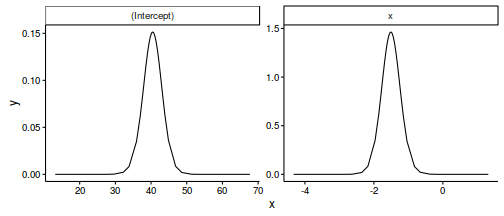
Fixed effects
plot(data.inla, plot.fixed.effects = TRUE, plot.lincomb = FALSE, plot.random.effects = FALSE, plot.hyperparameters = FALSE,
    plot.predictor = FALSE, plot.q = FALSE, plot.cpo = FALSE, single = FALSE)
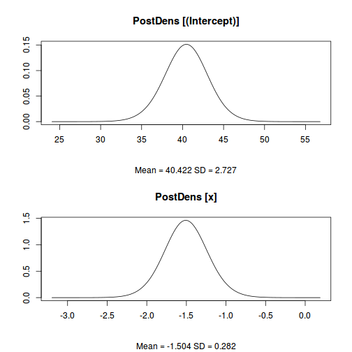
data.inla$summary.fixed
                 mean        sd 0.025quant  0.5quant 0.975quant      mode          kld
(Intercept) 40.422174 2.7267362   34.97573 40.436435 45.7778033 40.461613 3.011495e-11
x           -1.504087 0.2821624   -2.05931 -1.505424 -0.9413974 -1.507741 2.972068e-11
data.inla$marginals.fixed
$`(Intercept)`
             x            y
 [1,] 13.15496 4.410151e-17
 [2,] 18.60840 1.905779e-11
 [3,] 24.06185 2.152067e-07
 [4,] 26.78857 8.435060e-06
 [5,] 29.51529 1.784278e-04
 [6,] 32.24201 2.276125e-03
 [7,] 33.83266 8.280310e-03
 [8,] 35.92316 3.499961e-02
 [9,] 36.96775 6.200022e-02
[10,] 37.65244 8.427154e-02
[11,] 38.19117 1.028661e-01
[12,] 38.64056 1.178672e-01
[13,] 39.04390 1.299800e-01
[14,] 39.41565 1.392874e-01
[15,] 39.76649 1.459042e-01
[16,] 40.10455 1.499193e-01
[17,] 40.27099 1.509687e-01
[18,] 40.43643 1.513822e-01
[19,] 40.60209 1.511608e-01
[20,] 40.76790 1.503044e-01
[21,] 41.10458 1.466640e-01
[22,] 41.45260 1.404086e-01
[23,] 41.81934 1.314582e-01
[24,] 42.21872 1.195765e-01
[25,] 42.66654 1.045571e-01
[26,] 43.18698 8.627934e-02
[27,] 43.85476 6.385703e-02
[28,] 44.86945 3.628873e-02
[29,] 46.88034 8.629793e-03
[30,] 48.60235 1.975121e-03
[31,] 51.32907 1.352744e-04
[32,] 54.05579 5.756324e-06
[33,] 56.78251 1.349249e-07
[34,] 62.23596 1.021137e-11
[35,] 67.68940 2.068547e-17

$x
                x            y
 [1,] -4.32569687 2.134404e-16
 [2,] -3.76137496 1.037706e-10
 [3,] -3.19705306 1.349437e-06
 [4,] -2.91489210 5.713188e-05
 [5,] -2.63273115 1.331189e-03
 [6,] -2.35057020 1.925008e-02
 [7,] -2.17334332 8.304301e-02
 [8,] -1.96491059 3.492400e-01
 [9,] -1.85981324 6.148759e-01
[10,] -1.79056620 8.315525e-01
[11,] -1.73580056 1.011021e+00
[12,] -1.69001537 1.154394e+00
[13,] -1.64879258 1.269090e+00
[14,] -1.61067721 1.356196e+00
[15,] -1.57459777 1.416978e+00
[16,] -1.53973520 1.452399e+00
[17,] -1.52252620 1.460799e+00
[18,] -1.50542406 1.463031e+00
[19,] -1.48827869 1.459127e+00
[20,] -1.47107359 1.449088e+00
[21,] -1.43609861 1.410468e+00
[22,] -1.39985194 1.346777e+00
[23,] -1.36155020 1.257371e+00
[24,] -1.31985206 1.140529e+00
[25,] -1.27276242 9.936500e-01
[26,] -1.21787798 8.165285e-01
[27,] -1.14702386 6.008029e-01
[28,] -1.03864956 3.384795e-01
[29,] -0.82220815 7.976568e-02
[30,] -0.65760448 2.185504e-02
[31,] -0.37544353 1.705125e-03
[32,] -0.09328257 8.038838e-05
[33,]  0.18887838 2.048111e-06
[34,]  0.75320028 1.812337e-10
[35,]  1.31752219 4.198486e-16
library(dplyr)
data.inla.fixed <- reshape2:::melt(data.inla$marginals.fixed) %>%
                   reshape2:::dcast(L1+Var1~Var2, value='value')
ggplot(data.inla.fixed, aes(y=y, x=x)) + geom_line() +
      facet_wrap(~L1, scales='free', nrow=1) + theme_classic()
Predictor
plot(data.inla, plot.fixed.effects=FALSE, plot.lincomb=FALSE, plot.random.effects=FALSE,
     plot.hyperparameters=FALSE, plot.predictor=TRUE, plot.q=FALSE, plot.cpo=FALSE,
     single=FALSE)
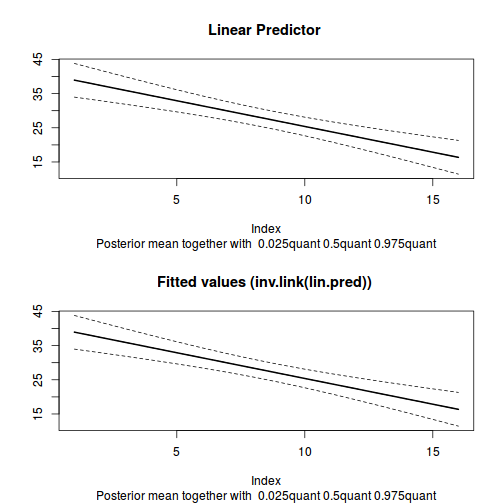
data.inla$summary.linear.predictor
                 mean       sd 0.025quant 0.5quant 0.975quant     mode          kld
predictor.01 38.91874 2.483244   33.96448 38.93146   43.79792 38.95390 1.007436e-07
predictor.02 37.41459 2.247989   32.92995 37.42602   41.83181 37.44617 1.014385e-07
predictor.03 35.91045 2.024777   31.87159 35.92057   39.88955 35.93843 1.027624e-07
predictor.04 34.40632 1.818051   30.78060 34.41514   37.97993 34.43071 1.051053e-07
predictor.05 32.90219 1.634077   29.64458 32.90971   36.11533 32.92298 1.090693e-07
predictor.06 31.39807 1.481359   28.44673 31.40428   34.31258 31.41524 1.154613e-07
predictor.07 29.89397 1.370386   27.16634 29.89887   32.59239 29.90751 1.250763e-07
predictor.08 28.38989 1.311798   25.78241 28.39345   30.97613 28.39978 1.380414e-07
predictor.09 26.88582 1.312630   24.28112 26.88804   29.47847 26.89203 1.530650e-07
predictor.10 25.38177 1.372775   22.66255 25.38262   28.09812 25.38426 1.678379e-07
predictor.11 23.87775 1.485046   20.93976 23.87723   26.82085 23.87651 1.806989e-07
predictor.12 22.37373 1.638769   19.13512 22.37184   25.62556 22.36874 1.923988e-07
predictor.13 20.86972 1.823489   17.26929 20.86646   24.49158 20.86098 2.011791e-07
predictor.14 19.36572 2.030767   15.35897 19.36108   23.40225 19.35322 2.077685e-07
predictor.15 17.86174 2.254388   13.41636 17.85572   22.34529 17.84548 2.126772e-07
predictor.16 16.35775 2.489953   11.45012 16.35035   21.31196 16.33773 2.163935e-07
data.inla$summary.fitted.values
                        mean       sd 0.025quant 0.5quant 0.975quant     mode
fitted.predictor.01 38.91874 2.483244   33.96448 38.93146   43.79792 38.95390
fitted.predictor.02 37.41459 2.247989   32.92995 37.42602   41.83181 37.44617
fitted.predictor.03 35.91045 2.024777   31.87159 35.92057   39.88955 35.93843
fitted.predictor.04 34.40632 1.818051   30.78060 34.41514   37.97993 34.43071
fitted.predictor.05 32.90219 1.634077   29.64458 32.90971   36.11533 32.92298
fitted.predictor.06 31.39807 1.481359   28.44673 31.40428   34.31258 31.41524
fitted.predictor.07 29.89397 1.370386   27.16634 29.89887   32.59239 29.90751
fitted.predictor.08 28.38989 1.311798   25.78241 28.39345   30.97613 28.39978
fitted.predictor.09 26.88582 1.312630   24.28112 26.88804   29.47847 26.89203
fitted.predictor.10 25.38177 1.372775   22.66255 25.38262   28.09812 25.38426
fitted.predictor.11 23.87775 1.485046   20.93976 23.87723   26.82085 23.87651
fitted.predictor.12 22.37373 1.638769   19.13512 22.37184   25.62556 22.36874
fitted.predictor.13 20.86972 1.823489   17.26929 20.86646   24.49158 20.86098
fitted.predictor.14 19.36572 2.030767   15.35897 19.36108   23.40225 19.35322
fitted.predictor.15 17.86174 2.254388   13.41636 17.85572   22.34529 17.84548
fitted.predictor.16 16.35775 2.489953   11.45012 16.35035   21.31196 16.33773
Hyper-parameters
plot(data.inla, plot.fixed.effects=FALSE, plot.lincomb=FALSE, plot.random.effects=FALSE,
     plot.hyperparameters=TRUE, plot.predictor=FALSE, plot.q=FALSE, plot.cpo=FALSE,
     single=FALSE)
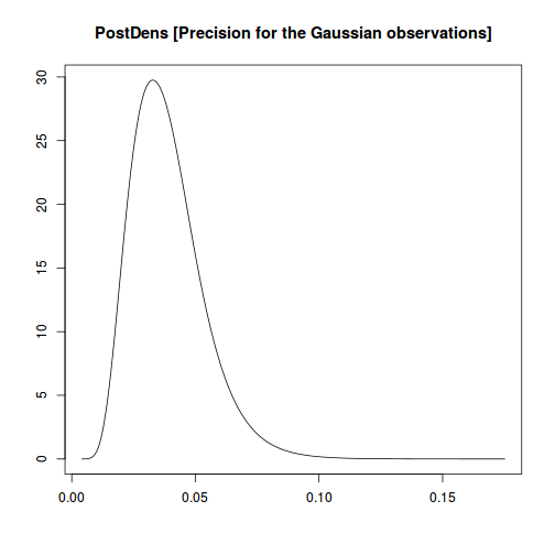
data.inla$summary.hyperpar
                                              mean         sd 0.025quant   0.5quant 0.975quant       mode
Precision for the Gaussian observations 0.03882442 0.01458731 0.01670641 0.03679713 0.07303003 0.03278234
s <- inla.contrib.sd(data.inla, nsamples = 1000)
s$hyper
                                     mean        sd     2.5%    97.5%
sd for the Gaussian observations 5.393922 0.9865159 3.717143 7.535196
5.394 which is similar to the JAGS estimate.
Predictions
There are two main ways to generate predictions in INLA:
- append additional data cases with missing (NA) response to the model input data. Missing response data will not contribute to the likelihood, yet will
be imputed (estimated/predicted given the model trends). In order to illustrate producing a summary plot, I will predict the response for a sequence of predictor
values.
newdata <- data.frame(x=seq(min(data$x, na.rm=TRUE), max(data$x, na.rm=TRUE), len=100), y=NA)
data.pred <- rbind(data, newdata)
#fit the model
data.inla1 <- inla(y~x, data=data.pred, control.compute=list(dic=TRUE, cpo=TRUE, waic=TRUE),
control.predictor=list(compute=TRUE))
#examine the regular summary - not there are no changes to the first fit
summary(data.inla1)
Call:
c("inla(formula = y ~ x, data = data.pred, control.compute = list(dic = TRUE, ",  "    cpo = TRUE, waic = TRUE), control.predictor = list(compute = TRUE))" )

Time used:
 Pre-processing    Running inla Post-processing           Total
         0.0663          0.0489          0.0239          0.1391

Fixed effects:
               mean     sd 0.025quant 0.5quant 0.975quant    mode kld
(Intercept) 40.7441 2.5688    35.6573  40.7440    45.8219 40.7442   0
x           -1.5339 0.2657    -2.0599  -1.5339    -1.0087 -1.5339   0

The model has no random effects

Model hyperparameters:
                                          mean     sd 0.025quant 0.5quant 0.975quant   mode
Precision for the Gaussian observations 0.0438 0.0155     0.0199   0.0418     0.0798 0.0378

Expected number of effective parameters(std dev): 2.00(0.00)
Number of equivalent replicates : 8.00

Deviance Information Criterion (DIC) ...: 100.64
Effective number of parameters .........: 2.634

Watanabe-Akaike information criterion (WAIC) ...: 101.40
Effective number of parameters .................: 2.942

Marginal log-Likelihood:  -64.55
CPO and PIT are computed

Posterior marginals for linear predictor and fitted values computed
#extract the predictor values associated with the appended data newdata <- cbind(newdata, data.inla1$summary.linear.predictor[(nrow(data)+1):nrow(data.pred),]) head(newdata)
                     x  y     mean       sd 0.025quant 0.5quant 0.975quant     mode          kld
predictor.017 1.000000 NA 39.21085 2.339342   34.58500 39.21057   43.83805 39.21031 1.031930e-07
predictor.018 1.151515 NA 38.97844 2.305138   34.42022 38.97816   43.53798 38.97790 1.031943e-07
predictor.019 1.303030 NA 38.74603 2.271133   34.25505 38.74575   43.23831 38.74550 1.031957e-07
predictor.020 1.454545 NA 38.51362 2.237335   34.08947 38.51334   42.93905 38.51309 1.031972e-07
predictor.021 1.606061 NA 38.28120 2.203755   33.92346 38.28094   42.64021 38.28069 1.031987e-07
predictor.022 1.757576 NA 38.04879 2.170402   33.75700 38.04853   42.34183 38.04828 1.032003e-07
newdata <- reshape:::rename(newdata, c("0.025quant"="lower", "0.975quant"="upper"))
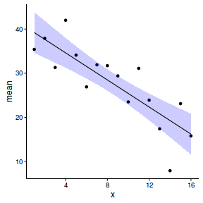
ggplot(newdata, aes(y=mean, x=x)) + geom_point(data=data, aes(y=y)) +
       geom_ribbon(aes(ymin=lower, ymax=upper), fill='blue', alpha=0.2) +
       geom_line() + theme_classic()
- define linear combinations (contrasts) for the predictions. Note, the inla.make.lincombs() function seems a little fragile.
It is vital that it be parsed a data.frame. Furthermore, the model matrix needs to be converted to a data frame using the as.data.frame()
function rather than the data.frame() function as the latter alters the column names and causes problems within INLA.
newdata <- data.frame(x=seq(min(data$x, na.rm=TRUE), max(data$x, na.rm=TRUE), len=100))
Xmat <- model.matrix(~x, data=newdata)
lincomb <- inla.make.lincombs(as.data.frame(Xmat))
#fit the model
data.inla1 <- inla(y~x, lincomb=lincomb,  #include the linear combinations
   data=data,
   control.compute=list(dic=TRUE, cpo=TRUE, waic=TRUE),
   control.inla=list(lincomb.derived.only=FALSE))
#examine the regular summary - not there are no changes to the first fit
#summary(data.inla1)

head(data.inla1$summary.lincomb)
      ID     mean       sd 0.025quant 0.5quant 0.975quant     mode          kld
lc001  1 39.20315 2.359954   34.52673 39.20440   43.86357 39.20635 1.371747e-11
lc002  2 38.97090 2.325452   34.36286 38.97213   43.56320 38.97404 1.372809e-11
lc003  3 38.73864 2.291151   34.19858 38.73985   43.26322 38.74173 1.370907e-11
lc004  4 38.50639 2.257060   34.03389 38.50758   42.96365 38.50942 1.371347e-11
lc005  5 38.27414 2.223188   33.86877 38.27530   42.66452 38.27711 1.373200e-11
lc006  6 38.04188 2.189545   33.70319 38.04303   42.36584 38.04480 1.369481e-11
newdata <- cbind(newdata, data.inla1$summary.lincomb)

newdata <- reshape:::rename(newdata, c("0.025quant"="lower", "0.975quant"="upper"))
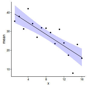
ggplot(newdata, aes(y=mean, x=x)) + geom_point(data=data, aes(y=y)) +
       geom_ribbon(aes(ymin=lower, ymax=upper), fill='blue', alpha=0.2) +
       geom_line() + theme_classic()
One very good way to evaluate the fit of a model is on how well it estimates known parameters. This example generated simulated data given a set of parameters. We could therefore compare the model parameter estimates to these truths.
orig <- data.frame(parameter=factor(c('(Intercept)','x','Sigma2')), value=c(40,-1.5,5))
mod <- subset(data.inla$summary.fixed, select=c('mean','sd','0.025quant','0.975quant'))
mod <- reshape::rename(mod,c("0.025quant"="lower", "0.975quant"="upper"))
colnames(s$hyper) <- c('mean','sd','lower','upper')
mod <- rbind(mod, s$hyper)
mod$parameter <- factor(c('(Intercept)','x','Sigma2'))

ggplot(mod, aes(x=parameter, y=mean)) +
 geom_hline(yintercept=0, linetype='dashed')+
 geom_blank()+
 geom_linerange(aes(x=as.numeric(parameter)-0.05,ymin=lower, ymax=upper)) +
 geom_point(data=orig, aes(y=value, x=as.numeric(factor(parameter))+0.05, fill='Original'), shape=21)+
 geom_point(aes(x=as.numeric(parameter)-0.05, fill='Model'), shape=21)+
 coord_flip()+
 scale_fill_discrete('')+
 scale_y_continuous('')+
 theme_classic()+theme(legend.position=c(1,1), legend.justification=c(1,1))
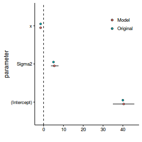
Hence, it appears that the estimated (modelled) parameters are entirely consistent with the original parameters from which the data were simulated.
Multiple linear regression
In the previous example, I displayed many of the basic components of the fitted INLA model. In the remaining examples, we will build upon some of these and ignore others completely - depending on what is required...
Lets say we had set up a natural experiment in which we measured a response ($y$) from each of 20 sampling units ($n=20$) across a landscape. At the same time, we also measured two other continuous covariates ($x1$ and $x2$) from each of the sampling units. As this section is mainly about the generation of artificial data (and not specifically about what to do with the data), understanding the actual details are optional and can be safely skipped. Consequently, I have folded (toggled) this section away.
set.seed(3)
n     = 100
intercept = 5
temp   = runif(n)
nitro = runif(n) + 0.8*temp
int.eff=2
temp.eff <- 0.85
nitro.eff <- 0.5
res = rnorm(n, 0, 1)
coef <- c(int.eff, temp.eff, nitro.eff,int.eff)
mm <- model.matrix(~temp*nitro)

y <- t(coef %*% t(mm)) + res
data <- data.frame(y,x1=temp, x2=nitro, cx1=scale(temp,scale=F), cx2=scale(nitro,scale=F))
$$ y_i = \alpha + \beta_1 x_{1i} + \beta_2 x_{2i} + \varepsilon_i \hspace{4em}\varepsilon_i\sim{}\mathcal{N}(0, \sigma^2) $$
#additive model
summary(lm(y~cx1+cx2, data=data))
Call:
lm(formula = y ~ cx1 + cx2, data = data)

Residuals:
     Min       1Q   Median       3Q      Max
-2.45927 -0.78738 -0.00688  0.71051  2.88492

Coefficients:
            Estimate Std. Error t value Pr(>|t|)
(Intercept)   3.8234     0.1131  33.793  < 2e-16 ***
cx1           3.0250     0.4986   6.067 2.52e-08 ***
cx2           1.3878     0.4281   3.242  0.00163 **
---
Signif. codes:  0 '***' 0.001 '**' 0.01 '*' 0.05 '.' 0.1 ' ' 1

Residual standard error: 1.131 on 97 degrees of freedom
Multiple R-squared:  0.5361,	Adjusted R-squared:  0.5265
F-statistic: 56.05 on 2 and 97 DF,  p-value: < 2.2e-16
confint(lm(y~cx1+cx2, data=data))
                2.5 %   97.5 %
(Intercept) 3.5988464 4.047962
cx1         2.0353869 4.014675
cx2         0.5381745 2.237488
#multiplicative model
summary(lm(y~cx1*cx2, data=data))
Call:
lm(formula = y ~ cx1 * cx2, data = data)

Residuals:
     Min       1Q   Median       3Q      Max
-2.34877 -0.85435  0.06905  0.71265  2.57068

Coefficients:
            Estimate Std. Error t value Pr(>|t|)
(Intercept)   3.6710     0.1315  27.924  < 2e-16 ***
cx1           2.9292     0.4914   5.961 4.15e-08 ***
cx2           1.3445     0.4207   3.196  0.00189 **
cx1:cx2       2.6651     1.2305   2.166  0.03281 *
---
Signif. codes:  0 '***' 0.001 '**' 0.01 '*' 0.05 '.' 0.1 ' ' 1

Residual standard error: 1.111 on 96 degrees of freedom
Multiple R-squared:  0.5577,	Adjusted R-squared:  0.5439
F-statistic: 40.35 on 3 and 96 DF,  p-value: < 2.2e-16
confint(lm(y~cx1*cx2, data=data))
                2.5 %   97.5 %
(Intercept) 3.4100621 3.931972
cx1         1.9537887 3.904642
cx2         0.5094571 2.179451
cx1:cx2     0.2224680 5.107650
#additive model
modelString="
model {
   #Likelihood
   for (i in 1:n) {
      y[i]~dnorm(mu[i],tau)
      mu[i] <- beta0+beta1*x1[i]+beta2*x2[i]
   }
   #Priors
   beta0 ~ dnorm(0.01,1.0E-6)
   beta1 ~ dnorm(0,1.0E-6)
   beta2 ~ dnorm(0,1.0E-6)
   tau <- 1 / (sigma * sigma)
   sigma~dunif(0,100)
 }
"
data.list <- with(data, list(y=y, x1=cx1, x2=cx2, n=nrow(data)))
data.jags <- jags(data=data.list,
           inits=NULL,
           parameters.to.save=c('alpha','beta1', 'beta2', 'sigma'),
           model.file=textConnection(modelString),
           n.chains=3,
           n.iter=100000,
           n.burnin=20000,
                   n.thin=100
           )
Compiling model graph
   Resolving undeclared variables
   Allocating nodes
   Graph Size: 612

Initializing model
print(data.jags)
Inference for Bugs model at "6", fit using jags,
 3 chains, each with 1e+05 iterations (first 20000 discarded), n.thin = 100
 n.sims = 2400 iterations saved
         mu.vect sd.vect    2.5%     25%     50%     75%   97.5%  Rhat n.eff
beta1      3.022   0.504   2.013   2.684   3.006   3.360   4.008 1.001  2400
beta2      1.388   0.435   0.498   1.113   1.403   1.689   2.199 1.001  2400
sigma      1.149   0.082   1.002   1.091   1.144   1.202   1.325 1.000  2400
deviance 309.506   2.931 305.926 307.384 308.842 310.830 317.254 1.001  2400

For each parameter, n.eff is a crude measure of effective sample size,
and Rhat is the potential scale reduction factor (at convergence, Rhat=1).

DIC info (using the rule, pD = var(deviance)/2)
pD = 4.3 and DIC = 313.8
DIC is an estimate of expected predictive error (lower deviance is better).
#multiplicative model
modelString="
model {
   #Likelihood
   for (i in 1:n) {
      y[i]~dnorm(mu[i],tau)
      mu[i] <- beta0+beta1*x1[i]+beta2*x2[i]+beta3*x1[i]*x2[i]
   }
   #Priors
   beta0 ~ dnorm(0.01,1.0E-6)
   beta1 ~ dnorm(0,1.0E-6)
   beta2 ~ dnorm(0,1.0E-6)
   beta3 ~ dnorm(0,1.0E-6)
   tau <- 1 / (sigma * sigma)
   sigma~dunif(0,100)
 }
"
data.list <- with(data, list(y=y, x1=cx1, x2=cx2, n=nrow(data)))
data.jags <- jags(data=data.list,
           inits=NULL,
           parameters.to.save=c('alpha','beta1', 'beta2', 'sigma'),
           model.file=textConnection(modelString),
           n.chains=3,
           n.iter=100000,
           n.burnin=20000,
                   n.thin=100
           )
Compiling model graph
   Resolving undeclared variables
   Allocating nodes
   Graph Size: 713

Initializing model
print(data.jags)
Inference for Bugs model at "7", fit using jags,
 3 chains, each with 1e+05 iterations (first 20000 discarded), n.thin = 100
 n.sims = 2400 iterations saved
         mu.vect sd.vect    2.5%     25%     50%     75%   97.5%  Rhat n.eff
beta1      2.949   0.504   1.971   2.608   2.951   3.284   3.939 1.001  2300
beta2      1.333   0.425   0.484   1.041   1.333   1.618   2.166 1.001  2400
sigma      1.127   0.084   0.977   1.070   1.121   1.181   1.313 1.001  2400
deviance 305.835   3.304 301.533 303.456 305.062 307.486 313.832 1.001  2400

For each parameter, n.eff is a crude measure of effective sample size,
and Rhat is the potential scale reduction factor (at convergence, Rhat=1).

DIC info (using the rule, pD = var(deviance)/2)
pD = 5.5 and DIC = 311.3
DIC is an estimate of expected predictive error (lower deviance is better).
#additive model
data.inla.a <- inla(y~cx1+cx2, data=data, control.compute=list(dic=TRUE, cpo=TRUE, waic=TRUE))
#multiplicative model
data.inla.m <- inla(y~cx1*cx2, data=data, control.compute=list(dic=TRUE, cpo=TRUE, waic=TRUE))
We will first of all explore the INLA summaries for the two models, paying particular attention to the KLD, Expected number of effective parameters and number of equivalent replicates estimates.
summary(data.inla.a)
Call:
c("inla(formula = y ~ cx1 + cx2, data = data, control.compute = list(dic = TRUE, ",  "    cpo = TRUE, waic = TRUE))")

Time used:
 Pre-processing    Running inla Post-processing           Total
         0.0643          0.0534          0.0237          0.1415

Fixed effects:
              mean     sd 0.025quant 0.5quant 0.975quant   mode kld
(Intercept) 3.8234 0.1125     3.6022   3.8234     4.0443 3.8234   0
cx1         3.0245 0.4957     2.0500   3.0245     3.9980 3.0245   0
cx2         1.3880 0.4256     0.5513   1.3880     2.2238 1.3880   0

The model has no random effects

Model hyperparameters:
                                          mean     sd 0.025quant 0.5quant 0.975quant   mode
Precision for the Gaussian observations 0.7968 0.1133     0.5935   0.7905      1.037 0.7797

Expected number of effective parameters(std dev): 3.001(2e-04)
Number of equivalent replicates : 33.32

Deviance Information Criterion (DIC) ...: 312.74
Effective number of parameters .........: 3.647

Watanabe-Akaike information criterion (WAIC) ...: 312.77
Effective number of parameters .................: 3.546

Marginal log-Likelihood:  -173.86
CPO and PIT are computed

Posterior marginals for linear predictor and fitted values computed
summary(data.inla.m)
Call:
c("inla(formula = y ~ cx1 * cx2, data = data, control.compute = list(dic = TRUE, ",  "    cpo = TRUE, waic = TRUE))")

Time used:
 Pre-processing    Running inla Post-processing           Total
         0.0658          0.0525          0.0239          0.1423

Fixed effects:
              mean     sd 0.025quant 0.5quant 0.975quant   mode kld
(Intercept) 3.6712 0.1307     3.4143   3.6712     3.9279 3.6712   0
cx1         2.9288 0.4884     1.9685   2.9288     3.8882 2.9288   0
cx2         1.3446 0.4181     0.5226   1.3446     2.1659 1.3446   0
cx1:cx2     2.6613 1.2224     0.2579   2.6613     5.0621 2.6613   0

The model has no random effects

Model hyperparameters:
                                          mean     sd 0.025quant 0.5quant 0.975quant   mode
Precision for the Gaussian observations 0.8273 0.1182     0.6153   0.8208      1.078 0.8094

Expected number of effective parameters(std dev): 3.999(4e-04)
Number of equivalent replicates : 25.00

Deviance Information Criterion (DIC) ...: 309.98
Effective number of parameters .........: 4.648

Watanabe-Akaike information criterion (WAIC) ...: 309.77
Effective number of parameters .................: 4.227

Marginal log-Likelihood:  -174.76
CPO and PIT are computed

Posterior marginals for linear predictor and fitted values computed
KLD values for all parameters for both models are 0, and thus the Simplified Laplace Approximation is appropriate. The number of effective parameters for both models is approximately 3. Not surprisingly, the additive model therefore has more equivalent replicates per parameter than the multiplicative model. In either case, there appears to be ample replicates per parameter to ensure reliable parameter estimation.
The multiplicative model has evidence of an interaction (95% credibility interval for the interaction parameter do not overlap zero) and both DIC and WAIC values are lower for the multiplicative model than the additive model. Consequently, the multiplicative model would be considered the better of the two models.
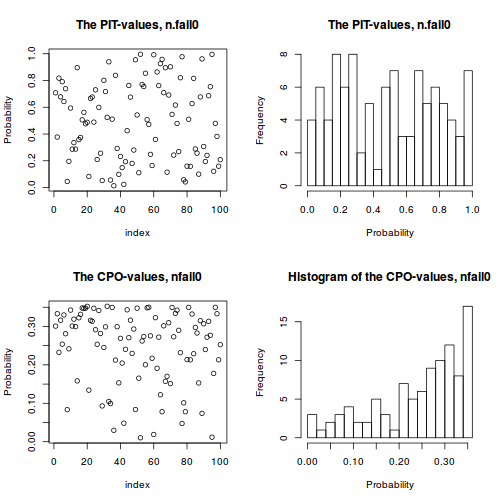
We will examine CPO and PIT from both models.
sum(data.inla.a$cpo$cpo)
[1] 24.45695
-mean(log(data.inla.a$cpo$cpo))
[1] 1.563885
plot(data.inla.a, plot.fixed.effects=FALSE, plot.lincomb=FALSE, plot.random.effects=FALSE,
     plot.hyperparameters=FALSE, plot.predictor=FALSE, plot.q=FALSE, plot.cpo=TRUE,
     single=FALSE)
sum(data.inla.m$cpo$cpo)
[1] 24.4262
-mean(log(data.inla.m$cpo$cpo))
[1] 1.54899
plot(data.inla.m, plot.fixed.effects=FALSE, plot.lincomb=FALSE, plot.random.effects=FALSE,
     plot.hyperparameters=FALSE, plot.predictor=FALSE, plot.q=FALSE, plot.cpo=TRUE,
     single=FALSE)
Predictions
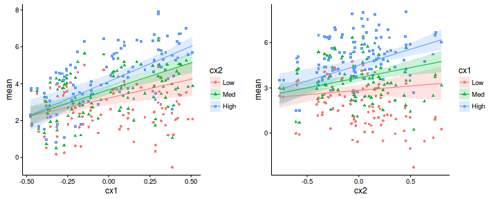
Lets produce partial (conditional) plots for each of the main effects, at a couple of levels of the other covariates (since there was evidence of an interaction). I will do this via the imputation method, however, it could equally be performed via the linear combinations method.
#partial effect of cx1
newdata1 <- expand.grid(cx1=seq(min(data$cx1, na.rm=TRUE), max(data$cx1, na.rm=TRUE), len=100),
                        cx2=c(mean(data$cx2, na.rm=TRUE)-sd(data$cx2, na.rm=TRUE),
                              mean(data$cx2, na.rm=TRUE),
                              mean(data$cx2, na.rm=TRUE)+sd(data$cx2, na.rm=TRUE)),
                        y=NA)

#partial residuals of cx1
newdata1r <- expand.grid(cx1=data$cx1,
                         cx2=c(mean(data$cx2, na.rm=TRUE)-sd(data$cx2, na.rm=TRUE),
                               mean(data$cx2, na.rm=TRUE),
                               mean(data$cx2, na.rm=TRUE)+sd(data$cx2, na.rm=TRUE)),
                         y=NA)

#partial effect of cx2
newdata2 <- expand.grid(cx2=seq(min(data$cx2, na.rm=TRUE), max(data$cx2, na.rm=TRUE), len=100),
                        cx1=c(mean(data$cx1, na.rm=TRUE)-sd(data$cx1, na.rm=TRUE),
                              mean(data$cx1, na.rm=TRUE),
                              mean(data$cx1, na.rm=TRUE)+sd(data$cx1, na.rm=TRUE)),
                        y=NA)

#partial residuals of cx2
newdata2r <- expand.grid(cx2=data$cx2,
                         cx1=c(mean(data$cx1, na.rm=TRUE)-sd(data$cx1, na.rm=TRUE),
                               mean(data$cx1, na.rm=TRUE),
                               mean(data$cx1, na.rm=TRUE)+sd(data$cx1, na.rm=TRUE)),
                         y=NA)

newdata <- rbind(data.frame(Pred='cx1', newdata1),data.frame(Pred='cx2', newdata2),
                 data.frame(Pred='cx1r', newdata1r),data.frame(Pred='cx2r', newdata2r))
data.pred <- rbind(data.frame(Pred='Orig',subset(data, select=c(cx1,cx2,y))), newdata)
#fit the model
data.inla.m1 <- inla(y~cx1*cx2, data=data.pred, control.compute=list(dic=TRUE, cpo=TRUE, waic=TRUE),
                     control.predictor=list(compute=TRUE))

#extract the predictor values associated with the appended data
newdata <- cbind(newdata, data.inla.m1$summary.linear.predictor[(nrow(data)+1):nrow(data.pred),])
newdata <- reshape:::rename(newdata, c("0.025quant"="lower", "0.975quant"="upper"))
newdata1 <- droplevels(subset(newdata, Pred=='cx1'))
newdata1$Cov <- factor(newdata1$cx2, labels=c('Low','Med','High'))
newdata2 <- droplevels(subset(newdata, Pred=='cx2'))
newdata2$Cov <- factor(newdata2$cx1, labels=c('Low','Med','High'))

newdata1r <- droplevels(subset(newdata, Pred=='cx1r'))
newdata1r$Cov <- factor(newdata1$cx2, labels=c('Low','Med','High'))
newdata1r$y <- newdata1r$mean + (newdata1r$mean-data$y)
newdata2r <- droplevels(subset(newdata, Pred=='cx2r'))
newdata2r$Cov <- factor(newdata2$cx1, labels=c('Low','Med','High'))
newdata2r$y <- newdata2r$mean + (newdata2r$mean-data$y)

g1<-ggplot(newdata1, aes(y=mean, x=cx1, shape=Cov,fill=Cov, color=Cov)) +
       geom_point(data=newdata1r, aes(y=y)) +
       geom_ribbon(aes(ymin=lower, ymax=upper), alpha=0.2, color=NA) +
           scale_fill_discrete('cx2')+scale_color_discrete('cx2')+scale_shape_discrete('cx2')+
       geom_line() + theme_classic()
g2<-ggplot(newdata2, aes(y=mean, x=cx2, shape=Cov,fill=Cov, color=Cov)) +
       geom_point(data=newdata2r, aes(y=y)) +
       geom_ribbon(aes(ymin=lower, ymax=upper), alpha=0.2, color=NA) +
           scale_fill_discrete('cx1')+scale_color_discrete('cx1')+scale_shape_discrete('cx1')+
       geom_line() + theme_classic()
library(gridExtra)
grid.arrange(g1,g2, nrow=1)
Single factor ANOVA
Imagine we has designed an experiment in which we had measured the response ($y$) under five different treatments ($x$), each replicated 10 times ($n=10$). As this section is mainly about the generation of artificial data (and not specifically about what to do with the data), understanding the actual details are optional and can be safely skipped. Consequently, I have folded (toggled) this section away.
- the sample size per treatment=10
- the categorical $x$ variable with 5 levels
- the population means associated with the 5 treatment levels are 40, 45, 55, 40, 35 ($\alpha_1=40$, $\alpha_2=45$, $\alpha_3=55$, $\alpha_4=40$, $\alpha_5=30$)
- the data are drawn from normal distributions with a mean of 0 and standard deviation of 3 ($\sigma^2=9$)
set.seed(1)
ngroups <- 5 #number of populations
nsample <- 10 #number of reps in each
pop.means <- c(40, 45, 55, 40, 30) #population mean length
sigma <- 3 #residual standard deviation
n <- ngroups * nsample #total sample size
eps <- rnorm(n, 0, sigma) #residuals
x <- gl(ngroups, nsample, n, lab=LETTERS[1:5]) #factor
means <- rep(pop.means, rep(nsample, ngroups))
X <- model.matrix(~x-1) #create a design matrix
y <- as.numeric(X %*% pop.means+eps)
data <- data.frame(y,x)
head(data)  #print out the first six rows of the data set
         y x
1 38.12064 A
2 40.55093 A
3 37.49311 A
4 44.78584 A
5 40.98852 A
6 37.53859 A
$$ y_i = \alpha + \beta X_{i} + \varepsilon_i \hspace{4em}\varepsilon_i\sim{}\mathcal{N}(0, \sigma^2) $$
data.lm <- lm(y~x, data=data)
summary(data.lm)
Call:
lm(formula = y ~ x, data = data)

Residuals:
    Min      1Q  Median      3Q     Max
-7.3906 -1.2752  0.3278  1.7931  4.3892

Coefficients:
            Estimate Std. Error t value Pr(>|t|)
(Intercept) 40.39661    0.81333  49.668  < 2e-16 ***
xB           5.34993    1.15023   4.651 2.91e-05 ***
xC          14.20237    1.15023  12.347 4.74e-16 ***
xD          -0.03442    1.15023  -0.030    0.976
xE          -9.99420    1.15023  -8.689 3.50e-11 ***
---
Signif. codes:  0 '***' 0.001 '**' 0.01 '*' 0.05 '.' 0.1 ' ' 1

Residual standard error: 2.572 on 45 degrees of freedom
Multiple R-squared:  0.9129,	Adjusted R-squared:  0.9052
F-statistic: 117.9 on 4 and 45 DF,  p-value: < 2.2e-16
modelString="
model {
   #Likelihood
   for (i in 1:n) {
      y[i]~dnorm(mean[i],tau)
      mean[i] <- inprod(beta[],X[i,])
   }
   #Priors
   for (i in 1:ngroups) {
     beta[i] ~ dnorm(0, 1.0E-6)
   }
   sigma ~ dunif(0, 100)
   tau <- 1 / (sigma * sigma)


   #Contrasts
   Group.means[1] <- beta[1]
   for (i in 2:ngroups) {
     Group.means[i] <- beta[i]+beta[1]
   }

   #Pairwise effects
   for (i in 1:ngroups) {
     for (j in 1:ngroups) {
	   eff[i,j] <- Group.means[i] - Group.means[j]
	 }
   }

   #Specific comparisons
   Comp1 <- Group.means[3] - Group.means[5]
   Comp2 <- (Group.means[1] + Group.means[2])/2 -
            (Group.means[3] + Group.means[4] + Group.means[5])/3
 }
"
X <- model.matrix(~x, data)
data.list <- with(data,
        list(y=y,
                 X=X,
         n=nrow(data),
         ngroups=ncol(X)
         )
)
data.jags <- jags(data=data.list,
          inits=NULL,
          parameters.to.save=c('beta','sigma', 'eff', 'Comp1', 'Comp2'),
          model.file=textConnection(modelString),
          n.chains=3,
          n.iter=10000,
          n.burnin=2000,
      n.thin=100
          )
Compiling model graph
   Resolving undeclared variables
   Allocating nodes
   Graph Size: 406

Initializing model
print(data.jags)
Inference for Bugs model at "6", fit using jags,
 3 chains, each with 10000 iterations (first 2000 discarded), n.thin = 100
 n.sims = 240 iterations saved
         mu.vect sd.vect    2.5%     25%     50%     75%   97.5%  Rhat n.eff
Comp1     24.082   1.190  21.973  23.314  24.100  24.837  26.545 1.006   210
Comp2      1.310   0.798  -0.236   0.771   1.382   1.809   2.765 1.001   240
beta[1]   40.440   0.844  38.720  39.847  40.472  40.974  42.135 1.011   140
beta[2]    5.326   1.222   2.887   4.578   5.278   6.102   7.821 1.021   120
beta[3]   14.133   1.224  11.678  13.358  14.106  14.953  16.338 0.999   240
beta[4]   -0.124   1.155  -2.139  -0.883  -0.121   0.614   2.279 1.031   120
beta[5]   -9.949   1.142 -11.916 -10.737  -9.991  -9.144  -7.772 1.005   240
eff[1,1]   0.000   0.000   0.000   0.000   0.000   0.000   0.000 1.000     1
eff[2,1]   5.326   1.222   2.887   4.578   5.278   6.102   7.821 1.021   120
eff[3,1]  14.133   1.224  11.678  13.358  14.106  14.953  16.338 0.999   240
eff[4,1]  -0.124   1.155  -2.139  -0.883  -0.121   0.614   2.279 1.031   120
eff[5,1]  -9.949   1.142 -11.916 -10.737  -9.991  -9.144  -7.772 1.005   240
eff[1,2]  -5.326   1.222  -7.821  -6.102  -5.278  -4.578  -2.887 1.010   140
eff[2,2]   0.000   0.000   0.000   0.000   0.000   0.000   0.000 1.000     1
eff[3,2]   8.806   1.343   6.244   7.881   8.764   9.745  11.556 1.024   140
eff[4,2]  -5.450   1.215  -7.740  -6.381  -5.380  -4.673  -3.025 0.996   240
eff[5,2] -15.276   1.222 -17.554 -15.996 -15.369 -14.446 -12.564 0.996   240
eff[1,3] -14.133   1.224 -16.338 -14.953 -14.106 -13.358 -11.678 0.999   240
eff[2,3]  -8.806   1.343 -11.556  -9.745  -8.764  -7.881  -6.244 1.016   140
eff[3,3]   0.000   0.000   0.000   0.000   0.000   0.000   0.000 1.000     1
eff[4,3] -14.257   1.168 -16.241 -15.121 -14.245 -13.474 -11.660 1.018    98
eff[5,3] -24.082   1.190 -26.545 -24.837 -24.100 -23.314 -21.973 1.006   210
eff[1,4]   0.124   1.155  -2.279  -0.614   0.121   0.883   2.139 1.031   120
eff[2,4]   5.450   1.215   3.025   4.673   5.380   6.381   7.740 0.996   240
eff[3,4]  14.257   1.168  11.660  13.474  14.245  15.121  16.241 1.020    94
eff[4,4]   0.000   0.000   0.000   0.000   0.000   0.000   0.000 1.000     1
eff[5,4]  -9.825   1.220 -12.114 -10.643  -9.854  -8.901  -7.713 1.001   240
eff[1,5]   9.949   1.142   7.772   9.144   9.991  10.737  11.916 1.005   240
eff[2,5]  15.276   1.222  12.564  14.446  15.369  15.996  17.554 0.996   240
eff[3,5]  24.082   1.190  21.973  23.314  24.100  24.837  26.545 1.006   210
eff[4,5]   9.825   1.220   7.713   8.901   9.854  10.643  12.114 0.999   240
eff[5,5]   0.000   0.000   0.000   0.000   0.000   0.000   0.000 1.000     1
sigma      2.655   0.298   2.153   2.462   2.622   2.823   3.228 0.998   240
deviance 237.918   3.727 232.555 235.288 237.245 239.878 246.813 1.010   170

For each parameter, n.eff is a crude measure of effective sample size,
and Rhat is the potential scale reduction factor (at convergence, Rhat=1).

DIC info (using the rule, pD = var(deviance)/2)
pD = 6.9 and DIC = 244.8
DIC is an estimate of expected predictive error (lower deviance is better).
In preparation for fitting this model, we will also consider a number of contrasts (as we did for the Bayesian (JAGS) version of the analysis. Firstly, we will append missing response data in order to generate cell means predictions (for the summary plot) and secondly, we will define linear combinations (contrasts) to provide the pairwise and planned comparisons.
newdata <- data.frame(x=levels(data$x), y=NA)
data.pred <- rbind(data,  newdata)
#Define linear combinations (pairwise comparisons)
library(multcomp)
tuk.mat <- contrMat(n=table(newdata$x), type="Tukey")
Xmat <- model.matrix(~x, data=newdata)
pairwise.Xmat <- tuk.mat %*% Xmat
pairwise.Xmat
      (Intercept) xB xC xD xE
B - A           0  1  0  0  0
C - A           0  0  1  0  0
D - A           0  0  0  1  0
E - A           0  0  0  0  1
C - B           0 -1  1  0  0
D - B           0 -1  0  1  0
E - B           0 -1  0  0  1
D - C           0  0 -1  1  0
E - C           0  0 -1  0  1
E - D           0  0  0 -1  1
#Define linear combinations (planned contrasts)
comp.Xmat <- rbind(Comp1=c(0,0,1,0,-1), Comp2=c(1/2,1/2,-1/3,-1/3,-1/3))
#make these appropriate for the treatment contrasts applied in the model fit
comp.Xmat <-cbind(0,comp.Xmat %*% contr.treatment(5))
rownames(comp.Xmat) <- c("Grp 3 vs 5","Grp 1,2 vs 3,4,5")

Xmat <- rbind(pairwise.Xmat, comp.Xmat)
Xmat
                 (Intercept)   xB         xC         xD         xE
B - A                      0  1.0  0.0000000  0.0000000  0.0000000
C - A                      0  0.0  1.0000000  0.0000000  0.0000000
D - A                      0  0.0  0.0000000  1.0000000  0.0000000
E - A                      0  0.0  0.0000000  0.0000000  1.0000000
C - B                      0 -1.0  1.0000000  0.0000000  0.0000000
D - B                      0 -1.0  0.0000000  1.0000000  0.0000000
E - B                      0 -1.0  0.0000000  0.0000000  1.0000000
D - C                      0  0.0 -1.0000000  1.0000000  0.0000000
E - C                      0  0.0 -1.0000000  0.0000000  1.0000000
E - D                      0  0.0  0.0000000 -1.0000000  1.0000000
Grp 3 vs 5                 0  0.0  1.0000000  0.0000000 -1.0000000
Grp 1,2 vs 3,4,5           0  0.5 -0.3333333 -0.3333333 -0.3333333
lincomb <- inla.make.lincombs(as.data.frame(Xmat))
Now lets fit the model.
#fit the model
data.inla1 <- inla(y~x, lincomb=lincomb,  #include the linear combinations
   data=data.pred,
   control.compute=list(dic=TRUE, cpo=TRUE, waic=TRUE),
   control.inla=list(lincomb.derived.only=TRUE))
#examine the regular summary - not there are no changes to the first fit
summary(data.inla1)
Call:
c("inla(formula = y ~ x, data = data.pred, lincomb = lincomb, control.compute = list(dic = TRUE, ",  "    cpo = TRUE, waic = TRUE), control.inla = list(lincomb.derived.only = TRUE))" )

Time used:
 Pre-processing    Running inla Post-processing           Total
         0.1363          0.0730          0.0552          0.2646

Fixed effects:
               mean     sd 0.025quant 0.5quant 0.975quant    mode kld
(Intercept) 40.4027 0.8021    38.8235  40.4026    41.9806 40.4025   0
xB           5.3404 1.1346     3.1059   5.3405     7.5715  5.3407   0
xC          14.1871 1.1346    11.9524  14.1873    16.4180 14.1877   0
xD          -0.0405 1.1346    -2.2748  -0.0405     2.1908 -0.0403   0
xE          -9.9939 1.1346   -12.2279  -9.9939    -7.7624 -9.9939   0

Linear combinations (derived):
     ID     mean     sd 0.025quant 0.5quant 0.975quant     mode kld
lc01  1   5.3404 1.1346     3.1059   5.3405     7.5715   5.3407   0
lc02  2  14.1871 1.1346    11.9524  14.1873    16.4180  14.1877   0
lc03  3  -0.0405 1.1346    -2.2748  -0.0405     2.1908  -0.0403   0
lc04  4  -9.9939 1.1346   -12.2279  -9.9939    -7.7624  -9.9939   0
lc05  5   8.8467 1.1355     6.6106   8.8468    11.0799   8.8470   0
lc06  6  -5.3809 1.1355    -7.6166  -5.3810    -3.1474  -5.3810   0
lc07  7 -15.3342 1.1355   -17.5697 -15.3344   -13.1005 -15.3346   0
lc08  8 -14.2276 1.1355   -16.4632 -14.2278   -11.9939 -14.2280   0
lc09  9 -24.1810 1.1355   -26.4163 -24.1812   -21.9471 -24.1816   0
lc10 10  -9.9534 1.1355   -12.1890  -9.9535    -7.7198  -9.9536   0
lc11 11  24.1810 1.1355    21.9444  24.1812    26.4138  24.1816   0
lc12 12   1.2859 0.7326    -0.1565   1.2859     2.7269   1.2859   0

The model has no random effects

Model hyperparameters:
                                          mean     sd 0.025quant 0.5quant 0.975quant   mode
Precision for the Gaussian observations 0.1577 0.0325     0.1018   0.1551      0.229 0.1506

Expected number of effective parameters(std dev): 4.995(9e-04)
Number of equivalent replicates : 10.01

Deviance Information Criterion (DIC) ...: 242.49
Effective number of parameters .........: 5.651

Watanabe-Akaike information criterion (WAIC) ...: 243.15
Effective number of parameters .................: 5.727

Marginal log-Likelihood:  -142.21
CPO and PIT are computed

Posterior marginals for linear predictor and fitted values computed
Parameter estimates are entirely consistent with the Frequentist and JAGS outcomes. Lets explore the various contrasts. These are captured in the summary.lincomb.derived element of the INLA list. To make this a little more informative (so we can see what each contrast represents, I will apply the rownames from the Xmat.
rownames(data.inla1$summary.lincomb.derived) <- rownames(Xmat)
data.inla1$summary.lincomb.derived
                 ID         mean        sd  0.025quant     0.5quant 0.975quant         mode kld
B - A             1   5.34035821 1.1345555   3.1059307   5.34045527   7.571501   5.34073924   0
C - A             2  14.18709661 1.1345572  11.9524362  14.18727158  16.418038  14.18770537   0
D - A             3  -0.04051494 1.1345548  -2.2748016  -0.04046525   2.190752  -0.04027242   0
E - A             4  -9.99387467 1.1345544 -12.2279022  -9.99391263  -7.762378  -9.99388837   0
C - B             5   8.84673840 1.1354933   6.6105973   8.84678312  11.079883   8.84696648   0
D - B             6  -5.38087314 1.1354931  -7.6166440  -5.38095391  -3.147399  -5.38101187   0
E - B             7 -15.33423287 1.1354941 -17.5697471 -15.33440142 -13.100526 -15.33462821   0
D - C             8 -14.22761155 1.1354940 -16.4631542 -14.22777033 -11.993931 -14.22797835   0
E - C             9 -24.18097128 1.1354959 -26.4162589 -24.18121785 -21.947056 -24.18159469   0
E - D            10  -9.95335973 1.1354934 -12.1890125  -9.95348082  -7.719779  -9.95361634   0
Grp 3 vs 5       11  24.18097128 1.1354959  21.9444267  24.18115124  26.413765  24.18159469   0
Grp 1,2 vs 3,4,5 12   1.28594339 0.7325942  -0.1565176   1.28589156   2.726922   1.28585466   0
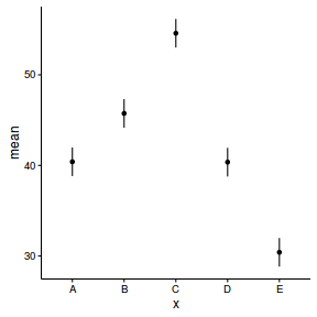
Finally, it is time to extract the predicted values from the linear predictor and plot the cell means.
#summary figure
newdata <- cbind(newdata, data.inla1$summary.linear.predictor[(nrow(data)+1):nrow(data.pred),])
newdata <- reshape:::rename(newdata, c("0.025quant"="lower", "0.975quant"="upper"))

ggplot(newdata, aes(y=mean, x=x)) + geom_linerange(aes(ymin=lower, ymax=upper))+
       geom_point() + theme_classic()
Factorial ANOVA
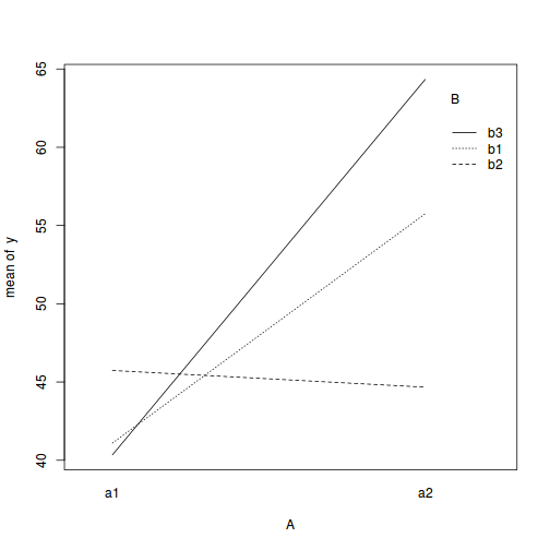
Imagine we has designed an experiment in which we had measured the response ($y$) under a combination of two different potential influences (Factor A: levels $a1$ and $a2$; and Factor B: levels $b1$, $b2$ and $b3$), each combination replicated 10 times ($n=10$). As this section is mainly about the generation of artificial data (and not specifically about what to do with the data), understanding the actual details are optional and can be safely skipped. Consequently, I have folded (toggled) this section away.
- the sample size per treatment=10
- factor A with 2 levels
- factor B with 3 levels
- the 6 effects parameters are 40, 15, 5, 0, -15,10 ($\mu_{a1b1}=40$, $\mu_{a2b1}=40+15=55$, $\mu_{a1b2}=40+5=45$, $\mu_{a1b3}=40+0=40$, $\mu_{a2b2}=40+15+5-15=45$ and $\mu_{a2b3}=40+15+0+10=65$)
- the data are drawn from normal distributions with a mean of 0 and standard deviation of 3 ($\sigma^2=9$)
set.seed(1)
nA <- 2 #number of levels of A
nB <- 3 #number of levels of B
nsample <- 10 #number of reps in each
A <- gl(nA,1,nA, lab=paste("a",1:nA,sep=""))
B <- gl(nB,1,nB, lab=paste("b",1:nB,sep=""))
data <-expand.grid(A=A,B=B, n=1:nsample)
X <- model.matrix(~A*B, data=data)
eff <- c(40,15,5,0,-15,10)
sigma <- 3 #residual standard deviation
n <- nrow(data)
eps <- rnorm(n, 0, sigma) #residuals
data$y <- as.numeric(X %*% eff+eps)
head(data)  #print out the first six rows of the data set
   A  B n        y
1 a1 b1 1 38.12064
2 a2 b1 1 55.55093
3 a1 b2 1 42.49311
4 a2 b2 1 49.78584
5 a1 b3 1 40.98852
6 a2 b3 1 62.53859
with(data,interaction.plot(A,B,y))
## ALTERNATIVELY, we could supply the population means
## and get the effect parameters from these.
## To correspond to the model matrix, enter the population
## means in the order of:
## a1b1, a2b1, a1b1, a2b2,a1b3,a2b3
pop.means <- as.matrix(c(40,55,45,45,40,65),byrow=F)
## Generate a minimum model matrix for the effects
XX <-model.matrix(~A*B, expand.grid(A=factor(1:2),B=factor(1:3)))
## Use the solve() function to solve what are effectively simultaneous equations
(eff<-as.vector(solve(XX,pop.means)))
[1] 40 15 5 0 -15 10
data$y <- as.numeric(X %*% eff+eps)
$$ y_i = \alpha + \beta X_{i} + \varepsilon_i \hspace{4em}\varepsilon_i\sim{}\mathcal{N}(0, \sigma^2) $$
data.lm <- lm(y~A*B, data=data)
summary(data.lm)
Call:
lm(formula = y ~ A * B, data = data)

Residuals:
    Min      1Q  Median      3Q     Max
-7.3944 -1.5753  0.2281  1.5575  5.1909

Coefficients:
            Estimate Std. Error t value Pr(>|t|)
(Intercept)  41.0988     0.8218  50.010  < 2e-16 ***
Aa2          14.6515     1.1622  12.606  < 2e-16 ***
Bb2           4.6386     1.1622   3.991   0.0002 ***
Bb3          -0.7522     1.1622  -0.647   0.5202
Aa2:Bb2     -15.7183     1.6436  -9.563 3.24e-13 ***
Aa2:Bb3       9.3352     1.6436   5.680 5.54e-07 ***
---
Signif. codes:  0 '***' 0.001 '**' 0.01 '*' 0.05 '.' 0.1 ' ' 1

Residual standard error: 2.599 on 54 degrees of freedom
Multiple R-squared:  0.9245,	Adjusted R-squared:  0.9175
F-statistic: 132.3 on 5 and 54 DF,  p-value: < 2.2e-16
modelString="
model {
   #Likelihood
   for (i in 1:n) {
      y[i]~dnorm(mean[i],tau)
      mean[i] <- inprod(beta[],X[i,])
   }
   #Priors and derivatives
   for (i in 1:p) {
     beta[i] ~ dnorm(0, 1.0E-6) #prior
   }
   sigma ~ dunif(0, 100)
   tau <- 1 / (sigma * sigma)
 }
"
X <- model.matrix(~A*B, data)
data.list <- with(data,
                  list(y=y,
                       X=X,
                       n=nrow(data),
                       p=ncol(X)
                       )
)

data.jags <- jags(data=data.list,
          inits=NULL,
          parameters.to.save=c('beta','sigma'),
          model.file=textConnection(modelString),
          n.chains=3,
          n.iter=10000,
          n.burnin=2000,
      n.thin=100
          )
Compiling model graph
   Resolving undeclared variables
   Allocating nodes
   Graph Size: 502

Initializing model
print(data.jags)
Inference for Bugs model at "8", fit using jags,
 3 chains, each with 10000 iterations (first 2000 discarded), n.thin = 100
 n.sims = 240 iterations saved
         mu.vect sd.vect    2.5%     25%     50%     75%   97.5%  Rhat n.eff
beta[1]   40.999   0.894  39.444  40.348  40.972  41.622  42.780 1.005   240
beta[2]   14.849   1.136  12.625  14.026  14.859  15.554  16.912 0.997   240
beta[3]    4.793   1.204   2.600   4.029   4.806   5.659   6.884 1.012   240
beta[4]   -0.646   1.214  -3.104  -1.375  -0.585   0.182   1.544 0.996   240
beta[5]  -16.021   1.739 -19.540 -16.976 -15.918 -14.945 -12.609 0.996   240
beta[6]    9.216   1.565   6.271   8.162   9.269  10.179  12.699 1.002   240
sigma      2.665   0.281   2.238   2.446   2.650   2.837   3.309 1.000   240
deviance 286.159   3.935 280.494 283.270 285.659 288.017 293.962 1.017   210

For each parameter, n.eff is a crude measure of effective sample size,
and Rhat is the potential scale reduction factor (at convergence, Rhat=1).

DIC info (using the rule, pD = var(deviance)/2)
pD = 7.7 and DIC = 293.9
DIC is an estimate of expected predictive error (lower deviance is better).
newdata <- expand.grid(A=levels(data$A), B=levels(data$B), y=NA)
data.pred <- rbind(subset(data, select=c(A,B,y)),  newdata)
In addition to fitting the model in INLA, it might be useful to also derive the marginal effects of one of the factors (A) at each level of the other factor (B).
#Define linear combinations (planned contrasts)
Xmat <- model.matrix(~A*B, data=newdata)
cbind(newdata, Xmat)
   A  B  y (Intercept) Aa2 Bb2 Bb3 Aa2:Bb2 Aa2:Bb3
1 a1 b1 NA           1   0   0   0       0       0
2 a2 b1 NA           1   1   0   0       0       0
3 a1 b2 NA           1   0   1   0       0       0
4 a2 b2 NA           1   1   1   0       1       0
5 a1 b3 NA           1   0   0   1       0       0
6 a2 b3 NA           1   1   0   1       0       1
library(plyr)
Xmat <- daply(cbind(newdata, Xmat), ~B, function(x) {
    x[2,] - x[1,]
})
Xmat
B    A  B  y  (Intercept) Aa2 Bb2 Bb3 Aa2:Bb2 Aa2:Bb3
  b1 NA NA NA 0           1   0   0   0       0
  b2 NA NA NA 0           1   0   0   1       0
  b3 NA NA NA 0           1   0   0   0       1
lincomb <- inla.make.lincombs(as.data.frame(Xmat[,-1:-3]))
Now lets fit the model.
#fit the model
data.inla <- inla(y~A*B,
   data=data.pred,
   lincomb=lincomb,
   control.compute=list(dic=TRUE, cpo=TRUE, waic=TRUE),
   control.inla=list(lincomb.derived.only=TRUE))
#examine the regular summary - not there are no changes to the first fit
summary(data.inla)
Call:
c("inla(formula = y ~ A * B, data = data.pred, lincomb = lincomb, ",  "    control.compute = list(dic = TRUE, cpo = TRUE, waic = TRUE), ",  "    control.inla = list(lincomb.derived.only = TRUE))")

Time used:
 Pre-processing    Running inla Post-processing           Total
         0.0820          0.0597          0.0309          0.1727

Fixed effects:
                mean     sd 0.025quant 0.5quant 0.975quant     mode kld
(Intercept)  41.1152 0.8119    39.5179  41.1150    42.7118  41.1147   0
Aa2          14.6213 1.1474    12.3621  14.6216    16.8761  14.6223   0
Bb2           4.6088 1.1479     2.3485   4.6091     6.8648   4.6098   0
Bb3          -0.7619 1.1479    -3.0216  -0.7619     1.4946  -0.7616   0
Aa2:Bb2     -15.6643 1.6225   -18.8558 -15.6650   -12.4729 -15.6661   0
Aa2:Bb3       9.3525 1.6225     6.1598   9.3523    12.5428   9.3519   0

Linear combinations (derived):
    ID    mean     sd 0.025quant 0.5quant 0.975quant    mode kld
lc1  1 14.6213 1.1474    12.3621  14.6216    16.8761 14.6223   0
lc2  2 -1.0430 1.1491    -3.3039  -1.0434     1.2168 -1.0438   0
lc3  3 23.9738 1.1491    21.7117  23.9739    26.2326 23.9742   0

The model has no random effects

Model hyperparameters:
                                          mean    sd 0.025quant 0.5quant 0.975quant   mode
Precision for the Gaussian observations 0.1534 0.029      0.103   0.1513     0.2164 0.1476

Expected number of effective parameters(std dev): 5.991(0.0014)
Number of equivalent replicates : 10.02

Deviance Information Criterion (DIC) ...: 292.00
Effective number of parameters .........: 6.649

Watanabe-Akaike information criterion (WAIC) ...: 292.64
Effective number of parameters .................: 6.634

Marginal log-Likelihood:  -169.80
CPO and PIT are computed

Posterior marginals for linear predictor and fitted values computed
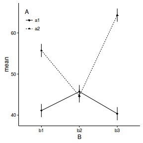
Finally, it is time to extract the predicted values from the linear predictor and plot the cell means.
#summary figure
newdata <- cbind(newdata, data.inla$summary.linear.predictor[(nrow(data)+1):nrow(data.pred),])
newdata <- reshape:::rename(newdata, c("0.025quant"="lower", "0.975quant"="upper"))
head(newdata)
              A  B  y     mean        sd    lower 0.5quant    upper     mode          kld
predictor.61 a1 b1 NA 41.11522 0.8118338 39.52008 41.11503 42.71099 41.11468 1.674684e-09
predictor.62 a2 b1 NA 55.73648 0.8123780 54.13916 55.73664 57.33253 55.73696 1.885519e-09
predictor.63 a1 b2 NA 45.72401 0.8126511 44.12616 45.72417 47.32061 45.72447 1.878400e-09
predictor.64 a2 b2 NA 44.68097 0.8129257 43.08342 44.68085 46.27874 44.68063 1.702529e-09
predictor.65 a1 b3 NA 40.35329 0.8126503 38.75616 40.35321 41.95042 40.35307 1.732000e-09
predictor.66 a2 b3 NA 64.32707 0.8129237 62.72894 64.32714 65.92440 64.32729 1.822437e-09
ggplot(newdata, aes(y=mean, x=B, shape=A)) + geom_linerange(aes(ymin=lower, ymax=upper))+
       geom_point() + geom_line(aes(x=as.numeric(B), linetype=A)) + theme_classic()+
       theme(legend.position=c(0,1),legend.justification=c(0,1))
Logistic regression (binary response)
Lets say we wanted to model the presence/absence of an item ($y$) against a continuous predictor ($x$) As this section is mainly about the generation of artificial data (and not specifically about what to do with the data), understanding the actual details are optional and can be safely skipped. Consequently, I have folded (toggled) this section away.
- the sample size = 20
- the continuous $x$ variable is a random uniform spread of measurements between 1 and 20
- the rate of change in log odds ratio per unit change in x (slope) = 0.5. The magnitude of the slope is an indicator of how abruptly the log odds ratio changes. A very abrupt change would occur if there was very little variability in the trend. That is, a large slope would be indicative of a threshold effect. A lower slope indicates a gradual change in odds ratio and thus a less obvious and precise switch between the likelihood of 1 vs 0.
- the inflection point (point where the slope of the line is greatest) = 10. The inflection point indicates the value of the predictor ($x$) where the log Odds are 50% (switching between 1 being more likely and 0 being more likely). This is also known as the LD50.
- the intercept (which has no real interpretation) is equal to the negative of the slope multiplied by the inflection point
- to generate the values of $y$ expected at each $x$ value, we evaluate the linear predictor. These expected values are then transformed into a scale mapped by (0,1) by using the inverse logit function $\frac{e^{linear~predictor}}{1+e^{linear~predictor}}$
- finally, we generate $y$ values by using the expected $y$ values as probabilities when drawing random numbers from a binomial distribution. This step adds random noise to the expected $y$ values and returns only 1's and 0's.
set.seed(8)
#The number of samples
n.x <- 20
#Create x values that at uniformly distributed throughout the rate of 1 to 20
x <- sort(runif(n = n.x, min = 1, max =20))
#The slope is the rate of change in log odds ratio for each unit change in x
# the smaller the slope, the slower the change (more variability in data too)
slope=0.5
#Inflection point is where the slope of the line is greatest
#this is also the LD50 point
inflect <- 10
#Intercept (no interpretation)
intercept <- -1*(slope*inflect)
#The linear predictor
linpred <- intercept+slope*x
#Predicted y values
y.pred <- exp(linpred)/(1+exp(linpred))
#Add some noise and make binomial
n.y <-rbinom(n=n.x,20,p=0.9)
y<- rbinom(n = n.x,size=1, prob = y.pred)
dat <- data.frame(y,x)
$$ log\left(\frac{\pi}{1-\pi}\right)=\beta_0+\beta_1x_1+\epsilon_i, \hspace{1cm}\epsilon\sim Binom(\lambda) $$
dat.glm <- glm(y~x, data=dat, family="binomial")
summary(dat.glm)
Call:
glm(formula = y ~ x, family = "binomial", data = dat)

Deviance Residuals:
     Min        1Q    Median        3Q       Max
-1.97157  -0.33665  -0.08191   0.30035   1.59628

Coefficients:
            Estimate Std. Error z value Pr(>|z|)
(Intercept)  -6.9899     3.1599  -2.212   0.0270 *
x             0.6559     0.2936   2.234   0.0255 *
---
Signif. codes:  0 '***' 0.001 '**' 0.01 '*' 0.05 '.' 0.1 ' ' 1

(Dispersion parameter for binomial family taken to be 1)

    Null deviance: 27.526  on 19  degrees of freedom
Residual deviance: 11.651  on 18  degrees of freedom
AIC: 15.651

Number of Fisher Scoring iterations: 6
modelString="
model{
  for (i in 1:N) {
    y[i] ~ dbern(p[i])
    logit(p[i]) <- max(-20,min(20,beta0+beta1*x[i]))
  }
  beta0 ~ dnorm(0,1.0E-06)
  beta1 ~ dnorm(0,1.0E-06)
}
"
dat.list <- with(dat, list(y=y, x=x, N=nrow(dat)))
dat.jags <- jags(data=dat.list,model.file=textConnection(modelString),
                   param=c('beta0','beta1'),
                   n.chains=3, n.iter=20000, n.burnin=10000, n.thin=100)
Compiling model graph
   Resolving undeclared variables
   Allocating nodes
   Graph Size: 147

Initializing model
print(dat.jags)
Inference for Bugs model at "9", fit using jags,
 3 chains, each with 20000 iterations (first 10000 discarded), n.thin = 100
 n.sims = 300 iterations saved
         mu.vect sd.vect    2.5%     25%    50%    75%  97.5%  Rhat n.eff
beta0     -9.497   3.970 -18.493 -12.068 -8.922 -6.449 -3.740 1.004   300
beta1      0.898   0.370   0.353   0.612  0.844  1.123  1.772 1.003   300
deviance  13.872   2.108  11.683  12.301 13.291 14.811 19.290 1.018   200

For each parameter, n.eff is a crude measure of effective sample size,
and Rhat is the potential scale reduction factor (at convergence, Rhat=1).

DIC info (using the rule, pD = var(deviance)/2)
pD = 2.2 and DIC = 16.1
DIC is an estimate of expected predictive error (lower deviance is better).
library(rstan)
modelString="
data {
   int<lower=1> n;
   int<lower=1> nX;
   int y[n];
   matrix [n,nX] X;
}
parameters {
   vector [nX] beta;
}
transformed parameters {
   vector [n] mu;
   mu<-X*beta;
}
model {
   beta ~ normal(0,1000);
   y ~ binomial_logit(1, mu);
}
"
Xmat <- model.matrix(~x,data=dat)
dat.list <- with(dat, list(y = y, X = Xmat, nX=ncol(Xmat),n = nrow(dat)))

library(rstan)
dat.rstan <- stan(data=dat.list,
           model_code=modelString,
           chains=3,
           iter=1000,
           warmup=500,
                   thin=2,
           save_dso=TRUE
           )
SAMPLING FOR MODEL '8378cae68bcb88c343bcb3d714aeb387' NOW (CHAIN 1).

Chain 1, Iteration:   1 / 1000 [  0%]  (Warmup)
Chain 1, Iteration: 100 / 1000 [ 10%]  (Warmup)
Chain 1, Iteration: 200 / 1000 [ 20%]  (Warmup)
Chain 1, Iteration: 300 / 1000 [ 30%]  (Warmup)
Chain 1, Iteration: 400 / 1000 [ 40%]  (Warmup)
Chain 1, Iteration: 500 / 1000 [ 50%]  (Warmup)
Chain 1, Iteration: 501 / 1000 [ 50%]  (Sampling)
Chain 1, Iteration: 600 / 1000 [ 60%]  (Sampling)
Chain 1, Iteration: 700 / 1000 [ 70%]  (Sampling)
Chain 1, Iteration: 800 / 1000 [ 80%]  (Sampling)
Chain 1, Iteration: 900 / 1000 [ 90%]  (Sampling)
Chain 1, Iteration: 1000 / 1000 [100%]  (Sampling)#
#  Elapsed Time: 0.060304 seconds (Warm-up)
#                0.053233 seconds (Sampling)
#                0.113537 seconds (Total)
#

SAMPLING FOR MODEL '8378cae68bcb88c343bcb3d714aeb387' NOW (CHAIN 2).

Chain 2, Iteration:   1 / 1000 [  0%]  (Warmup)
Chain 2, Iteration: 100 / 1000 [ 10%]  (Warmup)
Chain 2, Iteration: 200 / 1000 [ 20%]  (Warmup)
Chain 2, Iteration: 300 / 1000 [ 30%]  (Warmup)
Chain 2, Iteration: 400 / 1000 [ 40%]  (Warmup)
Chain 2, Iteration: 500 / 1000 [ 50%]  (Warmup)
Chain 2, Iteration: 501 / 1000 [ 50%]  (Sampling)
Chain 2, Iteration: 600 / 1000 [ 60%]  (Sampling)
Chain 2, Iteration: 700 / 1000 [ 70%]  (Sampling)
Chain 2, Iteration: 800 / 1000 [ 80%]  (Sampling)
Chain 2, Iteration: 900 / 1000 [ 90%]  (Sampling)
Chain 2, Iteration: 1000 / 1000 [100%]  (Sampling)#
#  Elapsed Time: 0.078958 seconds (Warm-up)
#                0.046298 seconds (Sampling)
#                0.125256 seconds (Total)
#

SAMPLING FOR MODEL '8378cae68bcb88c343bcb3d714aeb387' NOW (CHAIN 3).

Chain 3, Iteration:   1 / 1000 [  0%]  (Warmup)
Chain 3, Iteration: 100 / 1000 [ 10%]  (Warmup)
Chain 3, Iteration: 200 / 1000 [ 20%]  (Warmup)
Chain 3, Iteration: 300 / 1000 [ 30%]  (Warmup)
Chain 3, Iteration: 400 / 1000 [ 40%]  (Warmup)
Chain 3, Iteration: 500 / 1000 [ 50%]  (Warmup)
Chain 3, Iteration: 501 / 1000 [ 50%]  (Sampling)
Chain 3, Iteration: 600 / 1000 [ 60%]  (Sampling)
Chain 3, Iteration: 700 / 1000 [ 70%]  (Sampling)
Chain 3, Iteration: 800 / 1000 [ 80%]  (Sampling)
Chain 3, Iteration: 900 / 1000 [ 90%]  (Sampling)
Chain 3, Iteration: 1000 / 1000 [100%]  (Sampling)#
#  Elapsed Time: 0.063185 seconds (Warm-up)
#                0.053685 seconds (Sampling)
#                0.11687 seconds (Total)
#
print(dat.rstan, pars=c('beta'))
Inference for Stan model: 8378cae68bcb88c343bcb3d714aeb387.
3 chains, each with iter=1000; warmup=500; thin=2;
post-warmup draws per chain=250, total post-warmup draws=750.

         mean se_mean   sd   2.5%    25%   50%   75% 97.5% n_eff Rhat
beta[1] -9.56    0.28 3.86 -18.39 -11.73 -9.04 -6.74 -3.78   189    1
beta[2]  0.90    0.03 0.36   0.36   0.64  0.85  1.09  1.71   193    1

Samples were drawn using NUTS(diag_e) at Mon Feb 22 12:02:04 2016.
For each parameter, n_eff is a crude measure of effective sample size,
and Rhat is the potential scale reduction factor on split chains (at
convergence, Rhat=1).
library(brms)
dat.brm <- brm(y~x, data=dat, family='binomial',
   prior=c(set_prior('normal(0,1000)', class='b')),
   n.chains=3, n.iter=1000, warmup=500, n.thin=2
)
SAMPLING FOR MODEL 'binomial(logit) brms-model' NOW (CHAIN 1).

Chain 1, Iteration:   1 / 1000 [  0%]  (Warmup)
Chain 1, Iteration: 100 / 1000 [ 10%]  (Warmup)
Chain 1, Iteration: 200 / 1000 [ 20%]  (Warmup)
Chain 1, Iteration: 300 / 1000 [ 30%]  (Warmup)
Chain 1, Iteration: 400 / 1000 [ 40%]  (Warmup)
Chain 1, Iteration: 500 / 1000 [ 50%]  (Warmup)
Chain 1, Iteration: 501 / 1000 [ 50%]  (Sampling)
Chain 1, Iteration: 600 / 1000 [ 60%]  (Sampling)
Chain 1, Iteration: 700 / 1000 [ 70%]  (Sampling)
Chain 1, Iteration: 800 / 1000 [ 80%]  (Sampling)
Chain 1, Iteration: 900 / 1000 [ 90%]  (Sampling)
Chain 1, Iteration: 1000 / 1000 [100%]  (Sampling)#
#  Elapsed Time: 0.061118 seconds (Warm-up)
#                0.038603 seconds (Sampling)
#                0.099721 seconds (Total)
#

SAMPLING FOR MODEL 'binomial(logit) brms-model' NOW (CHAIN 2).

Chain 2, Iteration:   1 / 1000 [  0%]  (Warmup)
Chain 2, Iteration: 100 / 1000 [ 10%]  (Warmup)
Chain 2, Iteration: 200 / 1000 [ 20%]  (Warmup)
Chain 2, Iteration: 300 / 1000 [ 30%]  (Warmup)
Chain 2, Iteration: 400 / 1000 [ 40%]  (Warmup)
Chain 2, Iteration: 500 / 1000 [ 50%]  (Warmup)
Chain 2, Iteration: 501 / 1000 [ 50%]  (Sampling)
Chain 2, Iteration: 600 / 1000 [ 60%]  (Sampling)
Chain 2, Iteration: 700 / 1000 [ 70%]  (Sampling)
Chain 2, Iteration: 800 / 1000 [ 80%]  (Sampling)
Chain 2, Iteration: 900 / 1000 [ 90%]  (Sampling)
Chain 2, Iteration: 1000 / 1000 [100%]  (Sampling)#
#  Elapsed Time: 0.070109 seconds (Warm-up)
#                0.048011 seconds (Sampling)
#                0.11812 seconds (Total)
#

SAMPLING FOR MODEL 'binomial(logit) brms-model' NOW (CHAIN 3).

Chain 3, Iteration:   1 / 1000 [  0%]  (Warmup)
Chain 3, Iteration: 100 / 1000 [ 10%]  (Warmup)
Chain 3, Iteration: 200 / 1000 [ 20%]  (Warmup)
Chain 3, Iteration: 300 / 1000 [ 30%]  (Warmup)
Chain 3, Iteration: 400 / 1000 [ 40%]  (Warmup)
Chain 3, Iteration: 500 / 1000 [ 50%]  (Warmup)
Chain 3, Iteration: 501 / 1000 [ 50%]  (Sampling)
Chain 3, Iteration: 600 / 1000 [ 60%]  (Sampling)
Chain 3, Iteration: 700 / 1000 [ 70%]  (Sampling)
Chain 3, Iteration: 800 / 1000 [ 80%]  (Sampling)
Chain 3, Iteration: 900 / 1000 [ 90%]  (Sampling)
Chain 3, Iteration: 1000 / 1000 [100%]  (Sampling)#
#  Elapsed Time: 0.130434 seconds (Warm-up)
#                0.058031 seconds (Sampling)
#                0.188465 seconds (Total)
#
summary(dat.brm)
 Family: binomial (logit)
Formula: y ~ x
   Data: dat (Number of observations: 20)
Samples: 3 chains, each with n.iter = 1000; n.warmup = 500; n.thin = 2;
         total post-warmup samples = 750
   WAIC: 17.16

Fixed Effects:
          Estimate Est.Error l-95% CI u-95% CI Eff.Sample Rhat
Intercept    -9.43      4.09   -18.32    -2.80        219    1
x             0.89      0.38     0.29     1.68        215    1

Samples were drawn using NUTS(diag_e). For each parameter, Eff.Sample is a
crude measure of effective sample size, and Rhat is the potential scale
reduction factor on split chains (at convergence, Rhat = 1).
stancode(dat.brm)
functions {
}
data {
  int<lower=1> N;  # number of observations
  int Y[N];  # response variable
  int<lower=1> K;  # number of fixed effects
  matrix[N, K] X;  # FE design matrix
  int trials;  # number of trials
}
transformed data {
}
parameters {
  real b_Intercept;  # fixed effects Intercept
  vector[K] b;  # fixed effects
}
transformed parameters {
  vector[N] eta;  # linear predictor
  # compute linear predictor
  eta <- X * b + b_Intercept;
}
model {
  # prior specifications
  b_Intercept ~ normal(0,1000);
  b ~ normal(0,1000);
  # likelihood contribution
  Y ~ binomial_logit(trials, eta);
}
generated quantities {
}
fitted <- subset(dat, select=c(x,y))
fitted$y <- NA
newdata <- expand.grid(x=seq(min(dat$x), max(dat$x), len=100), y=NA)
dat.pred <- rbind(dat,fitted,newdata)
Now lets fit the model.
#fit the model
dat.inla <- inla(y~x, family='binomial',
   data=dat.pred,
   control.family=list(link='logit'),
   control.predictor=list(link=1, compute=TRUE),
   control.compute=list(dic=TRUE, cpo=TRUE, waic=TRUE))
#examine the regular summary
summary(dat.inla)
Call:
c("inla(formula = y ~ x, family = \"binomial\", data = dat.pred, control.compute = list(dic = TRUE, ",  "    cpo = TRUE, waic = TRUE), control.predictor = list(link = 1, ",  "    compute = TRUE), control.family = list(link = \"logit\"))" )

Time used:
 Pre-processing    Running inla Post-processing           Total
         0.0679          0.0406          0.0192          0.1277

Fixed effects:
               mean     sd 0.025quant 0.5quant 0.975quant    mode kld
(Intercept) -7.5996 3.1591   -14.6917  -7.2414    -2.3638 -6.4312   0
x            0.7134 0.2935     0.2284   0.6797     1.3727  0.6036   0

The model has no random effects

The model has no hyperparameters

Expected number of effective parameters(std dev): 2.00(0.00)
Number of equivalent replicates : 10.00

Deviance Information Criterion (DIC) ...: 15.37
Effective number of parameters .........: 1.847

Watanabe-Akaike information criterion (WAIC) ...: 15.74
Effective number of parameters .................: 1.875

Marginal log-Likelihood:  -9.883
CPO and PIT are computed

Posterior marginals for linear predictor and fitted values computed
newdata <- cbind(newdata,
  dat.inla$summary.fitted.values[(nrow(dat)+nrow(fitted)+1):nrow(dat.pred),])
head(newdata)
                            x  y       mean         sd   0.025quant    0.5quant 0.975quant         mode
fitted.predictor.041 1.024733 NA 0.01285490 0.03964898 1.677056e-06 0.001438164  0.1066886 2.284295e-10
fitted.predictor.042 1.203403 NA 0.01350352 0.04040270 2.134741e-06 0.001623817  0.1109843 5.081955e-10
fitted.predictor.043 1.382074 NA 0.01419668 0.04119379 2.716943e-06 0.001833402  0.1154430 1.082068e-09
fitted.predictor.044 1.560745 NA 0.01493801 0.04202428 3.457403e-06 0.002069996  0.1200704 2.214625e-09
fitted.predictor.045 1.739415 NA 0.01573143 0.04289634 4.398962e-06 0.002337068  0.1248719 4.387127e-09
fitted.predictor.046 1.918086 NA 0.01658128 0.04381226 5.595989e-06 0.002638525  0.1298534 8.434306e-09
newdata <- reshape:::rename(newdata, c("0.025quant"="lower", "0.975quant"="upper"))

#fitted <- cbind(fitted,
#  dat.inla$summary.fitted.values[(nrow(dat)+1):(nrow(dat)+nrow(fitted)),])
#fitted <- reshape:::rename(fitted, c("0.025quant"="lower", "0.975quant"="upper"))

#fitted$partial.obs=fitted$mean + (fitted$mean - dat$y)

#ndata <- data.splt
#ndata$fit <- fitted$mean
#ndata$pred <- pred$mean
#ndata$Res <- (ndata$fit - data.splt$y)
#ndata$Pobs <- ndata$pred + ndata$Res
#head(ndata)
library(grid)
ggplot(newdata, aes(y=mean, x=x)) +
        geom_blank()+
        geom_point(data=dat, aes(y=y, x=x)) +
        geom_ribbon(aes(ymin=lower, ymax=upper), fill='blue', alpha=0.2) +
        geom_line() +
        theme_classic()+
        theme(legend.key.width=unit(2,'lines'), legend.position=c(0,1), legend.justification=c(0,1))
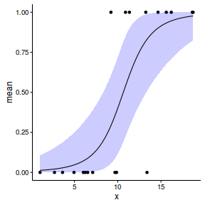
Grouped binomial regression (proportional counts)
Recall that the binomial distribution represents the density (probability) of all possible successes out of a total of N trials. Hence the binomial distribution is also a suitable error distribution for analysing grouped binary data. An example of group data might be the number of seeds that germinate out of a total of 10 seeds, or the number of female kangaroos with joeys out of a total of 120 female kangaroos.
For this demonstration, we will model the number of successes against a uniformly distributed predictor (x). The number of trials in each group (level of the predictor) will vary slightly (yet randomly) so as to mimic complications that inevitable occur in real experiments.
- the number of levels of $x$ = 10
- the continuous $x$ variable is a random uniform spread of measurements between 10 and 20
- the rate of change in log odds ratio per unit change in x (slope) = -0.25. The magnitude of the slope is an indicator of how abruptly the log odds ratio changes. A very abrupt change would occur if there was very little variability in the trend. That is, a large slope would be indicative of a threshold effect. A lower slope indicates a gradual change in odds ratio and thus a less obvious and precise switch between the likelihood of 1 vs 0.
- the inflection point (point where the slope of the line is greatest) = 10. The inflection point indicates the value of the predictor ($x$) where the log Odds are 50% (switching between 1 being more likely and 0 being more likely). This is also known as the LD50.
- the intercept (which has no real interpretation) is equal to the negative of the slope multiplied by the inflection point
- generate the values of $y$ expected at each $x$ value, we evaluate the linear predictor.
- generate random numbers of trials per group by drawing integers out of a binomial distribution with a total size of 20 and probability of 0.9. Hence the maximum number of trials per group will be 20, yet some will be less than that.
- the number of success per group are drawn from a binomial distribution with a total size equal to the trial sizes generated in the previous step and probabilities equal to the expected $y$ values
- finally, the number of failures per group are calculated as the difference between the total trial size and number of successes per group.
set.seed(8)
#The number of levels of x
n.x <- 10
#Create x values that at uniformly distributed throughout the rate of 10 to 20
x <- sort(runif(n = n.x, min = 10, max =20))
#The slope is the rate of change in log odds ratio for each unit change in x
# the smaller the slope, the slower the change (more variability in data too)
slope=-.25
#Inflection point is where the slope of the line is greatest
#this is also the LD50 point
inflect <- 15
#Intercept (no interpretation)
intercept <- -1*(slope*inflect)
#The linear predictor
linpred <- intercept+slope*x
#Predicted y values
y.pred <- exp(linpred)/(1+exp(linpred))
#Add some noise and make binary (0's and 1's)
n.trial <- rbinom(n=n.x,20, prob=0.9)
success <- rbinom(n = n.x, size = n.trial,prob = y.pred)
failure <- n.trial - success
dat <- data.frame(success,failure,x)
$$ log\left(\frac{\pi}{1-\pi}\right)=\beta_0+\beta_1x_1+\epsilon_i, \hspace{1cm}\epsilon\sim Binom(\lambda) $$
dat<-within(dat, total<-success+failure)
dat.glm <- glm(cbind(success,failure)~x, data=dat, family="binomial", weight=total)
summary(dat.glm)
Call:
glm(formula = cbind(success, failure) ~ x, family = "binomial",
    data = dat, weights = total)

Deviance Residuals:
    Min       1Q   Median       3Q      Max
-6.3073  -1.2530   0.5005   2.1157   5.8746

Coefficients:
            Estimate Std. Error z value Pr(>|z|)
(Intercept)   4.0472     0.2525   16.03   <2e-16 ***
x            -0.2591     0.0158  -16.40   <2e-16 ***
---
Signif. codes:  0 '***' 0.001 '**' 0.01 '*' 0.05 '.' 0.1 ' ' 1

(Dispersion parameter for binomial family taken to be 1)

    Null deviance: 394.60  on 9  degrees of freedom
Residual deviance: 105.33  on 8  degrees of freedom
AIC: 716.15

Number of Fisher Scoring iterations: 3
dat.list <- with(dat, list(success=success, total=success+failure, x=x, N=nrow(dat)))
modelString="
model{
  for (i in 1:N) {
    success[i] ~ dbin(p[i],total[i])
    logit(p[i]) <- max(-20,min(20,beta0+beta1*x[i]))
  }
  beta0 ~ dnorm(0,1.0E-06)
  beta1 ~ dnorm(0,1.0E-06)
}
"
writeLines(modelString, con='../downloads/BUGSscripts/tut11.4bS2.bug')
library(R2jags)
dat.logit.jags <- jags(data=dat.list,model.file='../downloads/BUGSscripts/tut11.4bS2.bug',
                   param=c('beta0','beta1'),
                   n.chains=3, n.iter=200000, n.burnin=100000, n.thin=100)
Compiling model graph
   Resolving undeclared variables
   Allocating nodes
   Graph Size: 87

Initializing model
print(dat.logit.jags)
Inference for Bugs model at "../downloads/BUGSscripts/tut11.4bS2.bug", fit using jags,
 3 chains, each with 2e+05 iterations (first 1e+05 discarded), n.thin = 100
 n.sims = 3000 iterations saved
         mu.vect sd.vect   2.5%    25%    50%    75%  97.5%  Rhat n.eff
beta0      4.008   1.086  1.892  3.305  3.972  4.753  6.148 1.002  1300
beta1     -0.256   0.068 -0.387 -0.302 -0.255 -0.210 -0.125 1.002  1300
deviance  40.637   1.984 38.680 39.218 40.011 41.478 45.896 1.001  3000

For each parameter, n.eff is a crude measure of effective sample size,
and Rhat is the potential scale reduction factor (at convergence, Rhat=1).

DIC info (using the rule, pD = var(deviance)/2)
pD = 2.0 and DIC = 42.6
DIC is an estimate of expected predictive error (lower deviance is better).
library(rstan)
modelString="
data {
   int<lower=1> n;
   int<lower=1> nX;
   int y[n];
   int nTrials[n];
   matrix [n,nX] X;
}
parameters {
   vector [nX] beta;
}
transformed parameters {
   vector [n] mu;
   mu<-X*beta;
}
model {
   beta ~ normal(0,1000);
   y ~ binomial_logit(nTrials, mu);
}
"
Xmat <- model.matrix(~x,data=dat)
dat.list <- with(dat, list(y = success, nTrials=success+failure, X = Xmat, nX=ncol(Xmat),n = nrow(dat)))

library(rstan)
dat.rstan <- stan(data=dat.list,
           model_code=modelString,
           chains=3,
           iter=1000,
           warmup=500,
                   thin=2,
           save_dso=TRUE
           )
SAMPLING FOR MODEL '6c0358c6c330110e714238536a9a5894' NOW (CHAIN 1).

Chain 1, Iteration:   1 / 1000 [  0%]  (Warmup)
Chain 1, Iteration: 100 / 1000 [ 10%]  (Warmup)
Chain 1, Iteration: 200 / 1000 [ 20%]  (Warmup)
Chain 1, Iteration: 300 / 1000 [ 30%]  (Warmup)
Chain 1, Iteration: 400 / 1000 [ 40%]  (Warmup)
Chain 1, Iteration: 500 / 1000 [ 50%]  (Warmup)
Chain 1, Iteration: 501 / 1000 [ 50%]  (Sampling)
Chain 1, Iteration: 600 / 1000 [ 60%]  (Sampling)
Chain 1, Iteration: 700 / 1000 [ 70%]  (Sampling)
Chain 1, Iteration: 800 / 1000 [ 80%]  (Sampling)
Chain 1, Iteration: 900 / 1000 [ 90%]  (Sampling)
Chain 1, Iteration: 1000 / 1000 [100%]  (Sampling)#
#  Elapsed Time: 0.060866 seconds (Warm-up)
#                0.032433 seconds (Sampling)
#                0.093299 seconds (Total)
#

SAMPLING FOR MODEL '6c0358c6c330110e714238536a9a5894' NOW (CHAIN 2).

Chain 2, Iteration:   1 / 1000 [  0%]  (Warmup)
Chain 2, Iteration: 100 / 1000 [ 10%]  (Warmup)
Chain 2, Iteration: 200 / 1000 [ 20%]  (Warmup)
Chain 2, Iteration: 300 / 1000 [ 30%]  (Warmup)
Chain 2, Iteration: 400 / 1000 [ 40%]  (Warmup)
Chain 2, Iteration: 500 / 1000 [ 50%]  (Warmup)
Chain 2, Iteration: 501 / 1000 [ 50%]  (Sampling)
Chain 2, Iteration: 600 / 1000 [ 60%]  (Sampling)
Chain 2, Iteration: 700 / 1000 [ 70%]  (Sampling)
Chain 2, Iteration: 800 / 1000 [ 80%]  (Sampling)
Chain 2, Iteration: 900 / 1000 [ 90%]  (Sampling)
Chain 2, Iteration: 1000 / 1000 [100%]  (Sampling)#
#  Elapsed Time: 0.055367 seconds (Warm-up)
#                0.038589 seconds (Sampling)
#                0.093956 seconds (Total)
#

SAMPLING FOR MODEL '6c0358c6c330110e714238536a9a5894' NOW (CHAIN 3).

Chain 3, Iteration:   1 / 1000 [  0%]  (Warmup)
Chain 3, Iteration: 100 / 1000 [ 10%]  (Warmup)
Chain 3, Iteration: 200 / 1000 [ 20%]  (Warmup)
Chain 3, Iteration: 300 / 1000 [ 30%]  (Warmup)
Chain 3, Iteration: 400 / 1000 [ 40%]  (Warmup)
Chain 3, Iteration: 500 / 1000 [ 50%]  (Warmup)
Chain 3, Iteration: 501 / 1000 [ 50%]  (Sampling)
Chain 3, Iteration: 600 / 1000 [ 60%]  (Sampling)
Chain 3, Iteration: 700 / 1000 [ 70%]  (Sampling)
Chain 3, Iteration: 800 / 1000 [ 80%]  (Sampling)
Chain 3, Iteration: 900 / 1000 [ 90%]  (Sampling)
Chain 3, Iteration: 1000 / 1000 [100%]  (Sampling)#
#  Elapsed Time: 0.126566 seconds (Warm-up)
#                0.072445 seconds (Sampling)
#                0.199011 seconds (Total)
#
print(dat.rstan, pars=c('beta'))
Inference for Stan model: 6c0358c6c330110e714238536a9a5894.
3 chains, each with iter=1000; warmup=500; thin=2;
post-warmup draws per chain=250, total post-warmup draws=750.

         mean se_mean   sd  2.5%   25%   50%   75% 97.5% n_eff Rhat
beta[1]  4.16    0.07 1.08  2.07  3.41  4.19  4.84  6.34   219 1.00
beta[2] -0.26    0.00 0.07 -0.39 -0.31 -0.27 -0.22 -0.13   217 1.01

Samples were drawn using NUTS(diag_e) at Mon Feb 22 12:12:59 2016.
For each parameter, n_eff is a crude measure of effective sample size,
and Rhat is the potential scale reduction factor on split chains (at
convergence, Rhat=1).
library(brms)
dat<-within(dat, total<-success+failure)
dat.brm <- brm(success|trials(total)~x, data=dat, family='binomial',
   prior=c(set_prior('normal(0,1000)', class='b')),
   n.chains=3, n.iter=1000, warmup=500, n.thin=2
)
SAMPLING FOR MODEL 'binomial(logit) brms-model' NOW (CHAIN 1).

Chain 1, Iteration:   1 / 1000 [  0%]  (Warmup)
Chain 1, Iteration: 100 / 1000 [ 10%]  (Warmup)
Chain 1, Iteration: 200 / 1000 [ 20%]  (Warmup)
Chain 1, Iteration: 300 / 1000 [ 30%]  (Warmup)
Chain 1, Iteration: 400 / 1000 [ 40%]  (Warmup)
Chain 1, Iteration: 500 / 1000 [ 50%]  (Warmup)
Chain 1, Iteration: 501 / 1000 [ 50%]  (Sampling)
Chain 1, Iteration: 600 / 1000 [ 60%]  (Sampling)
Chain 1, Iteration: 700 / 1000 [ 70%]  (Sampling)
Chain 1, Iteration: 800 / 1000 [ 80%]  (Sampling)
Chain 1, Iteration: 900 / 1000 [ 90%]  (Sampling)
Chain 1, Iteration: 1000 / 1000 [100%]  (Sampling)#
#  Elapsed Time: 0.061524 seconds (Warm-up)
#                0.040658 seconds (Sampling)
#                0.102182 seconds (Total)
#

SAMPLING FOR MODEL 'binomial(logit) brms-model' NOW (CHAIN 2).

Chain 2, Iteration:   1 / 1000 [  0%]  (Warmup)
Chain 2, Iteration: 100 / 1000 [ 10%]  (Warmup)
Chain 2, Iteration: 200 / 1000 [ 20%]  (Warmup)
Chain 2, Iteration: 300 / 1000 [ 30%]  (Warmup)
Chain 2, Iteration: 400 / 1000 [ 40%]  (Warmup)
Chain 2, Iteration: 500 / 1000 [ 50%]  (Warmup)
Chain 2, Iteration: 501 / 1000 [ 50%]  (Sampling)
Chain 2, Iteration: 600 / 1000 [ 60%]  (Sampling)
Chain 2, Iteration: 700 / 1000 [ 70%]  (Sampling)
Chain 2, Iteration: 800 / 1000 [ 80%]  (Sampling)
Chain 2, Iteration: 900 / 1000 [ 90%]  (Sampling)
Chain 2, Iteration: 1000 / 1000 [100%]  (Sampling)#
#  Elapsed Time: 0.073432 seconds (Warm-up)
#                0.039209 seconds (Sampling)
#                0.112641 seconds (Total)
#

SAMPLING FOR MODEL 'binomial(logit) brms-model' NOW (CHAIN 3).

Chain 3, Iteration:   1 / 1000 [  0%]  (Warmup)
Chain 3, Iteration: 100 / 1000 [ 10%]  (Warmup)
Chain 3, Iteration: 200 / 1000 [ 20%]  (Warmup)
Chain 3, Iteration: 300 / 1000 [ 30%]  (Warmup)
Chain 3, Iteration: 400 / 1000 [ 40%]  (Warmup)
Chain 3, Iteration: 500 / 1000 [ 50%]  (Warmup)
Chain 3, Iteration: 501 / 1000 [ 50%]  (Sampling)
Chain 3, Iteration: 600 / 1000 [ 60%]  (Sampling)
Chain 3, Iteration: 700 / 1000 [ 70%]  (Sampling)
Chain 3, Iteration: 800 / 1000 [ 80%]  (Sampling)
Chain 3, Iteration: 900 / 1000 [ 90%]  (Sampling)
Chain 3, Iteration: 1000 / 1000 [100%]  (Sampling)#
#  Elapsed Time: 0.061522 seconds (Warm-up)
#                0.036074 seconds (Sampling)
#                0.097596 seconds (Total)
#
summary(dat.brm)
 Family: binomial (logit)
Formula: success | trials(total) ~ x
   Data: dat (Number of observations: 10)
Samples: 3 chains, each with n.iter = 1000; n.warmup = 500; n.thin = 2;
         total post-warmup samples = 750
   WAIC: 41.57

Fixed Effects:
          Estimate Est.Error l-95% CI u-95% CI Eff.Sample Rhat
Intercept     4.10      1.00     2.24     6.00        200    1
x            -0.26      0.06    -0.38    -0.14        200    1

Samples were drawn using NUTS(diag_e). For each parameter, Eff.Sample is a
crude measure of effective sample size, and Rhat is the potential scale
reduction factor on split chains (at convergence, Rhat = 1).
stancode(dat.brm)
functions {
}
data {
  int<lower=1> N;  # number of observations
  int Y[N];  # response variable
  int<lower=1> K;  # number of fixed effects
  matrix[N, K] X;  # FE design matrix
  int trials[N];  # number of trials
}
transformed data {
}
parameters {
  real b_Intercept;  # fixed effects Intercept
  vector[K] b;  # fixed effects
}
transformed parameters {
  vector[N] eta;  # linear predictor
  # compute linear predictor
  eta <- X * b + b_Intercept;
}
model {
  # prior specifications
  b_Intercept ~ normal(0,1000);
  b ~ normal(0,1000);
  # likelihood contribution
  Y ~ binomial_logit(trials, eta);
}
generated quantities {
}
fitted <- subset(dat, select=c(x,success,failure,total))
fitted$success <- NA
newdata <- expand.grid(success=NA, failure=NA,x=seq(min(dat$x), max(dat$x), len=100), total=NA)
dat.pred <- rbind(dat,fitted,newdata)
Now lets fit the model.
#fit the model
dat.inla <- inla(success~x, family='binomial',Ntrials=total,
   data=dat.pred,
   control.family=list(link='logit'),
   control.predictor=list(link=1, compute=TRUE),
   control.compute=list(dic=TRUE, cpo=TRUE, waic=TRUE))
#examine the regular summary
summary(dat.inla)
Call:
c("inla(formula = success ~ x, family = \"binomial\", data = dat.pred, ",  "    Ntrials = total, control.compute = list(dic = TRUE, cpo = TRUE, ",  "        waic = TRUE), control.predictor = list(link = 1, compute = TRUE), ",  "    control.family = list(link = \"logit\"))")

Time used:
 Pre-processing    Running inla Post-processing           Total
         0.0825          0.0438          0.0288          0.1551

Fixed effects:
               mean    sd 0.025quant 0.5quant 0.975quant    mode kld
(Intercept)  4.0391 1.088     1.9497   4.0230     6.2217  3.9907   0
x           -0.2577 0.068    -0.3940  -0.2567    -0.1266 -0.2548   0

The model has no random effects

The model has no hyperparameters

Expected number of effective parameters(std dev): 2.001(0.00)
Number of equivalent replicates : 4.999

Deviance Information Criterion (DIC) ...: 42.59
Effective number of parameters .........: 1.987

Watanabe-Akaike information criterion (WAIC) ...: 41.93
Effective number of parameters .................: 1.15

Marginal log-Likelihood:  -26.41
CPO and PIT are computed

Posterior marginals for linear predictor and fitted values computed
newdata <- cbind(newdata,
  dat.inla$summary.fitted.values[(nrow(dat)+nrow(fitted)+1):nrow(dat.pred),])
head(newdata)
                     success failure        x total      mean         sd 0.025quant  0.5quant 0.975quant
fitted.predictor.021      NA      NA 12.07823    NA 0.7125421 0.05985063  0.5878929 0.7153579  0.8212576
fitted.predictor.022      NA      NA 12.15141    NA 0.7088373 0.05946393  0.5852983 0.7115181  0.8171994
fitted.predictor.023      NA      NA 12.22459    NA 0.7050996 0.05906512  0.5826879 0.7076480  0.8130769
fitted.predictor.024      NA      NA 12.29776    NA 0.7013292 0.05865439  0.5800613 0.7037477  0.8088906
fitted.predictor.025      NA      NA 12.37094    NA 0.6975263 0.05823199  0.5774180 0.6998179  0.8046408
fitted.predictor.026      NA      NA 12.44412    NA 0.6936912 0.05779817  0.5747575 0.6958587  0.8003281
                          mode
fitted.predictor.021 0.7212332
fitted.predictor.022 0.7171021
fitted.predictor.023 0.7129469
fitted.predictor.024 0.7087681
fitted.predictor.025 0.7045663
fitted.predictor.026 0.7003420
newdata <- reshape:::rename(newdata, c("0.025quant"="lower", "0.975quant"="upper"))

#fitted <- cbind(fitted,
#  dat.inla$summary.fitted.values[(nrow(dat)+1):(nrow(dat)+nrow(fitted)),])
#fitted <- reshape:::rename(fitted, c("0.025quant"="lower", "0.975quant"="upper"))

#fitted$partial.obs=fitted$mean + (fitted$mean - dat$y)

library(grid)
ggplot(newdata, aes(y=mean, x=x)) +
        geom_blank()+
        geom_point(data=dat, aes(y=I(success/total), x=x)) +
        geom_ribbon(aes(ymin=lower, ymax=upper), fill='blue', alpha=0.2) +
        geom_line() +
        scale_y_continuous('Probability of success')+
        theme_classic()+
        theme(legend.key.width=unit(2,'lines'), legend.position=c(0,1), legend.justification=c(0,1),
              axis.title.y=element_text(margin(r=2,unit='lines')))
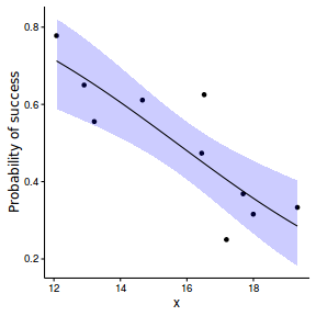
Beta regression (percent cover)
Percent cover (or any percentage for that matter) can logically only range from 0 to 1 (0, 100%). When the observed values are sufficiently away from either 0 and 1, a Gaussian distribution might be effective. However, when observations are close to 0 or 1, Gaussian based models are likely to be poor representations of the true situation at these boundaries. Indeed, predictions close to these boundaries (or the confidence intervals) may actually fall outside the logical range.
The beta distribution is defined for any real number between 0 and 1. The beta distribution is a relatively complex modelling distribution as it can take on a variety of forms. As with models that incorporate a binomial distribution, the beta distribution is typically associated with a logit link function.
- the number of levels of $x$ = 10
- the continuous $x$ variable is a random uniform spread of measurements between 10 and 20
- the rate of change in log odds ratio per unit change in x (slope) = -0.8. The magnitude of the slope is an indicator of how abruptly the log odds ratio changes. A very abrupt change would occur if there was very little variability in the trend. That is, a large slope would be indicative of a threshold effect. A lower slope indicates a gradual change in odds ratio and thus a less obvious and precise switch between the likelihood of 1 vs 0.
- the inflection point (point where the slope of the line is greatest) = 16. The inflection point indicates the value of the predictor ($x$) where the log Odds are 50% (switching between 1 being more likely and 0 being more likely). This is also known as the LD50.
- the intercept (which has no real interpretation) is equal to the negative of the slope multiplied by the inflection point
- generate the values of $y$ expected at each $x$ value, we evaluate the linear predictor.
- generate percentage cover observations by drawing values from a beta distribution with shape parameters defined according to: $$ \begin{align} \text{shape1} (\alpha) &=\Bigg(\frac{1-\mu}{\sigma^2} - \frac{1}{\mu}\Bigg)\\ \text{shape2} (\beta) &=\alpha\Bigg(\frac{1}{\mu} - 1 \Bigg)\\ \end{align} $$ these cover values are expressed as proportions rather than percentages since values need to be between 0 and 1. The mean ($\mu$) is determined by the linear predictor and the variance ($\sigma^2) we will nominate as 0.01.
set.seed(8)
#The number of levels of x
n.x <- 10
#Create x values that at uniformly distributed throughout the rate of 10 to 20
x <- sort(runif(n = n.x, min = 10, max =20))
slope=-.8
#Inflection point is where the slope of the line is greatest
#this is also the LD50 point
inflect <- 16
#Intercept (no interpretation)
intercept <- -1*(slope*inflect)
#The linear predictor
linpred <- intercept+slope*x
y.pred <- exp(linpred)/(1+exp(linpred))
sigma=0.01
estBetaParams <- function(mu, var) {
  alpha <- ((1 - mu) / var - 1 / mu) * mu ^ 2
  beta <- alpha * (1 / mu - 1)
  return(params = list(alpha = alpha, beta = beta))
}
betaShapes=estBetaParams(y.pred, sigma)
y=rbeta(n=n.x, shape1=betaShapes$alpha, shape2=betaShapes$beta)
dat <- data.frame(y,x)
$$ \begin{align} log\left(\frac{\pi}{1-\pi}\right)&=\beta_0+\beta_1x_1+\epsilon_i, \hspace{1cm}\epsilon\sim Beta(\alpha, \beta)\\ \alpha &=\Bigg(\frac{1-\mu}{\sigma^2} - \frac{1}{\mu}\Bigg)\\ \beta &=\alpha\Bigg(\frac{1}{\mu} - 1 \Bigg)\\ \end{align} $$
library(betareg)
dat.glm <- betareg(y~x, data=dat)
summary(dat.glm)
Call:
betareg(formula = y ~ x, data = dat)

Standardized weighted residuals 2:
    Min      1Q  Median      3Q     Max
-2.9455 -0.9286 -0.0994  0.9147  1.3906

Coefficients (mean model with logit link):
            Estimate Std. Error z value Pr(>|z|)
(Intercept)  11.7680     2.0298   5.798 6.72e-09 ***
x            -0.7634     0.1281  -5.957 2.57e-09 ***

Phi coefficients (precision model with identity link):
      Estimate Std. Error z value Pr(>|z|)
(phi)    9.427      4.278   2.204   0.0275 *
---
Signif. codes:  0 '***' 0.001 '**' 0.01 '*' 0.05 '.' 0.1 ' ' 1

Type of estimator: ML (maximum likelihood)
Log-likelihood: 12.96 on 3 Df
Pseudo R-squared: 0.6214
Number of iterations: 32 (BFGS) + 8 (Fisher scoring)
modelString="
model{
  for (i in 1:N) {
    y[i] ~ dbeta(a[i],b[i])
    a[i] <- eta[i] * phi
    b[i] <- (1 - eta[i]) * phi
    logit(eta[i]) <- beta0+beta1*x[i]
  }
  beta0 ~ dnorm(0,1.0E-06)
  beta1 ~ dnorm(0,1.0E-06)
  phi ~ dgamma(0.01, 0.01)
}
"
library(R2jags)
dat.list <- with(dat, list(y=y, x=x, N=nrow(dat)))
dat.jags <- jags(data=dat.list,model.file=textConnection(modelString),
                   param=c('beta0','beta1','phi'),
                   n.chains=3, n.iter=20000, n.burnin=10000, n.thin=100)
Compiling model graph
   Resolving undeclared variables
   Allocating nodes
   Graph Size: 88

Initializing model
print(dat.jags)
Inference for Bugs model at "5", fit using jags,
 3 chains, each with 20000 iterations (first 10000 discarded), n.thin = 100
 n.sims = 300 iterations saved
         mu.vect sd.vect    2.5%     25%     50%     75%   97.5%  Rhat n.eff
beta0     11.783   2.378   7.636  10.183  11.458  13.363  16.476 1.020   120
beta1     -0.764   0.143  -1.052  -0.856  -0.753  -0.668  -0.500 1.026    90
phi        8.832   4.228   2.579   5.747   8.345  11.059  19.175 1.002   300
deviance -22.691   2.689 -25.702 -24.548 -23.459 -21.564 -15.303 1.025   250

For each parameter, n.eff is a crude measure of effective sample size,
and Rhat is the potential scale reduction factor (at convergence, Rhat=1).

DIC info (using the rule, pD = var(deviance)/2)
pD = 3.6 and DIC = -19.1
DIC is an estimate of expected predictive error (lower deviance is better).
library(rstan)
modelString="
data {
  int<lower=1> n;  // number of observations
  vector[n] y;  // response variable
  int<lower=1> nX;  // number of fixed effects
  matrix[n, nX] X;  // FE design matrix
}
transformed data {
}
parameters {
  vector[nX] beta;  // fixed effects
  real<lower=0> phi;  // precision parameter
}
transformed parameters {
  vector[n] eta;  // linear predictor
  // compute linear predictor
  eta <- X * beta;
  for (i in 1:n) {
    eta[i] <- inv_logit(eta[i]);
  }
}
model {
  // prior specifications
  phi ~ gamma(0.01, 0.01);
  beta ~ normal(0, 1000);
  // likelihood contribution
  y ~ beta(eta * phi, (1 - eta) * phi);
}
generated quantities {
}
"
Xmat <- model.matrix(~x,data=dat)
dat.list <- with(dat, list(y = y, X = Xmat,nX=ncol(Xmat),n = nrow(dat)))


library(rstan)
dat.rstan <- stan(data=dat.list,
           model_code=modelString,
           chains=3,
           iter=1000,
           warmup=500,
                   thin=2,
           save_dso=TRUE
           )
SAMPLING FOR MODEL 'd261ea666f0b7a9209e5feedf9d26f12' NOW (CHAIN 1).

Chain 1, Iteration:   1 / 1000 [  0%]  (Warmup)
Chain 1, Iteration: 100 / 1000 [ 10%]  (Warmup)
Chain 1, Iteration: 200 / 1000 [ 20%]  (Warmup)
Chain 1, Iteration: 300 / 1000 [ 30%]  (Warmup)
Chain 1, Iteration: 400 / 1000 [ 40%]  (Warmup)
Chain 1, Iteration: 500 / 1000 [ 50%]  (Warmup)
Chain 1, Iteration: 501 / 1000 [ 50%]  (Sampling)
Chain 1, Iteration: 600 / 1000 [ 60%]  (Sampling)
Chain 1, Iteration: 700 / 1000 [ 70%]  (Sampling)
Chain 1, Iteration: 800 / 1000 [ 80%]  (Sampling)
Chain 1, Iteration: 900 / 1000 [ 90%]  (Sampling)
Chain 1, Iteration: 1000 / 1000 [100%]  (Sampling)#
#  Elapsed Time: 0.250474 seconds (Warm-up)
#                0.133006 seconds (Sampling)
#                0.38348 seconds (Total)
#

SAMPLING FOR MODEL 'd261ea666f0b7a9209e5feedf9d26f12' NOW (CHAIN 2).

Chain 2, Iteration:   1 / 1000 [  0%]  (Warmup)
Chain 2, Iteration: 100 / 1000 [ 10%]  (Warmup)
Chain 2, Iteration: 200 / 1000 [ 20%]  (Warmup)
Chain 2, Iteration: 300 / 1000 [ 30%]  (Warmup)
Chain 2, Iteration: 400 / 1000 [ 40%]  (Warmup)
Chain 2, Iteration: 500 / 1000 [ 50%]  (Warmup)
Chain 2, Iteration: 501 / 1000 [ 50%]  (Sampling)
Chain 2, Iteration: 600 / 1000 [ 60%]  (Sampling)
Chain 2, Iteration: 700 / 1000 [ 70%]  (Sampling)
Chain 2, Iteration: 800 / 1000 [ 80%]  (Sampling)
Chain 2, Iteration: 900 / 1000 [ 90%]  (Sampling)
Chain 2, Iteration: 1000 / 1000 [100%]  (Sampling)#
#  Elapsed Time: 0.255301 seconds (Warm-up)
#                0.200749 seconds (Sampling)
#                0.45605 seconds (Total)
#

SAMPLING FOR MODEL 'd261ea666f0b7a9209e5feedf9d26f12' NOW (CHAIN 3).

Chain 3, Iteration:   1 / 1000 [  0%]  (Warmup)
Chain 3, Iteration: 100 / 1000 [ 10%]  (Warmup)
Chain 3, Iteration: 200 / 1000 [ 20%]  (Warmup)
Chain 3, Iteration: 300 / 1000 [ 30%]  (Warmup)
Chain 3, Iteration: 400 / 1000 [ 40%]  (Warmup)
Chain 3, Iteration: 500 / 1000 [ 50%]  (Warmup)
Chain 3, Iteration: 501 / 1000 [ 50%]  (Sampling)
Chain 3, Iteration: 600 / 1000 [ 60%]  (Sampling)
Chain 3, Iteration: 700 / 1000 [ 70%]  (Sampling)
Chain 3, Iteration: 800 / 1000 [ 80%]  (Sampling)
Chain 3, Iteration: 900 / 1000 [ 90%]  (Sampling)
Chain 3, Iteration: 1000 / 1000 [100%]  (Sampling)#
#  Elapsed Time: 0.292455 seconds (Warm-up)
#                0.172565 seconds (Sampling)
#                0.46502 seconds (Total)
#
print(dat.rstan, pars=c('beta','phi'))
Inference for Stan model: d261ea666f0b7a9209e5feedf9d26f12.
3 chains, each with iter=1000; warmup=500; thin=2;
post-warmup draws per chain=250, total post-warmup draws=750.

         mean se_mean   sd  2.5%   25%   50%   75% 97.5% n_eff Rhat
beta[1] 11.72    0.15 2.47  6.40 10.14 11.69 13.35 16.37   289 1.01
beta[2] -0.76    0.01 0.15 -1.05 -0.86 -0.76 -0.67 -0.43   283 1.01
phi      7.86    0.17 3.02  2.55  5.72  7.62  9.81 14.15   321 1.00

Samples were drawn using NUTS(diag_e) at Mon Feb 22 21:30:57 2016.
For each parameter, n_eff is a crude measure of effective sample size,
and Rhat is the potential scale reduction factor on split chains (at
convergence, Rhat=1).
library(brms)
dat.brm <- brm(y~x, data=dat, family='beta',
   prior=c(set_prior('normal(0,1000)', class='b')),
   n.chains=3, n.iter=1000, warmup=500, n.thin=2
)
SAMPLING FOR MODEL 'beta(logit) brms-model' NOW (CHAIN 1).

Chain 1, Iteration:   1 / 1000 [  0%]  (Warmup)
Chain 1, Iteration: 100 / 1000 [ 10%]  (Warmup)
Chain 1, Iteration: 200 / 1000 [ 20%]  (Warmup)
Chain 1, Iteration: 300 / 1000 [ 30%]  (Warmup)
Chain 1, Iteration: 400 / 1000 [ 40%]  (Warmup)
Chain 1, Iteration: 500 / 1000 [ 50%]  (Warmup)
Chain 1, Iteration: 501 / 1000 [ 50%]  (Sampling)
Chain 1, Iteration: 600 / 1000 [ 60%]  (Sampling)
Chain 1, Iteration: 700 / 1000 [ 70%]  (Sampling)
Chain 1, Iteration: 800 / 1000 [ 80%]  (Sampling)
Chain 1, Iteration: 900 / 1000 [ 90%]  (Sampling)
Chain 1, Iteration: 1000 / 1000 [100%]  (Sampling)#
#  Elapsed Time: 7.54483 seconds (Warm-up)
#                17.3168 seconds (Sampling)
#                24.8616 seconds (Total)
#

SAMPLING FOR MODEL 'beta(logit) brms-model' NOW (CHAIN 2).

Chain 2, Iteration:   1 / 1000 [  0%]  (Warmup)
Chain 2, Iteration: 100 / 1000 [ 10%]  (Warmup)
Chain 2, Iteration: 200 / 1000 [ 20%]  (Warmup)
Chain 2, Iteration: 300 / 1000 [ 30%]  (Warmup)
Chain 2, Iteration: 400 / 1000 [ 40%]  (Warmup)
Chain 2, Iteration: 500 / 1000 [ 50%]  (Warmup)
Chain 2, Iteration: 501 / 1000 [ 50%]  (Sampling)
Chain 2, Iteration: 600 / 1000 [ 60%]  (Sampling)
Chain 2, Iteration: 700 / 1000 [ 70%]  (Sampling)
Chain 2, Iteration: 800 / 1000 [ 80%]  (Sampling)
Chain 2, Iteration: 900 / 1000 [ 90%]  (Sampling)
Chain 2, Iteration: 1000 / 1000 [100%]  (Sampling)#
#  Elapsed Time: 0.112244 seconds (Warm-up)
#                0.056446 seconds (Sampling)
#                0.16869 seconds (Total)
#

SAMPLING FOR MODEL 'beta(logit) brms-model' NOW (CHAIN 3).

Chain 3, Iteration:   1 / 1000 [  0%]  (Warmup)
Chain 3, Iteration: 100 / 1000 [ 10%]  (Warmup)
Chain 3, Iteration: 200 / 1000 [ 20%]  (Warmup)
Chain 3, Iteration: 300 / 1000 [ 30%]  (Warmup)
Chain 3, Iteration: 400 / 1000 [ 40%]  (Warmup)
Chain 3, Iteration: 500 / 1000 [ 50%]  (Warmup)
Chain 3, Iteration: 501 / 1000 [ 50%]  (Sampling)
Chain 3, Iteration: 600 / 1000 [ 60%]  (Sampling)
Chain 3, Iteration: 700 / 1000 [ 70%]  (Sampling)
Chain 3, Iteration: 800 / 1000 [ 80%]  (Sampling)
Chain 3, Iteration: 900 / 1000 [ 90%]  (Sampling)
Chain 3, Iteration: 1000 / 1000 [100%]  (Sampling)#
#  Elapsed Time: 0.085228 seconds (Warm-up)
#                0.061105 seconds (Sampling)
#                0.146333 seconds (Total)
#
summary(dat.brm)
 Family: beta (logit)
Formula: y ~ x
   Data: dat (Number of observations: 10)
Samples: 3 chains, each with iter = 1000; warmup = 500; thin = 2;
         total post-warmup samples = 750
   WAIC: Not computed

Fixed Effects:
          Estimate Est.Error l-95% CI u-95% CI Eff.Sample Rhat
Intercept    13.43      3.26     7.56    18.08          2 1.77
x            -0.86      0.19    -1.13    -0.50          2 1.70

Family Specific Parameters:
    Estimate Est.Error l-95% CI u-95% CI Eff.Sample Rhat
phi    19.82     17.26     3.08    49.04          2 5.94

Samples were drawn using sampling(NUTS). For each parameter, Eff.Sample
is a crude measure of effective sample size, and Rhat is the potential
scale reduction factor on split chains (at convergence, Rhat = 1).
stancode(dat.brm)
functions {
}
data {
  int<lower=1> N;  // number of observations
  vector[N] Y;  // response variable
  int<lower=1> K;  // number of fixed effects
  matrix[N, K] X;  // FE design matrix
  vector[K] X_means;  // column means of X
}
transformed data {
}
parameters {
  real temp_Intercept;  // temporary Intercept
  vector[K] b;  // fixed effects
  real<lower=0> phi;  // precision parameter
}
transformed parameters {
  vector[N] eta;  // linear predictor
  // compute linear predictor
  eta <- X * b + temp_Intercept;
  for (n in 1:N) {
    eta[n] <- inv_logit(eta[n]);
  }
}
model {
  // prior specifications
  b ~ normal(0,1000);
  phi ~ gamma(0.01, 0.01);
  // likelihood contribution
  Y ~ beta(eta * phi, (1 - eta) * phi);
}
generated quantities {
  real b_Intercept;  // fixed effects intercept
  b_Intercept <- temp_Intercept - dot_product(X_means, b);
}
fitted <- subset(dat, select=c(x,y))
fitted$y <- NA
newdata <- expand.grid(x=seq(min(dat$x), max(dat$x), len=100), y=NA)
dat.pred <- rbind(dat,fitted,newdata)
Now lets fit the model.
#fit the model
library(INLA)
dat.inla <- inla(y~x, family='beta',
   data=dat.pred,
   control.family=list(link='logit'),
   control.predictor=list(link=1, compute=TRUE),
   control.compute=list(dic=TRUE, cpo=TRUE, waic=TRUE))
#examine the regular summary
summary(dat.inla)
Call:
c("inla(formula = y ~ x, family = \"beta\", data = dat.pred, control.compute = list(dic = TRUE, ",  "    cpo = TRUE, waic = TRUE), control.predictor = list(link = 1, ",  "    compute = TRUE), control.family = list(link = \"logit\"))" )

Time used:
 Pre-processing    Running inla Post-processing           Total
         0.0695          0.0710          0.0248          0.1653

Fixed effects:
               mean     sd 0.025quant 0.5quant 0.975quant    mode kld
(Intercept) 11.6845 2.0768     7.7662  11.6131    15.9882 11.4692   0
x           -0.7599 0.1252    -1.0177  -0.7562    -0.5220 -0.7488   0

The model has no random effects

Model hyperparameters:
                                               mean    sd 0.025quant 0.5quant 0.975quant  mode
precision parameter for the beta observations 8.711 3.662      3.357    8.142      17.46 6.989

Expected number of effective parameters(std dev): 2.00(0.00)
Number of equivalent replicates : 5.00

Deviance Information Criterion (DIC) ...: -21.16
Effective number of parameters .........: 2.456

Watanabe-Akaike information criterion (WAIC) ...: -20.19
Effective number of parameters .................: 2.797

Marginal log-Likelihood:  5.913
CPO and PIT are computed

Posterior marginals for linear predictor and fitted values computed
newdata <- cbind(newdata,
  dat.inla$summary.fitted.values[(nrow(dat)+nrow(fitted)+1):nrow(dat.pred),])
head(newdata)
                            x  y      mean         sd 0.025quant  0.5quant 0.975quant      mode
fitted.predictor.021 12.07823 NA 0.9140861 0.04629234  0.7996400 0.9228020  0.9775402 0.9387765
fitted.predictor.022 12.15141 NA 0.9100518 0.04750029  0.7931865 0.9187774  0.9758870 0.9348454
fitted.predictor.023 12.22459 NA 0.9058414 0.04871891  0.7865733 0.9145631  0.9741167 0.9307015
fitted.predictor.024 12.29776 NA 0.9014486 0.04994645  0.7797996 0.9101522  0.9722216 0.9263219
fitted.predictor.025 12.37094 NA 0.8968674 0.05118101  0.7728648 0.9055379  0.9701937 0.9217106
fitted.predictor.026 12.44412 NA 0.8920916 0.05242054  0.7657683 0.9007135  0.9680244 0.9168501
newdata <- reshape:::rename(newdata, c("0.025quant"="lower", "0.975quant"="upper"))

library(grid)
ggplot(newdata, aes(y=mean*100, x=x)) +
        geom_blank()+
        geom_point(data=dat, aes(y=y*100, x=x)) +
        geom_ribbon(aes(ymin=lower*100, ymax=upper*100), fill='blue', alpha=0.2) +
        geom_line() +
        scale_y_continuous(expression(Cover~abundance~('%')))+
        theme_classic()+
        theme(legend.key.width=unit(2,'lines'), legend.position=c(0,1), legend.justification=c(0,1))
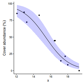
Poisson regression (count data)
Lets say we wanted to model the abundance of an item ($y$) against a continuous predictor ($x$). As this section is mainly about the generation of artificial data (and not specifically about what to do with the data), understanding the actual details are optional and can be safely skipped. Consequently, I have folded (toggled) this section away.
- the sample size = 20
- the continuous $x$ variable is a random uniform spread of measurements between 1 and 20
- the rate of change in log $y$ per unit of $x$ (slope) = 0.1.
- the value of $x$ when log$y$ equals 0 (when $y$=1)
- to generate the values of $y$ expected at each $x$ value, we evaluate the linear predictor (created by calculating the outer product of the model matrix and the regression parameters). These expected values are then transformed into a scale mapped by (0,$\infty$) by using the log function $e^{linear~predictor}$
- finally, we generate $y$ values by using the expected $y$ values ($\lambda$) as probabilities when drawing random numbers from a Poisson distribution. This step adds random noise to the expected $y$ values and returns only 0's and positive integers.
set.seed(8)
#The number of samples
n.x <- 20
#Create x values that at uniformly distributed throughout the rate of 1 to 20
x <- sort(runif(n = n.x, min = 1, max =20))
mm <- model.matrix(~x)
intercept <- 0.6
slope=0.1
#The linear predictor
linpred <- mm %*% c(intercept,slope)
#Predicted y values
lambda <- exp(linpred)
#Add some noise and make binomial
y <- rpois(n=n.x, lambda=lambda)
dat <- data.frame(y,x)
data.pois <- dat
$$ \begin{align} y_i &\sim{} Pois(\lambda_i)\\ log(\lambda_i)&=\beta_0+\beta_1x_1\\ \end{align} $$
dat.glm <- glm(y~x, data=data.pois, family="poisson")
summary(dat.glm)
Call:
glm(formula = y ~ x, family = "poisson", data = data.pois)

Deviance Residuals:
    Min       1Q   Median       3Q      Max
-1.6353  -0.7049   0.0440   0.5624   2.0457

Coefficients:
            Estimate Std. Error z value Pr(>|z|)
(Intercept)  0.56002    0.25395   2.205   0.0274 *
x            0.11151    0.01858   6.000 1.97e-09 ***
---
Signif. codes:  0 '***' 0.001 '**' 0.01 '*' 0.05 '.' 0.1 ' ' 1

(Dispersion parameter for poisson family taken to be 1)

    Null deviance: 55.614  on 19  degrees of freedom
Residual deviance: 17.226  on 18  degrees of freedom
AIC: 90.319

Number of Fisher Scoring iterations: 4
modelString="
model{
  for (i in 1:N) {
    y[i] ~ dpois(lambda[i])
    log(lambda[i]) <- max(-20,min(20,beta0+beta1*x[i]))
  }
  beta0 ~ dnorm(0,1.0E-06)
  beta1 ~ dnorm(0,1.0E-06)
}
"
dat.list <- with(data.pois, list(y=y, x=x, N=nrow(data.pois)))
dat.jags <- jags(data=dat.list,model.file=textConnection(modelString),
                   param=c('beta0','beta1'),
                   n.chains=3, n.iter=20000, n.burnin=10000, n.thin=100)
Compiling model graph
   Resolving undeclared variables
   Allocating nodes
   Graph Size: 147

Initializing model
print(dat.jags)
Inference for Bugs model at "5", fit using jags,
 3 chains, each with 20000 iterations (first 10000 discarded), n.thin = 100
 n.sims = 300 iterations saved
         mu.vect sd.vect   2.5%    25%    50%    75%  97.5%  Rhat n.eff
beta0      0.556   0.246  0.077  0.407  0.533  0.718  1.088 1.009   300
beta1      0.111   0.018  0.073  0.099  0.111  0.124  0.143 1.007   300
deviance  88.241   1.734 86.376 86.873 87.781 89.023 92.674 1.000   300

For each parameter, n.eff is a crude measure of effective sample size,
and Rhat is the potential scale reduction factor (at convergence, Rhat=1).

DIC info (using the rule, pD = var(deviance)/2)
pD = 1.5 and DIC = 89.8
DIC is an estimate of expected predictive error (lower deviance is better).
library(rstan)
modelString="
data {
   int<lower=1> n;
   int<lower=1> nX;
   int y[n];
   matrix [n,nX] X;
}
parameters {
   vector [nX] beta;
}
transformed parameters {
   vector [n] mu;
   mu<-X*beta;
}
model {
   beta ~ normal(0,1000);
   y ~ poisson_log(mu);
}
"
Xmat <- model.matrix(~x,data=data.pois)
dat.list <- with(data.pois, list(y = y, X = Xmat, nX=ncol(Xmat),n = nrow(data.pois)))

library(rstan)
dat.rstan <- stan(data=dat.list,
           model_code=modelString,
           chains=3,
           iter=1000,
           warmup=500,
                   thin=2,
           save_dso=TRUE
           )
SAMPLING FOR MODEL '95c0e3e05517b98739c4f0c17ec17bdd' NOW (CHAIN 1).

Chain 1, Iteration:   1 / 1000 [  0%]  (Warmup)
Chain 1, Iteration: 100 / 1000 [ 10%]  (Warmup)
Chain 1, Iteration: 200 / 1000 [ 20%]  (Warmup)
Chain 1, Iteration: 300 / 1000 [ 30%]  (Warmup)
Chain 1, Iteration: 400 / 1000 [ 40%]  (Warmup)
Chain 1, Iteration: 500 / 1000 [ 50%]  (Warmup)
Chain 1, Iteration: 501 / 1000 [ 50%]  (Sampling)
Chain 1, Iteration: 600 / 1000 [ 60%]  (Sampling)
Chain 1, Iteration: 700 / 1000 [ 70%]  (Sampling)
Chain 1, Iteration: 800 / 1000 [ 80%]  (Sampling)
Chain 1, Iteration: 900 / 1000 [ 90%]  (Sampling)
Chain 1, Iteration: 1000 / 1000 [100%]  (Sampling)#
#  Elapsed Time: 0.086074 seconds (Warm-up)
#                0.040789 seconds (Sampling)
#                0.126863 seconds (Total)
#

SAMPLING FOR MODEL '95c0e3e05517b98739c4f0c17ec17bdd' NOW (CHAIN 2).

Chain 2, Iteration:   1 / 1000 [  0%]  (Warmup)
Chain 2, Iteration: 100 / 1000 [ 10%]  (Warmup)
Chain 2, Iteration: 200 / 1000 [ 20%]  (Warmup)
Chain 2, Iteration: 300 / 1000 [ 30%]  (Warmup)
Chain 2, Iteration: 400 / 1000 [ 40%]  (Warmup)
Chain 2, Iteration: 500 / 1000 [ 50%]  (Warmup)
Chain 2, Iteration: 501 / 1000 [ 50%]  (Sampling)
Chain 2, Iteration: 600 / 1000 [ 60%]  (Sampling)
Chain 2, Iteration: 700 / 1000 [ 70%]  (Sampling)
Chain 2, Iteration: 800 / 1000 [ 80%]  (Sampling)
Chain 2, Iteration: 900 / 1000 [ 90%]  (Sampling)
Chain 2, Iteration: 1000 / 1000 [100%]  (Sampling)#
#  Elapsed Time: 0.051455 seconds (Warm-up)
#                0.030687 seconds (Sampling)
#                0.082142 seconds (Total)
#

SAMPLING FOR MODEL '95c0e3e05517b98739c4f0c17ec17bdd' NOW (CHAIN 3).

Chain 3, Iteration:   1 / 1000 [  0%]  (Warmup)
Chain 3, Iteration: 100 / 1000 [ 10%]  (Warmup)
Chain 3, Iteration: 200 / 1000 [ 20%]  (Warmup)
Chain 3, Iteration: 300 / 1000 [ 30%]  (Warmup)
Chain 3, Iteration: 400 / 1000 [ 40%]  (Warmup)
Chain 3, Iteration: 500 / 1000 [ 50%]  (Warmup)
Chain 3, Iteration: 501 / 1000 [ 50%]  (Sampling)
Chain 3, Iteration: 600 / 1000 [ 60%]  (Sampling)
Chain 3, Iteration: 700 / 1000 [ 70%]  (Sampling)
Chain 3, Iteration: 800 / 1000 [ 80%]  (Sampling)
Chain 3, Iteration: 900 / 1000 [ 90%]  (Sampling)
Chain 3, Iteration: 1000 / 1000 [100%]  (Sampling)#
#  Elapsed Time: 0.068899 seconds (Warm-up)
#                0.036493 seconds (Sampling)
#                0.105392 seconds (Total)
#
print(dat.rstan, pars=c('beta'))
Inference for Stan model: 95c0e3e05517b98739c4f0c17ec17bdd.
3 chains, each with iter=1000; warmup=500; thin=2;
post-warmup draws per chain=250, total post-warmup draws=750.

        mean se_mean   sd 2.5%  25%  50%  75% 97.5% n_eff Rhat
beta[1] 0.54    0.01 0.24 0.05 0.39 0.55 0.70  1.01   255 1.01
beta[2] 0.11    0.00 0.02 0.08 0.10 0.11 0.12  0.15   239 1.01

Samples were drawn using NUTS(diag_e) at Tue Feb 23 11:04:58 2016.
For each parameter, n_eff is a crude measure of effective sample size,
and Rhat is the potential scale reduction factor on split chains (at
convergence, Rhat=1).
library(brms)
dat.brm <- brm(y~x, data=data.pois, family='poisson',
   prior=c(set_prior('normal(0,1000)', class='b')),
   n.chains=3, n.iter=1000, warmup=500, n.thin=2
)
SAMPLING FOR MODEL 'poisson(log) brms-model' NOW (CHAIN 1).

Chain 1, Iteration:   1 / 1000 [  0%]  (Warmup)
Chain 1, Iteration: 100 / 1000 [ 10%]  (Warmup)
Chain 1, Iteration: 200 / 1000 [ 20%]  (Warmup)
Chain 1, Iteration: 300 / 1000 [ 30%]  (Warmup)
Chain 1, Iteration: 400 / 1000 [ 40%]  (Warmup)
Chain 1, Iteration: 500 / 1000 [ 50%]  (Warmup)
Chain 1, Iteration: 501 / 1000 [ 50%]  (Sampling)
Chain 1, Iteration: 600 / 1000 [ 60%]  (Sampling)
Chain 1, Iteration: 700 / 1000 [ 70%]  (Sampling)
Chain 1, Iteration: 800 / 1000 [ 80%]  (Sampling)
Chain 1, Iteration: 900 / 1000 [ 90%]  (Sampling)
Chain 1, Iteration: 1000 / 1000 [100%]  (Sampling)#
#  Elapsed Time: 0.021825 seconds (Warm-up)
#                0.01908 seconds (Sampling)
#                0.040905 seconds (Total)
#

SAMPLING FOR MODEL 'poisson(log) brms-model' NOW (CHAIN 2).

Chain 2, Iteration:   1 / 1000 [  0%]  (Warmup)
Chain 2, Iteration: 100 / 1000 [ 10%]  (Warmup)
Chain 2, Iteration: 200 / 1000 [ 20%]  (Warmup)
Chain 2, Iteration: 300 / 1000 [ 30%]  (Warmup)
Chain 2, Iteration: 400 / 1000 [ 40%]  (Warmup)
Chain 2, Iteration: 500 / 1000 [ 50%]  (Warmup)
Chain 2, Iteration: 501 / 1000 [ 50%]  (Sampling)
Chain 2, Iteration: 600 / 1000 [ 60%]  (Sampling)
Chain 2, Iteration: 700 / 1000 [ 70%]  (Sampling)
Chain 2, Iteration: 800 / 1000 [ 80%]  (Sampling)
Chain 2, Iteration: 900 / 1000 [ 90%]  (Sampling)
Chain 2, Iteration: 1000 / 1000 [100%]  (Sampling)#
#  Elapsed Time: 0.03022 seconds (Warm-up)
#                0.028595 seconds (Sampling)
#                0.058815 seconds (Total)
#

SAMPLING FOR MODEL 'poisson(log) brms-model' NOW (CHAIN 3).

Chain 3, Iteration:   1 / 1000 [  0%]  (Warmup)
Chain 3, Iteration: 100 / 1000 [ 10%]  (Warmup)
Chain 3, Iteration: 200 / 1000 [ 20%]  (Warmup)
Chain 3, Iteration: 300 / 1000 [ 30%]  (Warmup)
Chain 3, Iteration: 400 / 1000 [ 40%]  (Warmup)
Chain 3, Iteration: 500 / 1000 [ 50%]  (Warmup)
Chain 3, Iteration: 501 / 1000 [ 50%]  (Sampling)
Chain 3, Iteration: 600 / 1000 [ 60%]  (Sampling)
Chain 3, Iteration: 700 / 1000 [ 70%]  (Sampling)
Chain 3, Iteration: 800 / 1000 [ 80%]  (Sampling)
Chain 3, Iteration: 900 / 1000 [ 90%]  (Sampling)
Chain 3, Iteration: 1000 / 1000 [100%]  (Sampling)#
#  Elapsed Time: 0.021021 seconds (Warm-up)
#                0.018216 seconds (Sampling)
#                0.039237 seconds (Total)
#
summary(dat.brm)
 Family: poisson (log)
Formula: y ~ x
   Data: data.pois (Number of observations: 20)
Samples: 3 chains, each with iter = 1000; warmup = 500; thin = 2;
         total post-warmup samples = 750
   WAIC: Not computed

Fixed Effects:
          Estimate Est.Error l-95% CI u-95% CI Eff.Sample Rhat
Intercept     0.54      0.26    -0.02     1.00        305 1.02
x             0.11      0.02     0.08     0.15        362 1.02

Samples were drawn using sampling(NUTS). For each parameter, Eff.Sample
is a crude measure of effective sample size, and Rhat is the potential
scale reduction factor on split chains (at convergence, Rhat = 1).
stancode(dat.brm)
functions {
}
data {
  int<lower=1> N;  // number of observations
  int Y[N];  // response variable
  int<lower=1> K;  // number of fixed effects
  matrix[N, K] X;  // FE design matrix
  vector[K] X_means;  // column means of X
}
transformed data {
}
parameters {
  real temp_Intercept;  // temporary Intercept
  vector[K] b;  // fixed effects
}
transformed parameters {
  vector[N] eta;  // linear predictor
  // compute linear predictor
  eta <- X * b + temp_Intercept;
}
model {
  // prior specifications
  b ~ normal(0,1000);
  // likelihood contribution
  Y ~ poisson_log(eta);
}
generated quantities {
  real b_Intercept;  // fixed effects intercept
  b_Intercept <- temp_Intercept - dot_product(X_means, b);
}
fitted <- subset(dat, select=c(x,y))
fitted$y <- NA
newdata <- expand.grid(x=seq(min(data.pois$x), max(data.pois$x), len=100), y=NA)
dat.pred <- rbind(dat,fitted,newdata)
Now lets fit the model.
#fit the model
dat.inla <- inla(y~x, family='poisson',
   data=dat.pred,
   control.family=list(link='log'),
   control.predictor=list(link=1, compute=TRUE),
   control.compute=list(dic=TRUE, cpo=TRUE, waic=TRUE))
#examine the regular summary
summary(dat.inla)
Call:
c("inla(formula = y ~ x, family = \"poisson\", data = dat.pred, control.compute = list(dic = TRUE, ",  "    cpo = TRUE, waic = TRUE), control.predictor = list(link = 1, ",  "    compute = TRUE), control.family = list(link = \"log\"))" )

Time used:
 Pre-processing    Running inla Post-processing           Total
         0.0898          0.0448          0.0357          0.1704

Fixed effects:
              mean     sd 0.025quant 0.5quant 0.975quant   mode kld
(Intercept) 0.5624 0.2540     0.0469   0.5683     1.0450 0.5803   0
x           0.1115 0.0186     0.0755   0.1114     0.1484 0.1111   0

The model has no random effects

The model has no hyperparameters

Expected number of effective parameters(std dev): 2.002(0.00)
Number of equivalent replicates : 9.991

Deviance Information Criterion (DIC) ...: 90.31
Effective number of parameters .........: 2.00

Watanabe-Akaike information criterion (WAIC) ...: 90.32
Effective number of parameters .................: 1.809

Marginal log-Likelihood:  -52.09
CPO and PIT are computed

Posterior marginals for linear predictor and fitted values computed
newdata <- cbind(newdata,
  dat.inla$summary.fitted.values[(nrow(dat)+nrow(fitted)+1):nrow(dat.pred),])
head(newdata)
                            x  y     mean        sd 0.025quant 0.5quant 0.975quant     mode
fitted.predictor.041 1.024733 NA 2.021898 0.4765762   1.217135 1.978066   3.077859 1.893767
fitted.predictor.042 1.203403 NA 2.061043 0.4793782   1.249221 2.017707   3.121132 1.934330
fitted.predictor.043 1.382074 NA 2.100965 0.4821355   1.282138 2.058139   3.165053 1.975705
fitted.predictor.044 1.560745 NA 2.141682 0.4848464   1.315907 2.099378   3.209754 2.017948
fitted.predictor.045 1.739415 NA 2.183208 0.4875087   1.350549 2.141438   3.255151 2.061031
fitted.predictor.046 1.918086 NA 2.225560 0.4901204   1.386083 2.184338   3.301238 2.104974
newdata <- reshape:::rename(newdata, c("0.025quant"="lower", "0.975quant"="upper"))

library(grid)
ggplot(newdata, aes(y=mean, x=x)) +
        geom_blank()+
        geom_point(data=data.pois, aes(y=y, x=x)) +
        geom_ribbon(aes(ymin=lower, ymax=upper), fill='blue', alpha=0.2) +
        geom_line() +
        theme_classic()+
        theme(legend.key.width=unit(2,'lines'), legend.position=c(0,1), legend.justification=c(0,1))
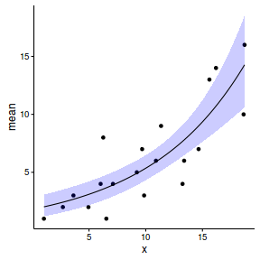
Poisson regression (count data) with overdispersion
There are numerous ways to deal with overdispersion. The traditional way was to use a 'quasi' family. Such an approach fits a regular distribution and then alters the standard errors according to the degree of overdispersion and is considered by many to be a bit of a hack.
If overdispersion is the consequence of latent (un-measured or un-modelled) influences inflating the variances, then one alternative is to incorporate a latent variable that will 'soak' up this additional variance. This is the theory behind including a unit-level random effect.
- define a function that will generate random samples from a quasi-poisson distribution $$QuasiPoisson\left(\frac{\mu}{\phi-1}, \frac{1}{\phi}\right)$$ where $\mu$ is the expected value (mean) and $\phi$ is the dispersion factor such that $var(y)=\phi\mu$.
- the sample size = 20
- the continuous $x$ variable is a random uniform spread of measurements between 1 and 20
- the rate of change in log $y$ per unit of $x$ (slope) = 0.1.
- the value of $x$ when log$y$ equals 0 (when $y$=1)
- to generate the values of $y$ expected at each $x$ value, we evaluate the linear predictor (created by calculating the outer product of the model matrix and the regression parameters). These expected values are then transformed into a scale mapped by (0,$\infty$) by using the log function $e^{linear~predictor}$
- finally, we generate $y$ values by using the expected $y$ values ($\lambda$) as probabilities when drawing random numbers from a quasi-poisson distribution. This step adds random noise to the expected $y$ values and returns only 0's and positive integers.
#Quasi-poisson distrition
rqpois <- function(n, lambda, phi) {
  mu = lambda
  r = rnbinom(n, size=mu/phi/(1-1/phi),prob=1/phi)
  return(r)
}

set.seed(8)
#The number of samples
n.x <- 20
#Create x values that at uniformly distributed throughout the rate of 1 to 20
x <- sort(runif(n = n.x, min = 1, max =20))
mm <- model.matrix(~x)
intercept <- 0.6
slope=0.1
#The linear predictor
linpred <- mm %*% c(intercept,slope)
#Predicted y values
lambda <- exp(linpred)
#Add some noise and make binomial
y <- rqpois(n=n.x, lambda=lambda, phi=4)
dat.qp <- data.frame(y,x)
data.qp <- dat.qp
$$ \begin{align} y_{ij} &\sim{} Pois(\lambda_{ij})\\ log(\lambda_{ij})&=\beta_0+\beta_1x_1 + \sum^j_{J=1} \gamma U_j\\ \end{align} $$
library(lme4)
data.qp$unit=1:nrow(data.qp)
dat.glm <- glmer(y~x+(1|unit), data=data.qp, family="poisson")
summary(dat.glm)
Generalized linear mixed model fit by maximum likelihood (Laplace Approximation) ['glmerMod']
 Family: poisson  ( log )
Formula: y ~ x + (1 | unit)
   Data: data.qp

     AIC      BIC   logLik deviance df.resid
   114.6    117.6    -54.3    108.6       17

Scaled residuals:
     Min       1Q   Median       3Q      Max
-1.37873 -0.65032  0.04504  0.41908  0.68899

Random effects:
 Groups Name        Variance Std.Dev.
 unit   (Intercept) 0.4251   0.652
Number of obs: 20, groups:  unit, 20

Fixed effects:
            Estimate Std. Error z value Pr(>|z|)
(Intercept)  0.19971    0.47627   0.419 0.674981
x            0.12684    0.03833   3.309 0.000936 ***
---
Signif. codes:  0 '***' 0.001 '**' 0.01 '*' 0.05 '.' 0.1 ' ' 1

Correlation of Fixed Effects:
  (Intr)
x -0.915
data.qp$unit=1:nrow(data.qp)
modelString="
model{
  for (i in 1:N) {
    y[i] ~ dpois(lambda[i])
    log(lambda[i]) <- max(-20,min(20,beta0+beta1*x[i] + gamma[U[i]]))
  }
  beta0 ~ dnorm(0,1.0E-06)
  beta1 ~ dnorm(0,1.0E-06)
  for (j in 1:nU) {
    gamma[j] ~ dnorm(0, tau)
  }
  ## Half-cauchy (scale=25) prior
  tau <- pow(sigma,-2)
  sigma <-z/sqrt(chSq)
  z ~ dnorm(0, .0016)I(0,)
  chSq ~ dgamma(0.5, 0.5)
}
"
dat.list <- with(data.qp, list(y=y, x=x, U=as.numeric(unit), nU=nrow(data.qp), N=nrow(data.qp)))
dat.jags <- jags(data=dat.list,model.file=textConnection(modelString),
                   param=c('beta0','beta1','sigma'),
                   n.chains=3, n.iter=20000, n.burnin=10000, n.thin=100)
Compiling model graph
   Resolving undeclared variables
   Allocating nodes
   Graph Size: 197

Initializing model
print(dat.jags)
Inference for Bugs model at "5", fit using jags,
 3 chains, each with 20000 iterations (first 10000 discarded), n.thin = 100
 n.sims = 300 iterations saved
         mu.vect sd.vect   2.5%    25%    50%    75%  97.5%  Rhat n.eff
beta0      0.001   0.651 -1.431 -0.362  0.075  0.421  1.201 1.047    60
beta1      0.141   0.053  0.046  0.110  0.137  0.172  0.250 1.049    67
sigma      0.852   0.284  0.456  0.666  0.802  0.965  1.576 1.006   210
deviance  84.483   6.824 74.009 79.661 84.080 88.029 98.306 0.997   300

For each parameter, n.eff is a crude measure of effective sample size,
and Rhat is the potential scale reduction factor (at convergence, Rhat=1).

DIC info (using the rule, pD = var(deviance)/2)
pD = 23.4 and DIC = 107.9
DIC is an estimate of expected predictive error (lower deviance is better).
data.qp$unit=1:nrow(data.qp)
library(rstan)
modelString="
data {
   int<lower=1> n;
   int<lower=1> nX;
   int<lower=1> nU;
   int y[n];
   matrix [n,nX] X;
   int U[n];
}
parameters {
   vector [nX] beta;
   vector [nU] gamma;
   real<lower=0> sigma;
}
transformed parameters {
   vector [n] mu;
   mu<-X*beta;
   for (i in 1:n) {
     mu[i] <- mu[i] + gamma[U[i]];
   }
}
model {
   beta ~ normal(0,1000);
   sigma ~ cauchy(0,25);
   gamma ~ normal(0,sigma);

   y ~ poisson_log(mu);
}
"
Xmat <- model.matrix(~x,data=data.qp)
dat.list <- with(data.qp, list(y = y, X = Xmat, nX=ncol(Xmat),
                 U=as.numeric(unit), nU=nrow(data.qp),
                 n = nrow(data.qp)))

library(rstan)
dat.rstan <- stan(data=dat.list,
           model_code=modelString,
           chains=3,
           iter=1000,
           warmup=500,
                   thin=2,
           save_dso=TRUE
           )
SAMPLING FOR MODEL '6b01137f7762e83c8564fa8b7bbd08b8' NOW (CHAIN 1).

Chain 1, Iteration:   1 / 1000 [  0%]  (Warmup)
Chain 1, Iteration: 100 / 1000 [ 10%]  (Warmup)
Chain 1, Iteration: 200 / 1000 [ 20%]  (Warmup)
Chain 1, Iteration: 300 / 1000 [ 30%]  (Warmup)
Chain 1, Iteration: 400 / 1000 [ 40%]  (Warmup)
Chain 1, Iteration: 500 / 1000 [ 50%]  (Warmup)
Chain 1, Iteration: 501 / 1000 [ 50%]  (Sampling)
Chain 1, Iteration: 600 / 1000 [ 60%]  (Sampling)
Chain 1, Iteration: 700 / 1000 [ 70%]  (Sampling)
Chain 1, Iteration: 800 / 1000 [ 80%]  (Sampling)
Chain 1, Iteration: 900 / 1000 [ 90%]  (Sampling)
Chain 1, Iteration: 1000 / 1000 [100%]  (Sampling)#
#  Elapsed Time: 0.291649 seconds (Warm-up)
#                0.151107 seconds (Sampling)
#                0.442756 seconds (Total)
#

SAMPLING FOR MODEL '6b01137f7762e83c8564fa8b7bbd08b8' NOW (CHAIN 2).

Chain 2, Iteration:   1 / 1000 [  0%]  (Warmup)
Chain 2, Iteration: 100 / 1000 [ 10%]  (Warmup)
Chain 2, Iteration: 200 / 1000 [ 20%]  (Warmup)
Chain 2, Iteration: 300 / 1000 [ 30%]  (Warmup)
Chain 2, Iteration: 400 / 1000 [ 40%]  (Warmup)
Chain 2, Iteration: 500 / 1000 [ 50%]  (Warmup)
Chain 2, Iteration: 501 / 1000 [ 50%]  (Sampling)
Chain 2, Iteration: 600 / 1000 [ 60%]  (Sampling)
Chain 2, Iteration: 700 / 1000 [ 70%]  (Sampling)
Chain 2, Iteration: 800 / 1000 [ 80%]  (Sampling)
Chain 2, Iteration: 900 / 1000 [ 90%]  (Sampling)
Chain 2, Iteration: 1000 / 1000 [100%]  (Sampling)#
#  Elapsed Time: 0.279321 seconds (Warm-up)
#                0.102494 seconds (Sampling)
#                0.381815 seconds (Total)
#

SAMPLING FOR MODEL '6b01137f7762e83c8564fa8b7bbd08b8' NOW (CHAIN 3).

Chain 3, Iteration:   1 / 1000 [  0%]  (Warmup)
Chain 3, Iteration: 100 / 1000 [ 10%]  (Warmup)
Chain 3, Iteration: 200 / 1000 [ 20%]  (Warmup)
Chain 3, Iteration: 300 / 1000 [ 30%]  (Warmup)
Chain 3, Iteration: 400 / 1000 [ 40%]  (Warmup)
Chain 3, Iteration: 500 / 1000 [ 50%]  (Warmup)
Chain 3, Iteration: 501 / 1000 [ 50%]  (Sampling)
Chain 3, Iteration: 600 / 1000 [ 60%]  (Sampling)
Chain 3, Iteration: 700 / 1000 [ 70%]  (Sampling)
Chain 3, Iteration: 800 / 1000 [ 80%]  (Sampling)
Chain 3, Iteration: 900 / 1000 [ 90%]  (Sampling)
Chain 3, Iteration: 1000 / 1000 [100%]  (Sampling)#
#  Elapsed Time: 0.306079 seconds (Warm-up)
#                0.110866 seconds (Sampling)
#                0.416945 seconds (Total)
#
print(dat.rstan, pars=c('beta','sigma'))
Inference for Stan model: 6b01137f7762e83c8564fa8b7bbd08b8.
3 chains, each with iter=1000; warmup=500; thin=2;
post-warmup draws per chain=250, total post-warmup draws=750.

        mean se_mean   sd  2.5%   25%  50%  75% 97.5% n_eff Rhat
beta[1] 0.01    0.03 0.59 -1.25 -0.36 0.06 0.42  1.01   314 1.00
beta[2] 0.14    0.00 0.05  0.05  0.11 0.13 0.17  0.23   287 1.00
sigma   0.85    0.02 0.26  0.47  0.67 0.81 0.98  1.44   248 1.01

Samples were drawn using NUTS(diag_e) at Tue Feb 23 12:30:49 2016.
For each parameter, n_eff is a crude measure of effective sample size,
and Rhat is the potential scale reduction factor on split chains (at
convergence, Rhat=1).
data.qp$unit=1:nrow(data.qp)
library(brms)
dat.brm <- brm(y~x+(1|unit), data=data.qp, family='poisson',
   prior=c(set_prior('normal(0,1000)', class='b')),
   chains=3, iter=1000, warmup=500, thin=2
)
SAMPLING FOR MODEL 'poisson(log) brms-model' NOW (CHAIN 1).

Chain 1, Iteration:   1 / 1000 [  0%]  (Warmup)
Chain 1, Iteration: 100 / 1000 [ 10%]  (Warmup)
Chain 1, Iteration: 200 / 1000 [ 20%]  (Warmup)
Chain 1, Iteration: 300 / 1000 [ 30%]  (Warmup)
Chain 1, Iteration: 400 / 1000 [ 40%]  (Warmup)
Chain 1, Iteration: 500 / 1000 [ 50%]  (Warmup)
Chain 1, Iteration: 501 / 1000 [ 50%]  (Sampling)
Chain 1, Iteration: 600 / 1000 [ 60%]  (Sampling)
Chain 1, Iteration: 700 / 1000 [ 70%]  (Sampling)
Chain 1, Iteration: 800 / 1000 [ 80%]  (Sampling)
Chain 1, Iteration: 900 / 1000 [ 90%]  (Sampling)
Chain 1, Iteration: 1000 / 1000 [100%]  (Sampling)#
#  Elapsed Time: 0.139169 seconds (Warm-up)
#                0.059387 seconds (Sampling)
#                0.198556 seconds (Total)
#

SAMPLING FOR MODEL 'poisson(log) brms-model' NOW (CHAIN 2).

Chain 2, Iteration:   1 / 1000 [  0%]  (Warmup)
Chain 2, Iteration: 100 / 1000 [ 10%]  (Warmup)
Chain 2, Iteration: 200 / 1000 [ 20%]  (Warmup)
Chain 2, Iteration: 300 / 1000 [ 30%]  (Warmup)
Chain 2, Iteration: 400 / 1000 [ 40%]  (Warmup)
Chain 2, Iteration: 500 / 1000 [ 50%]  (Warmup)
Chain 2, Iteration: 501 / 1000 [ 50%]  (Sampling)
Chain 2, Iteration: 600 / 1000 [ 60%]  (Sampling)
Chain 2, Iteration: 700 / 1000 [ 70%]  (Sampling)
Chain 2, Iteration: 800 / 1000 [ 80%]  (Sampling)
Chain 2, Iteration: 900 / 1000 [ 90%]  (Sampling)
Chain 2, Iteration: 1000 / 1000 [100%]  (Sampling)#
#  Elapsed Time: 0.165589 seconds (Warm-up)
#                0.062659 seconds (Sampling)
#                0.228248 seconds (Total)
#

SAMPLING FOR MODEL 'poisson(log) brms-model' NOW (CHAIN 3).

Chain 3, Iteration:   1 / 1000 [  0%]  (Warmup)
Chain 3, Iteration: 100 / 1000 [ 10%]  (Warmup)
Chain 3, Iteration: 200 / 1000 [ 20%]  (Warmup)
Chain 3, Iteration: 300 / 1000 [ 30%]  (Warmup)
Chain 3, Iteration: 400 / 1000 [ 40%]  (Warmup)
Chain 3, Iteration: 500 / 1000 [ 50%]  (Warmup)
Chain 3, Iteration: 501 / 1000 [ 50%]  (Sampling)
Chain 3, Iteration: 600 / 1000 [ 60%]  (Sampling)
Chain 3, Iteration: 700 / 1000 [ 70%]  (Sampling)
Chain 3, Iteration: 800 / 1000 [ 80%]  (Sampling)
Chain 3, Iteration: 900 / 1000 [ 90%]  (Sampling)
Chain 3, Iteration: 1000 / 1000 [100%]  (Sampling)#
#  Elapsed Time: 0.140647 seconds (Warm-up)
#                0.056132 seconds (Sampling)
#                0.196779 seconds (Total)
#
summary(dat.brm)
 Family: poisson (log)
Formula: y ~ x + (1 | unit)
   Data: data.qp (Number of observations: 20)
Samples: 3 chains, each with iter = 1000; warmup = 500; thin = 2;
         total post-warmup samples = 750
   WAIC: Not computed

Random Effects:
~unit (Number of levels: 20)
              Estimate Est.Error l-95% CI u-95% CI Eff.Sample Rhat
sd(Intercept)     0.83      0.26     0.46     1.43        171 1.01

Fixed Effects:
          Estimate Est.Error l-95% CI u-95% CI Eff.Sample Rhat
Intercept     0.07      0.55    -1.04     1.14        480    1
x             0.13      0.05     0.05     0.23        348    1

Samples were drawn using sampling(NUTS). For each parameter, Eff.Sample
is a crude measure of effective sample size, and Rhat is the potential
scale reduction factor on split chains (at convergence, Rhat = 1).
stancode(dat.brm)
functions {
}
data {
  int<lower=1> N;  // number of observations
  int Y[N];  // response variable
  int<lower=1> K;  // number of fixed effects
  matrix[N, K] X;  // FE design matrix
  vector[K] X_means;  // column means of X
  // data for random effects of unit
  int<lower=1> J_1[N];  // RE levels
  int<lower=1> N_1;  // number of levels
  int<lower=1> K_1;  // number of REs
  real Z_1[N];  // RE design matrix
}
transformed data {
}
parameters {
  real temp_Intercept;  // temporary Intercept
  vector[K] b;  // fixed effects
  vector[N_1] pre_1;  // unscaled REs
  real<lower=0> sd_1;  // RE standard deviation
}
transformed parameters {
  vector[N] eta;  // linear predictor
  vector[N_1] r_1;  // REs
  // compute linear predictor
  eta <- X * b + temp_Intercept;
  r_1 <- sd_1 * (pre_1);  // scale REs
  for (n in 1:N) {
    eta[n] <- eta[n] + Z_1[n] * r_1[J_1[n]];
  }
}
model {
  // prior specifications
  b ~ normal(0,1000);
  sd_1 ~ student_t(3, 0, 5);
  pre_1 ~ normal(0, 1);
  // likelihood contribution
  Y ~ poisson_log(eta);
}
generated quantities {
  real b_Intercept;  // fixed effects intercept
  b_Intercept <- temp_Intercept - dot_product(X_means, b);
}
fitted <- subset(data.qp, select=c(x,y, unit))
fitted$y <- NA
newdata <- expand.grid(x=seq(min(data.qp$x), max(data.qp$x), len=100), y=NA, unit=NA)
dat.pred <- rbind(data.qp,fitted,newdata)
Now lets fit the model.
#fit the model
dat.inla <- inla(y~x+f(unit, model='iid'), family='poisson',
   data=dat.pred,
   control.family=list(link='log'),
   control.predictor=list(link=1, compute=TRUE),
   control.compute=list(dic=TRUE, cpo=TRUE, waic=TRUE))
#examine the regular summary
summary(dat.inla)
Call:
c("inla(formula = y ~ x + f(unit, model = \"iid\"), family = \"poisson\", ",  "    data = dat.pred, control.compute = list(dic = TRUE, cpo = TRUE, ",  "        waic = TRUE), control.predictor = list(link = 1, compute = TRUE), ",  "    control.family = list(link = \"log\"))")

Time used:
 Pre-processing    Running inla Post-processing           Total
         0.0950          0.0728          0.0331          0.2008

Fixed effects:
              mean     sd 0.025quant 0.5quant 0.975quant   mode kld
(Intercept) 0.2176 0.4647    -0.7614   0.2394     1.0738 0.2822   0
x           0.1263 0.0378     0.0549   0.1251     0.2046 0.1229   0

Random effects:
Name	  Model
 unit   IID model

Model hyperparameters:
                    mean    sd 0.025quant 0.5quant 0.975quant  mode
Precision for unit 3.154 2.022     0.8659    2.647      8.429 1.889

Expected number of effective parameters(std dev): 13.15(1.516)
Number of equivalent replicates : 1.521

Deviance Information Criterion (DIC) ...: 100.91
Effective number of parameters .........: 13.48

Watanabe-Akaike information criterion (WAIC) ...: 100.97
Effective number of parameters .................: 10.12

Marginal log-Likelihood:  -70.59
CPO and PIT are computed

Posterior marginals for linear predictor and fitted values computed
newdata <- cbind(newdata,
  dat.inla$summary.fitted.values[(nrow(data.qp)+nrow(fitted)+1):nrow(dat.pred),])
head(newdata)
x y unit mean sd 0.025quant 0.5quant 0.975quant mode fitted.predictor.041 1.024733 NA NA 1.546157 0.6600472 0.5723928 1.443850 3.115993 1.263051 fitted.predictor.042 1.203403 NA NA 1.577515 0.6633672 0.5928836 1.476424 3.151031 1.297411 fitted.predictor.043 1.382074 NA NA 1.609575 0.6666484 0.6140817 1.509731 3.186584 1.332625 fitted.predictor.044 1.560745 NA NA 1.642354 0.6698890 0.6360093 1.543786 3.222667 1.368681 fitted.predictor.045 1.739415 NA NA 1.675869 0.6730872 0.6586892 1.578607 3.259294 1.405544 fitted.predictor.046 1.918086 NA NA 1.710138 0.6762414 0.6821445 1.614211 3.296481 1.443231
newdata <- reshape:::rename(newdata, c("0.025quant"="lower", "0.975quant"="upper")) library(grid) ggplot(newdata, aes(y=mean, x=x)) + geom_blank()+ geom_point(data=data.qp, aes(y=y, x=x)) + geom_ribbon(aes(ymin=lower, ymax=upper), fill='blue', alpha=0.2) + geom_line() + theme_classic()+ theme(legend.key.width=unit(2,'lines'), legend.position=c(0,1), legend.justification=c(0,1))
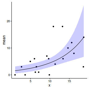
Negative Binomial regression (overdispersed count data)
The Negative Binomial distribution strictly represents the number of successes before a failure. In practice it is a beta-poisson distribution. As such, it is a distribution that is defined by two parameters (which can be defined in terms of location and scale). When the model has a dispersion parameter of 1 (when $\lambda = \mu = \sigma^2$), the Negative Binomial distribution is equivalent to a Poisson distribution.
Hence rather than assume that the dispersion parameter is 1 ($\lambda = \mu = \sigma^2$), we can use a distribution that estimates the scale as well as the location parameter.
- the sample size = 20
- the continuous $x$ variable is a random uniform spread of measurements between 1 and 20
- the rate of change in log $y$ per unit of $x$ (slope) = 0.1.
- the value of $x$ when log$y$ equals 0 (when $y$=1)
- to generate the values of $y$ expected at each $x$ value, we evaluate the linear predictor (created by calculating the outer product of the model matrix and the regression parameters). These expected values are then transformed into a scale mapped by (0,$\infty$) by using the log function $e^{linear~predictor}$
- finally, we generate $y$ values by using the expected $y$ values ($\lambda$) as probabilities when drawing random numbers from a Poisson distribution. This step adds random noise to the expected $y$ values and returns only 0's and positive integers.
set.seed(37) #16 #35 #The number of samples n.x <- 20 #Create x values that at uniformly distributed throughout the rate of 1 to 20 x <- sort(runif(n = n.x, min = 1, max =20)) mm <- model.matrix(~x) intercept <- 0.6 slope=0.1 #The linear predictor linpred <- mm %*% c(intercept,slope) #Predicted y values lambda <- exp(linpred) #Add some noise and make binomial y <- rnbinom(n=n.x, mu=lambda, size=1) dat.nb <- data.frame(y,x) data.nb <- dat.nb
$$ \begin{align} y_{ij} &\sim{} NB(p_{ij}, size)\\ p_{ij} &= size/(size+\lambda_{ij})\\ log(\lambda_{ij})&=\beta_0+\beta_1x_1 + \sum^j_{J=1} \gamma U_j\\ size &\sim{} U(0.001, 10000)\\ \end{align} $$
library(MASS) dat.glm <- glm.nb(y~x, data=data.nb) summary(dat.glm)
Call:
glm.nb(formula = y ~ x, data = data.nb, init.theta = 2.359878187,
link = log)
Deviance Residuals:
Min 1Q Median 3Q Max
-2.7874 -0.8940 -0.3172 0.4420 1.3660
Coefficients:
Estimate Std. Error z value Pr(>|z|)
(Intercept) 0.74543 0.42534 1.753 0.07968 .
x 0.09494 0.03441 2.759 0.00579 **
---
Signif. codes: 0 '***' 0.001 '**' 0.01 '*' 0.05 '.' 0.1 ' ' 1
(Dispersion parameter for Negative Binomial(2.3599) family taken to be 1)
Null deviance: 30.443 on 19 degrees of freedom
Residual deviance: 21.806 on 18 degrees of freedom
AIC: 115.85
Number of Fisher Scoring iterations: 1
Theta: 2.36
Std. Err.: 1.10
2 x log-likelihood: -109.849
data.qp$unit=1:nrow(data.qp) modelString=" model{ for (i in 1:N) { y[i] ~ dnegbin(p[i],size) p[i] <- size/(size+lambda[i]) log(lambda[i]) <- max(-20,min(20,beta0+beta1*x[i])) } beta0 ~ dnorm(0,1.0E-06) beta1 ~ dnorm(0,1.0E-06) size ~ dunif(0.001, 1000) } " dat.list <- with(data.nb, list(y=y, x=x, N=nrow(data.nb))) dat.jags <- jags(data=dat.list,model.file=textConnection(modelString), param=c('beta0','beta1','size'), n.chains=3, n.iter=20000, n.burnin=10000, n.thin=100)
Compiling model graph Resolving undeclared variables Allocating nodes Graph Size: 190 Initializing model
print(dat.jags)
Inference for Bugs model at "5", fit using jags,
3 chains, each with 20000 iterations (first 10000 discarded), n.thin = 100
n.sims = 300 iterations saved
mu.vect sd.vect 2.5% 25% 50% 75% 97.5% Rhat n.eff
beta0 0.761 0.425 0.014 0.471 0.732 1.014 1.616 0.997 300
beta1 0.094 0.033 0.022 0.073 0.095 0.117 0.150 0.999 300
size 3.916 7.867 1.038 2.034 2.742 3.766 8.598 1.060 160
deviance 113.293 3.196 110.049 111.142 112.441 114.103 121.912 1.043 160
For each parameter, n.eff is a crude measure of effective sample size,
and Rhat is the potential scale reduction factor (at convergence, Rhat=1).
DIC info (using the rule, pD = var(deviance)/2)
pD = 5.1 and DIC = 118.4
DIC is an estimate of expected predictive error (lower deviance is better).
library(rstan) modelString=" data { int<lower=1> n; int<lower=1> nX; int y[n]; matrix [n,nX] X; } parameters { vector [nX] beta; real<lower=0> shape; } transformed parameters { vector [n] eta; eta<-X*beta; } model { beta ~ normal(0,1000); shape ~ student_t(3,0,5); y ~ neg_binomial_2_log(eta, shape); } " Xmat <- model.matrix(~x,data=data.nb) dat.list <- with(data.nb, list(y = y, X = Xmat, nX=ncol(Xmat), n = nrow(data.nb))) library(rstan) dat.rstan <- stan(data=dat.list, model_code=modelString, chains=3, iter=1000, warmup=500, thin=2, save_dso=TRUE )
SAMPLING FOR MODEL '7ed6b7a1636f285e8c38d5fd272fc919' NOW (CHAIN 1). Chain 1, Iteration: 1 / 1000 [ 0%] (Warmup) Chain 1, Iteration: 100 / 1000 [ 10%] (Warmup) Chain 1, Iteration: 200 / 1000 [ 20%] (Warmup) Chain 1, Iteration: 300 / 1000 [ 30%] (Warmup) Chain 1, Iteration: 400 / 1000 [ 40%] (Warmup) Chain 1, Iteration: 500 / 1000 [ 50%] (Warmup) Chain 1, Iteration: 501 / 1000 [ 50%] (Sampling) Chain 1, Iteration: 600 / 1000 [ 60%] (Sampling) Chain 1, Iteration: 700 / 1000 [ 70%] (Sampling) Chain 1, Iteration: 800 / 1000 [ 80%] (Sampling) Chain 1, Iteration: 900 / 1000 [ 90%] (Sampling) Chain 1, Iteration: 1000 / 1000 [100%] (Sampling)# # Elapsed Time: 3.8897 seconds (Warm-up) # 0.22708 seconds (Sampling) # 4.11678 seconds (Total) # SAMPLING FOR MODEL '7ed6b7a1636f285e8c38d5fd272fc919' NOW (CHAIN 2). Chain 2, Iteration: 1 / 1000 [ 0%] (Warmup) Chain 2, Iteration: 100 / 1000 [ 10%] (Warmup) Chain 2, Iteration: 200 / 1000 [ 20%] (Warmup) Chain 2, Iteration: 300 / 1000 [ 30%] (Warmup) Chain 2, Iteration: 400 / 1000 [ 40%] (Warmup) Chain 2, Iteration: 500 / 1000 [ 50%] (Warmup) Chain 2, Iteration: 501 / 1000 [ 50%] (Sampling) Chain 2, Iteration: 600 / 1000 [ 60%] (Sampling) Chain 2, Iteration: 700 / 1000 [ 70%] (Sampling) Chain 2, Iteration: 800 / 1000 [ 80%] (Sampling) Chain 2, Iteration: 900 / 1000 [ 90%] (Sampling) Chain 2, Iteration: 1000 / 1000 [100%] (Sampling)# # Elapsed Time: 6.20803 seconds (Warm-up) # 12.3776 seconds (Sampling) # 18.5856 seconds (Total) # SAMPLING FOR MODEL '7ed6b7a1636f285e8c38d5fd272fc919' NOW (CHAIN 3). Chain 3, Iteration: 1 / 1000 [ 0%] (Warmup) Chain 3, Iteration: 100 / 1000 [ 10%] (Warmup) Chain 3, Iteration: 200 / 1000 [ 20%] (Warmup) Chain 3, Iteration: 300 / 1000 [ 30%] (Warmup) Chain 3, Iteration: 400 / 1000 [ 40%] (Warmup) Chain 3, Iteration: 500 / 1000 [ 50%] (Warmup) Chain 3, Iteration: 501 / 1000 [ 50%] (Sampling) Chain 3, Iteration: 600 / 1000 [ 60%] (Sampling) Chain 3, Iteration: 700 / 1000 [ 70%] (Sampling) Chain 3, Iteration: 800 / 1000 [ 80%] (Sampling) Chain 3, Iteration: 900 / 1000 [ 90%] (Sampling) Chain 3, Iteration: 1000 / 1000 [100%] (Sampling)# # Elapsed Time: 3.37625 seconds (Warm-up) # 0.126583 seconds (Sampling) # 3.50283 seconds (Total) #
print(dat.rstan, pars=c('beta','shape'))
Inference for Stan model: 7ed6b7a1636f285e8c38d5fd272fc919.
3 chains, each with iter=1000; warmup=500; thin=2;
post-warmup draws per chain=250, total post-warmup draws=750.
mean se_mean sd 2.5% 25% 50% 75% 97.5% n_eff Rhat
beta[1] 0.57 0.21 0.56 -0.40 0.15 0.60 0.97 1.74 7 1.31
beta[2] 0.11 0.01 0.04 0.03 0.08 0.10 0.13 0.18 11 1.25
shape 1.57 0.05 0.31 0.87 1.37 1.59 1.84 1.98 43 1.08
Samples were drawn using NUTS(diag_e) at Tue Feb 23 16:08:26 2016.
For each parameter, n_eff is a crude measure of effective sample size,
and Rhat is the potential scale reduction factor on split chains (at
convergence, Rhat=1).
library(brms) dat.brm <- brm(y~x, data=data.nb, family='negbinomial', prior=c(set_prior('normal(0,1000)', class='b')), chains=3, iter=1000, warmup=500, thin=2 )
SAMPLING FOR MODEL 'negbinomial(log) brms-model' NOW (CHAIN 1). Chain 1, Iteration: 1 / 1000 [ 0%] (Warmup) Chain 1, Iteration: 100 / 1000 [ 10%] (Warmup) Chain 1, Iteration: 200 / 1000 [ 20%] (Warmup) Chain 1, Iteration: 300 / 1000 [ 30%] (Warmup) Chain 1, Iteration: 400 / 1000 [ 40%] (Warmup) Chain 1, Iteration: 500 / 1000 [ 50%] (Warmup) Chain 1, Iteration: 501 / 1000 [ 50%] (Sampling) Chain 1, Iteration: 600 / 1000 [ 60%] (Sampling) Chain 1, Iteration: 700 / 1000 [ 70%] (Sampling) Chain 1, Iteration: 800 / 1000 [ 80%] (Sampling) Chain 1, Iteration: 900 / 1000 [ 90%] (Sampling) Chain 1, Iteration: 1000 / 1000 [100%] (Sampling)# # Elapsed Time: 3.63316 seconds (Warm-up) # 12.482 seconds (Sampling) # 16.1151 seconds (Total) # SAMPLING FOR MODEL 'negbinomial(log) brms-model' NOW (CHAIN 2). Chain 2, Iteration: 1 / 1000 [ 0%] (Warmup) Chain 2, Iteration: 100 / 1000 [ 10%] (Warmup) Chain 2, Iteration: 200 / 1000 [ 20%] (Warmup) Chain 2, Iteration: 300 / 1000 [ 30%] (Warmup) Chain 2, Iteration: 400 / 1000 [ 40%] (Warmup) Chain 2, Iteration: 500 / 1000 [ 50%] (Warmup) Chain 2, Iteration: 501 / 1000 [ 50%] (Sampling) Chain 2, Iteration: 600 / 1000 [ 60%] (Sampling) Chain 2, Iteration: 700 / 1000 [ 70%] (Sampling) Chain 2, Iteration: 800 / 1000 [ 80%] (Sampling) Chain 2, Iteration: 900 / 1000 [ 90%] (Sampling) Chain 2, Iteration: 1000 / 1000 [100%] (Sampling)# # Elapsed Time: 7.01036 seconds (Warm-up) # 12.4126 seconds (Sampling) # 19.423 seconds (Total) # SAMPLING FOR MODEL 'negbinomial(log) brms-model' NOW (CHAIN 3). Chain 3, Iteration: 1 / 1000 [ 0%] (Warmup) Chain 3, Iteration: 100 / 1000 [ 10%] (Warmup) Chain 3, Iteration: 200 / 1000 [ 20%] (Warmup) Chain 3, Iteration: 300 / 1000 [ 30%] (Warmup) Chain 3, Iteration: 400 / 1000 [ 40%] (Warmup) Chain 3, Iteration: 500 / 1000 [ 50%] (Warmup) Chain 3, Iteration: 501 / 1000 [ 50%] (Sampling) Chain 3, Iteration: 600 / 1000 [ 60%] (Sampling) Chain 3, Iteration: 700 / 1000 [ 70%] (Sampling) Chain 3, Iteration: 800 / 1000 [ 80%] (Sampling) Chain 3, Iteration: 900 / 1000 [ 90%] (Sampling) Chain 3, Iteration: 1000 / 1000 [100%] (Sampling)# # Elapsed Time: 5.72697 seconds (Warm-up) # 4.75621 seconds (Sampling) # 10.4832 seconds (Total) #
summary(dat.brm)
Family: negbinomial (log)
Formula: y ~ x
Data: data.nb (Number of observations: 20)
Samples: 3 chains, each with iter = 1000; warmup = 500; thin = 2;
total post-warmup samples = 750
WAIC: Not computed
Fixed Effects:
Estimate Est.Error l-95% CI u-95% CI Eff.Sample Rhat
Intercept 0.79 0.48 -0.04 1.91 80 1.02
x 0.09 0.04 0.01 0.17 104 1.01
Family Specific Parameters:
Estimate Est.Error l-95% CI u-95% CI Eff.Sample Rhat
shape 1.57 0.29 0.91 1.98 89 1.01
Samples were drawn using sampling(NUTS). For each parameter, Eff.Sample
is a crude measure of effective sample size, and Rhat is the potential
scale reduction factor on split chains (at convergence, Rhat = 1).
stancode(dat.brm)
functions {
}
data {
int<lower=1> N; // number of observations
int Y[N]; // response variable
int<lower=1> K; // number of fixed effects
matrix[N, K] X; // FE design matrix
vector[K] X_means; // column means of X
}
transformed data {
}
parameters {
real temp_Intercept; // temporary Intercept
vector[K] b; // fixed effects
real<lower=0> shape; // shape parameter
}
transformed parameters {
vector[N] eta; // linear predictor
// compute linear predictor
eta <- X * b + temp_Intercept;
}
model {
// prior specifications
b ~ normal(0,1000);
shape ~ student_t(3, 0, 5);
// likelihood contribution
Y ~ neg_binomial_2_log(eta, shape);
}
generated quantities {
real b_Intercept; // fixed effects intercept
b_Intercept <- temp_Intercept - dot_product(X_means, b);
}
fitted <- subset(data.nb, select=c(x,y)) fitted$y <- NA newdata <- expand.grid(x=seq(min(data.nb$x), max(data.nb$x), len=100), y=NA) dat.pred <- rbind(data.nb,fitted,newdata)
Now lets fit the model.
#fit the model dat.inla <- inla(y~x, family='nbinomial', data=dat.pred, control.family=list(link='log'), control.predictor=list(link=1, compute=TRUE), control.compute=list(dic=TRUE, cpo=TRUE, waic=TRUE)) #examine the regular summary summary(dat.inla)
Call:
c("inla(formula = y ~ x, family = \"nbinomial\", data = dat.pred, ", " control.compute = list(dic = TRUE, cpo = TRUE, waic = TRUE), ", " control.predictor = list(link = 1, compute = TRUE), control.family = list(link = \"log\"))" )
Time used:
Pre-processing Running inla Post-processing Total
0.0866 0.0483 0.0302 0.1650
Fixed effects:
mean sd 0.025quant 0.5quant 0.975quant mode kld
(Intercept) 0.7439 0.4569 -0.1380 0.7379 1.6633 0.7283 0
x 0.0949 0.0368 0.0226 0.0948 0.1680 0.0944 0
The model has no random effects
Model hyperparameters:
mean sd 0.025quant 0.5quant 0.975quant mode
size for the nbinomial observations (overdispersion) 1.859 0.7529 0.794 1.725 3.702 1.485
Expected number of effective parameters(std dev): 2.00(1e-04)
Number of equivalent replicates : 9.998
Deviance Information Criterion (DIC) ...: 115.27
Effective number of parameters .........: 2.474
Watanabe-Akaike information criterion (WAIC) ...: 115.09
Effective number of parameters .................: 2.055
Marginal log-Likelihood: -63.84
CPO and PIT are computed
Posterior marginals for linear predictor and fitted values computed
newdata <- cbind(newdata, dat.inla$summary.fitted.values[(nrow(data.nb)+nrow(fitted)+1):nrow(dat.pred),]) head(newdata)
x y mean sd 0.025quant 0.5quant 0.975quant mode fitted.predictor.041 1.042191 NA 2.546251 1.166255 1.029584 2.311028 5.447691 1.940691 fitted.predictor.042 1.217094 NA 2.582946 1.165233 1.058728 2.350080 5.477622 1.982258 fitted.predictor.043 1.391996 NA 2.620294 1.164145 1.088655 2.389805 5.507934 2.024570 fitted.predictor.044 1.566899 NA 2.658306 1.162991 1.119382 2.430214 5.538646 2.067639 fitted.predictor.045 1.741802 NA 2.696996 1.161771 1.150928 2.471320 5.569776 2.111475 fitted.predictor.046 1.916705 NA 2.736379 1.160484 1.183221 2.513135 5.601344 2.156089
newdata <- reshape:::rename(newdata, c("0.025quant"="lower", "0.975quant"="upper")) library(grid) ggplot(newdata, aes(y=mean, x=x)) + geom_blank()+ geom_point(data=data.nb, aes(y=y, x=x)) + geom_ribbon(aes(ymin=lower, ymax=upper), fill='blue', alpha=0.2) + geom_line() + theme_classic()+ theme(legend.key.width=unit(2,'lines'), legend.position=c(0,1), legend.justification=c(0,1))
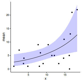
Zero-inflation Poisson (ZIP) regression (count data)
Lets say we wanted to model the abundance of an item ($y$) against a continuous predictor ($x$). As this section is mainly about the generation of artificial data (and not specifically about what to do with the data), understanding the actual details are optional and can be safely skipped. Consequently, I have folded (toggled) this section away.
- the sample size = 20
- the continuous $x$ variable is a random uniform spread of measurements between 1 and 20
- the rate of change in log $y$ per unit of $x$ (slope) = 0.1.
- the value of $x$ when log$y$ equals 0 (when $y$=1)
- to generate the values of $y$ expected at each $x$ value, we evaluate the linear predictor (created by calculating the outer product of the model matrix and the regression parameters). These expected values are then transformed into a scale mapped by (0,$\infty$) by using the log function $e^{linear~predictor}$
- finally, we generate $y$ values by using the expected $y$ values ($\lambda$) as probabilities when drawing random numbers from a Poisson distribution. This step adds random noise to the expected $y$ values and returns only 0's and positive integers.
set.seed(37) #34.5 #4 #10 #16 #17 #26 #The number of samples n.x <- 20 #Create x values that at uniformly distributed throughout the rate of 1 to 20 x <- sort(runif(n = n.x, min = 1, max =20)) mm <- model.matrix(~x) intercept <- 0.6 slope=0.1 #The linear predictor linpred <- mm %*% c(intercept,slope) #Predicted y values lambda <- exp(linpred) #Add some noise and make binomial library(gamlss.dist) #fixed latent binomial y<- rZIP(n.x,lambda, 0.4) #latent binomial influenced by the linear predictor #y<- rZIP(n.x,lambda, 1-exp(linpred)/(1+exp(linpred))) dat.zip <- data.frame(y,x) data.zip <- dat.zip summary(glm(y~x, dat.zip, family="poisson"))
Call:
glm(formula = y ~ x, family = "poisson", data = dat.zip)
Deviance Residuals:
Min 1Q Median 3Q Max
-2.5415 -2.3769 -0.9753 1.1736 3.6380
Coefficients:
Estimate Std. Error z value Pr(>|z|)
(Intercept) 0.67048 0.33018 2.031 0.0423 *
x 0.02961 0.02663 1.112 0.2662
---
Signif. codes: 0 '***' 0.001 '**' 0.01 '*' 0.05 '.' 0.1 ' ' 1
(Dispersion parameter for poisson family taken to be 1)
Null deviance: 85.469 on 19 degrees of freedom
Residual deviance: 84.209 on 18 degrees of freedom
AIC: 124.01
Number of Fisher Scoring iterations: 6
plot(glm(y~x, dat.zip, family="poisson"))
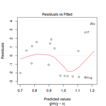
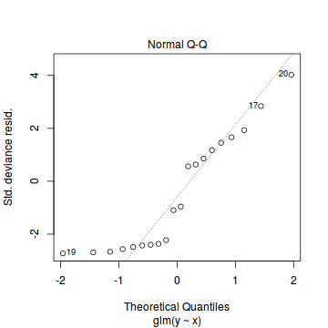
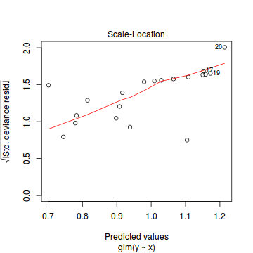
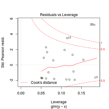
library(pscl) summary(zeroinfl(y ~ x | 1, dist = "poisson", data = dat.zip))
Call:
zeroinfl(formula = y ~ x | 1, data = dat.zip, dist = "poisson")
Pearson residuals:
Min 1Q Median 3Q Max
-1.0015 -0.9556 -0.3932 0.9663 1.6195
Count model coefficients (poisson with log link):
Estimate Std. Error z value Pr(>|z|)
(Intercept) 0.70474 0.31960 2.205 0.027449 *
x 0.08734 0.02532 3.449 0.000563 ***
Zero-inflation model coefficients (binomial with logit link):
Estimate Std. Error z value Pr(>|z|)
(Intercept) -0.2292 0.4563 -0.502 0.615
---
Signif. codes: 0 '***' 0.001 '**' 0.01 '*' 0.05 '.' 0.1 ' ' 1
Number of iterations in BFGS optimization: 13
Log-likelihood: -36.17 on 3 Df
plot(resid(zeroinfl(y ~ x | 1, dist = "poisson", data = dat.zip))~fitted(zeroinfl(y ~ x | 1, dist = "poisson", data = dat.zip)))
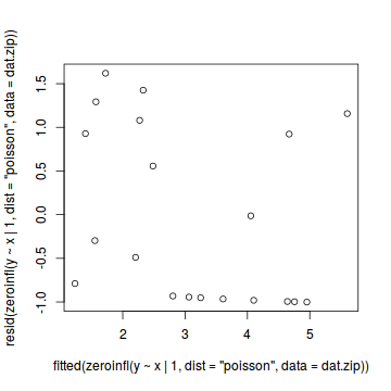
library(gamlss) summary(gamlss(y~x,data=dat.zip, family=ZIP))
GAMLSS-RS iteration 1: Global Deviance = 72.4363
GAMLSS-RS iteration 2: Global Deviance = 72.3428
GAMLSS-RS iteration 3: Global Deviance = 72.3428
*******************************************************************
Family: c("ZIP", "Poisson Zero Inflated")
Call: gamlss(formula = y ~ x, family = ZIP, data = dat.zip)
Fitting method: RS()
-------------------------------------------------------------------
Mu link function: log
Mu Coefficients:
Estimate Std. Error t value Pr(>|t|)
(Intercept) 0.70582 0.31958 2.209 0.04123 *
x 0.08719 0.02533 3.442 0.00311 **
---
Signif. codes: 0 '***' 0.001 '**' 0.01 '*' 0.05 '.' 0.1 ' ' 1
-------------------------------------------------------------------
Sigma link function: logit
Sigma Coefficients:
Estimate Std. Error t value Pr(>|t|)
(Intercept) -0.2292 0.4563 -0.502 0.622
-------------------------------------------------------------------
No. of observations in the fit: 20
Degrees of Freedom for the fit: 3
Residual Deg. of Freedom: 17
at cycle: 3
Global Deviance: 72.34282
AIC: 78.34282
SBC: 81.33002
*******************************************************************
predict(gamlss(y~x,data=dat.zip, family=ZIP), se.fit=TRUE, what="mu")
GAMLSS-RS iteration 1: Global Deviance = 72.4363 GAMLSS-RS iteration 2: Global Deviance = 72.3428 GAMLSS-RS iteration 3: Global Deviance = 72.3428
$fit
1 2 3 4 5 6 7 8 9 10 11
0.7966905 0.9236189 1.0263933 1.0369823 1.1305358 1.3763304 1.4054417 1.4299603 1.4951229 1.6161339 1.7035853
12 13 14 15 16 17 18 19 20
1.7629994 1.8678543 1.9838052 1.9951833 2.1187071 2.1249555 2.1431616 2.1837285 2.3064727
$se.fit
1 2 3 4 5 6 7 8 9 10 11
0.3517894 0.3089432 0.2758980 0.2726011 0.2445792 0.1856062 0.1807322 0.1770893 0.1696661 0.1656458 0.1710016
12 13 14 15 16 17 18 19 20
0.1783138 0.1973009 0.2251987 0.2282363 0.2637860 0.2656903 0.2712879 0.2840032 0.3241532
$$p(y \mid \theta,\lambda) = \left\{ \begin{array}{l l} \theta + (1-\theta)\times \text{Pois}(0|\lambda) & \quad \text{if $y_i=0$ and}\\ (1-\theta)\times \text{Pois}(y_i|\lambda) & \quad \text{if $y_i>0$} \end{array} \right.$ $$ $$ \begin{align} log(\lambda_{ij})&=\beta_0+\beta_1x_1 + \sum^j_{J=1} \gamma U_j\\ \end{align} $$
library(pscl) summary(zeroinfl(y ~ x | 1, dist = "poisson", data = dat.zip))
Call:
zeroinfl(formula = y ~ x | 1, data = dat.zip, dist = "poisson")
Pearson residuals:
Min 1Q Median 3Q Max
-1.0015 -0.9556 -0.3932 0.9663 1.6195
Count model coefficients (poisson with log link):
Estimate Std. Error z value Pr(>|z|)
(Intercept) 0.70474 0.31960 2.205 0.027449 *
x 0.08734 0.02532 3.449 0.000563 ***
Zero-inflation model coefficients (binomial with logit link):
Estimate Std. Error z value Pr(>|z|)
(Intercept) -0.2292 0.4563 -0.502 0.615
---
Signif. codes: 0 '***' 0.001 '**' 0.01 '*' 0.05 '.' 0.1 ' ' 1
Number of iterations in BFGS optimization: 13
Log-likelihood: -36.17 on 3 Df
summary(zeroinfl(y ~ x | x, dist = "poisson", data = dat.zip))
Call:
zeroinfl(formula = y ~ x | x, data = dat.zip, dist = "poisson")
Pearson residuals:
Min 1Q Median 3Q Max
-1.2761 -0.7814 -0.5933 0.9078 2.1317
Count model coefficients (poisson with log link):
Estimate Std. Error z value Pr(>|z|)
(Intercept) 0.61113 0.33001 1.852 0.064044 .
x 0.09389 0.02574 3.647 0.000265 ***
Zero-inflation model coefficients (binomial with logit link):
Estimate Std. Error z value Pr(>|z|)
(Intercept) -2.7305 1.8897 -1.445 0.148
x 0.2170 0.1461 1.485 0.137
---
Signif. codes: 0 '***' 0.001 '**' 0.01 '*' 0.05 '.' 0.1 ' ' 1
Number of iterations in BFGS optimization: 17
Log-likelihood: -34.41 on 4 Df
library(gamlss) summary(gamlss(y~x,data=dat.zip, family=ZIP))
GAMLSS-RS iteration 1: Global Deviance = 72.4363
GAMLSS-RS iteration 2: Global Deviance = 72.3428
GAMLSS-RS iteration 3: Global Deviance = 72.3428
*******************************************************************
Family: c("ZIP", "Poisson Zero Inflated")
Call: gamlss(formula = y ~ x, family = ZIP, data = dat.zip)
Fitting method: RS()
-------------------------------------------------------------------
Mu link function: log
Mu Coefficients:
Estimate Std. Error t value Pr(>|t|)
(Intercept) 0.70582 0.31958 2.209 0.04123 *
x 0.08719 0.02533 3.442 0.00311 **
---
Signif. codes: 0 '***' 0.001 '**' 0.01 '*' 0.05 '.' 0.1 ' ' 1
-------------------------------------------------------------------
Sigma link function: logit
Sigma Coefficients:
Estimate Std. Error t value Pr(>|t|)
(Intercept) -0.2292 0.4563 -0.502 0.622
-------------------------------------------------------------------
No. of observations in the fit: 20
Degrees of Freedom for the fit: 3
Residual Deg. of Freedom: 17
at cycle: 3
Global Deviance: 72.34282
AIC: 78.34282
SBC: 81.33002
*******************************************************************
dat.zip.list <- with(dat.zip,list(Y=y, X=x,N=nrow(data.zip), z=ifelse(y==0,0,1))) modelString=" model { for (i in 1:N) { z[i] ~ dbern(one.minus.theta) Y[i] ~ dpois(lambda[i]) lambda[i] <- z[i]*eta[i] log(eta[i]) <- beta0 + beta1*X[i] } one.minus.theta <- 1-theta logit(theta) <- gamma0 beta0 ~ dnorm(0,1.0E-06) beta1 ~ dnorm(0,1.0E-06) gamma0 ~ dnorm(0,1.0E-06) } " library(R2jags) dat.zip.jags <- jags(model=textConnection(modelString), data=dat.zip.list, inits=NULL, param=c('beta0','beta1', 'gamma0','theta'), n.chain=3, n.iter=20000, n.thin=10, n.burnin=10000)
Compiling model graph Resolving undeclared variables Allocating nodes Graph Size: 149 Initializing model
print(dat.zip.jags)
Inference for Bugs model at "5", fit using jags,
3 chains, each with 20000 iterations (first 10000 discarded), n.thin = 10
n.sims = 3000 iterations saved
mu.vect sd.vect 2.5% 25% 50% 75% 97.5% Rhat n.eff
beta0 0.711 0.308 0.101 0.504 0.719 0.915 1.318 1.001 3000
beta1 0.086 0.025 0.037 0.070 0.085 0.102 0.133 1.001 3000
gamma0 -0.206 0.461 -1.129 -0.502 -0.194 0.113 0.683 1.001 3000
theta 0.451 0.109 0.244 0.377 0.452 0.528 0.664 1.001 3000
deviance 75.580 2.443 72.827 73.793 74.952 76.659 81.836 1.003 1300
For each parameter, n.eff is a crude measure of effective sample size,
and Rhat is the potential scale reduction factor (at convergence, Rhat=1).
DIC info (using the rule, pD = var(deviance)/2)
pD = 3.0 and DIC = 78.6
DIC is an estimate of expected predictive error (lower deviance is better).
library(rstan) modelString=" functions { real zero_inflated_poisson_log(int y, real eta, real eta_zi) { if (y == 0) { return log_sum_exp(bernoulli_logit_log(1, eta_zi), bernoulli_logit_log(0, eta_zi) + poisson_log_log(0, eta)); } else { return bernoulli_logit_log(0, eta_zi) + poisson_log_log(y, eta); } } } data { int<lower=1> n; int<lower=1> nX; int y[n]; matrix [n*2,nX] X; } parameters { vector [nX] beta; real<lower=0> shape; } transformed parameters { vector [n*2] eta; eta<-X*beta; } model { beta ~ normal(0,1000); for (i in 1:n) { y[i] ~ zero_inflated_poisson(eta[i], eta[i+n]); } } " Xmat <- model.matrix(~x,data=data.zip) dat.list <- with(data.zip, list(y = y, X = rbind(Xmat,Xmat), nX=ncol(Xmat), n = nrow(data.zip))) library(rstan) dat.rstan <- stan(data=dat.list, model_code=modelString, chains=3, iter=1000, warmup=500, thin=2, save_dso=TRUE )
SAMPLING FOR MODEL '983801421387f281f0182fb32509705d' NOW (CHAIN 1). Chain 1, Iteration: 1 / 1000 [ 0%] (Warmup) Chain 1, Iteration: 100 / 1000 [ 10%] (Warmup) Chain 1, Iteration: 200 / 1000 [ 20%] (Warmup) Chain 1, Iteration: 300 / 1000 [ 30%] (Warmup) Chain 1, Iteration: 400 / 1000 [ 40%] (Warmup) Chain 1, Iteration: 500 / 1000 [ 50%] (Warmup) Chain 1, Iteration: 501 / 1000 [ 50%] (Sampling) Chain 1, Iteration: 600 / 1000 [ 60%] (Sampling) Chain 1, Iteration: 700 / 1000 [ 70%] (Sampling) Chain 1, Iteration: 800 / 1000 [ 80%] (Sampling) Chain 1, Iteration: 900 / 1000 [ 90%] (Sampling) Chain 1, Iteration: 1000 / 1000 [100%] (Sampling)# # Elapsed Time: 0.454001 seconds (Warm-up) # 0.115789 seconds (Sampling) # 0.56979 seconds (Total) # SAMPLING FOR MODEL '983801421387f281f0182fb32509705d' NOW (CHAIN 2). Chain 2, Iteration: 1 / 1000 [ 0%] (Warmup) Chain 2, Iteration: 100 / 1000 [ 10%] (Warmup) Chain 2, Iteration: 200 / 1000 [ 20%] (Warmup) Chain 2, Iteration: 300 / 1000 [ 30%] (Warmup) Chain 2, Iteration: 400 / 1000 [ 40%] (Warmup) Chain 2, Iteration: 500 / 1000 [ 50%] (Warmup) Chain 2, Iteration: 501 / 1000 [ 50%] (Sampling) Chain 2, Iteration: 600 / 1000 [ 60%] (Sampling) Chain 2, Iteration: 700 / 1000 [ 70%] (Sampling) Chain 2, Iteration: 800 / 1000 [ 80%] (Sampling) Chain 2, Iteration: 900 / 1000 [ 90%] (Sampling) Chain 2, Iteration: 1000 / 1000 [100%] (Sampling)# # Elapsed Time: 0.155689 seconds (Warm-up) # 0.035454 seconds (Sampling) # 0.191143 seconds (Total) # SAMPLING FOR MODEL '983801421387f281f0182fb32509705d' NOW (CHAIN 3). Chain 3, Iteration: 1 / 1000 [ 0%] (Warmup) Chain 3, Iteration: 100 / 1000 [ 10%] (Warmup) Chain 3, Iteration: 200 / 1000 [ 20%] (Warmup) Chain 3, Iteration: 300 / 1000 [ 30%] (Warmup) Chain 3, Iteration: 400 / 1000 [ 40%] (Warmup) Chain 3, Iteration: 500 / 1000 [ 50%] (Warmup) Chain 3, Iteration: 501 / 1000 [ 50%] (Sampling) Chain 3, Iteration: 600 / 1000 [ 60%] (Sampling) Chain 3, Iteration: 700 / 1000 [ 70%] (Sampling) Chain 3, Iteration: 800 / 1000 [ 80%] (Sampling) Chain 3, Iteration: 900 / 1000 [ 90%] (Sampling) Chain 3, Iteration: 1000 / 1000 [100%] (Sampling)# # Elapsed Time: 0.200173 seconds (Warm-up) # 0.322706 seconds (Sampling) # 0.522879 seconds (Total) #
print(dat.rstan, pars=c('beta'))
Inference for Stan model: 983801421387f281f0182fb32509705d.
3 chains, each with iter=1000; warmup=500; thin=2;
post-warmup draws per chain=250, total post-warmup draws=750.
mean se_mean sd 2.5% 25% 50% 75% 97.5% n_eff Rhat
beta[1] 0.41 0.14 0.24 0.03 0.22 0.4 0.55 0.86 3 1.50
beta[2] 0.10 0.01 0.02 0.06 0.09 0.1 0.11 0.13 4 1.27
Samples were drawn using NUTS(diag_e) at Thu Feb 25 13:24:10 2016.
For each parameter, n_eff is a crude measure of effective sample size,
and Rhat is the potential scale reduction factor on split chains (at
convergence, Rhat=1).
## dat.rstan.model <- stan_model(model_code=modelString) ## dat.rstan <- sampling(dat.rstan.model,data=dat.list,chains=3,iter=1000,warmup=500,thin=2)
library(brms) dat.brm <- brm(y~x, data=data.zip, family='zero_inflated_poisson', prior=c(set_prior('normal(0,1000)', class='b')), chains=3, iter=1000, warmup=500, thin=2 )
SAMPLING FOR MODEL 'zero_inflated_poisson(log) brms-model' NOW (CHAIN 1). Chain 1, Iteration: 1 / 1000 [ 0%] (Warmup) Chain 1, Iteration: 100 / 1000 [ 10%] (Warmup) Chain 1, Iteration: 200 / 1000 [ 20%] (Warmup) Chain 1, Iteration: 300 / 1000 [ 30%] (Warmup) Chain 1, Iteration: 400 / 1000 [ 40%] (Warmup) Chain 1, Iteration: 500 / 1000 [ 50%] (Warmup) Chain 1, Iteration: 501 / 1000 [ 50%] (Sampling) Chain 1, Iteration: 600 / 1000 [ 60%] (Sampling) Chain 1, Iteration: 700 / 1000 [ 70%] (Sampling) Chain 1, Iteration: 800 / 1000 [ 80%] (Sampling) Chain 1, Iteration: 900 / 1000 [ 90%] (Sampling) Chain 1, Iteration: 1000 / 1000 [100%] (Sampling)# # Elapsed Time: 0.048984 seconds (Warm-up) # 0.03777 seconds (Sampling) # 0.086754 seconds (Total) # SAMPLING FOR MODEL 'zero_inflated_poisson(log) brms-model' NOW (CHAIN 2). Chain 2, Iteration: 1 / 1000 [ 0%] (Warmup) Chain 2, Iteration: 100 / 1000 [ 10%] (Warmup) Chain 2, Iteration: 200 / 1000 [ 20%] (Warmup) Chain 2, Iteration: 300 / 1000 [ 30%] (Warmup) Chain 2, Iteration: 400 / 1000 [ 40%] (Warmup) Chain 2, Iteration: 500 / 1000 [ 50%] (Warmup) Chain 2, Iteration: 501 / 1000 [ 50%] (Sampling) Chain 2, Iteration: 600 / 1000 [ 60%] (Sampling) Chain 2, Iteration: 700 / 1000 [ 70%] (Sampling) Chain 2, Iteration: 800 / 1000 [ 80%] (Sampling) Chain 2, Iteration: 900 / 1000 [ 90%] (Sampling) Chain 2, Iteration: 1000 / 1000 [100%] (Sampling)# # Elapsed Time: 0.04523 seconds (Warm-up) # 0.041655 seconds (Sampling) # 0.086885 seconds (Total) # SAMPLING FOR MODEL 'zero_inflated_poisson(log) brms-model' NOW (CHAIN 3). Chain 3, Iteration: 1 / 1000 [ 0%] (Warmup) Chain 3, Iteration: 100 / 1000 [ 10%] (Warmup) Chain 3, Iteration: 200 / 1000 [ 20%] (Warmup) Chain 3, Iteration: 300 / 1000 [ 30%] (Warmup) Chain 3, Iteration: 400 / 1000 [ 40%] (Warmup) Chain 3, Iteration: 500 / 1000 [ 50%] (Warmup) Chain 3, Iteration: 501 / 1000 [ 50%] (Sampling) Chain 3, Iteration: 600 / 1000 [ 60%] (Sampling) Chain 3, Iteration: 700 / 1000 [ 70%] (Sampling) Chain 3, Iteration: 800 / 1000 [ 80%] (Sampling) Chain 3, Iteration: 900 / 1000 [ 90%] (Sampling) Chain 3, Iteration: 1000 / 1000 [100%] (Sampling)# # Elapsed Time: 0.042881 seconds (Warm-up) # 0.042045 seconds (Sampling) # 0.084926 seconds (Total) #
summary(dat.brm)
Family: zero_inflated_poisson (log)
Formula: y ~ x
Data: data.zip (Number of observations: 20)
Samples: 3 chains, each with iter = 1000; warmup = 500; thin = 2;
total post-warmup samples = 750
WAIC: Not computed
Fixed Effects:
Estimate Est.Error l-95% CI u-95% CI Eff.Sample Rhat
Intercept 0.4 0.36 -0.38 1.08 495 1
x 0.1 0.03 0.05 0.16 460 1
Samples were drawn using sampling(NUTS). For each parameter, Eff.Sample
is a crude measure of effective sample size, and Rhat is the potential
scale reduction factor on split chains (at convergence, Rhat = 1).
stancode(dat.brm)
functions {
/* zero-inflated poisson log-PDF of a single response
* Args:
* y: the response value
* eta: linear predictor for poisson part
* eta_zi: linear predictor for zero-inflation part
* Returns:
* a scalar to be added to the log posterior
*/
real zero_inflated_poisson_log(int y, real eta, real eta_zi) {
if (y == 0) {
return log_sum_exp(bernoulli_logit_log(1, eta_zi),
bernoulli_logit_log(0, eta_zi) +
poisson_log_log(0, eta));
} else {
return bernoulli_logit_log(0, eta_zi) +
poisson_log_log(y, eta);
}
}
}
data {
int<lower=1> N; // number of observations
int<lower=1> N_trait; // number of obs / 2
int Y[N_trait]; // response variable
int<lower=1> K; // number of fixed effects
matrix[N, K] X; // FE design matrix
vector[K] X_means; // column means of X
}
transformed data {
}
parameters {
real temp_Intercept; // temporary Intercept
vector[K] b; // fixed effects
}
transformed parameters {
vector[N] eta; // linear predictor
// compute linear predictor
eta <- X * b + temp_Intercept;
}
model {
// prior specifications
b ~ normal(0,1000);
// likelihood contribution
for (n in 1:N_trait) {
Y[n] ~ zero_inflated_poisson(eta[n], eta[n + N_trait]);
}
}
generated quantities {
real b_Intercept; // fixed effects intercept
b_Intercept <- temp_Intercept - dot_product(X_means, b);
}
standata(dat.brm)
$N
[1] 40
$Y
[1] 0 3 1 4 5 1 5 6 4 0 0 0 0 4 0 0 9 0 0 12
$N_trait
[1] 20
$K
[1] 1
$X
x
1 -9.45822567
2 -8.00251059
3 -6.82381320
4 -6.70236995
5 -5.62942498
6 -2.81045852
7 -2.47658683
8 -2.19538785
9 -1.44805234
10 -0.06020261
11 0.94275959
12 1.62416640
13 2.82672610
14 4.15654241
15 4.28703487
16 5.70370304
17 5.77536504
18 5.98416729
19 6.44941992
20 7.85714787
21 -9.45822567
22 -8.00251059
23 -6.82381320
24 -6.70236995
25 -5.62942498
26 -2.81045852
27 -2.47658683
28 -2.19538785
29 -1.44805234
30 -0.06020261
31 0.94275959
32 1.62416640
33 2.82672610
34 4.15654241
35 4.28703487
36 5.70370304
37 5.77536504
38 5.98416729
39 6.44941992
40 7.85714787
$X_means
x
10.50042
# include zero-inflated intercept dat.brm <- brm(y~0+main + spec + main:x, data=data.zip, family='zero_inflated_poisson', prior=c(set_prior('normal(0,1000)', class='b')), chains=3, iter=1000, warmup=500, thin=2 )
SAMPLING FOR MODEL 'zero_inflated_poisson(log) brms-model' NOW (CHAIN 1). Chain 1, Iteration: 1 / 1000 [ 0%] (Warmup) Chain 1, Iteration: 100 / 1000 [ 10%] (Warmup) Chain 1, Iteration: 200 / 1000 [ 20%] (Warmup) Chain 1, Iteration: 300 / 1000 [ 30%] (Warmup) Chain 1, Iteration: 400 / 1000 [ 40%] (Warmup) Chain 1, Iteration: 500 / 1000 [ 50%] (Warmup) Chain 1, Iteration: 501 / 1000 [ 50%] (Sampling) Chain 1, Iteration: 600 / 1000 [ 60%] (Sampling) Chain 1, Iteration: 700 / 1000 [ 70%] (Sampling) Chain 1, Iteration: 800 / 1000 [ 80%] (Sampling) Chain 1, Iteration: 900 / 1000 [ 90%] (Sampling) Chain 1, Iteration: 1000 / 1000 [100%] (Sampling)# # Elapsed Time: 0.163529 seconds (Warm-up) # 0.065766 seconds (Sampling) # 0.229295 seconds (Total) # SAMPLING FOR MODEL 'zero_inflated_poisson(log) brms-model' NOW (CHAIN 2). Chain 2, Iteration: 1 / 1000 [ 0%] (Warmup) Chain 2, Iteration: 100 / 1000 [ 10%] (Warmup) Chain 2, Iteration: 200 / 1000 [ 20%] (Warmup) Chain 2, Iteration: 300 / 1000 [ 30%] (Warmup) Chain 2, Iteration: 400 / 1000 [ 40%] (Warmup) Chain 2, Iteration: 500 / 1000 [ 50%] (Warmup) Chain 2, Iteration: 501 / 1000 [ 50%] (Sampling) Chain 2, Iteration: 600 / 1000 [ 60%] (Sampling) Chain 2, Iteration: 700 / 1000 [ 70%] (Sampling) Chain 2, Iteration: 800 / 1000 [ 80%] (Sampling) Chain 2, Iteration: 900 / 1000 [ 90%] (Sampling) Chain 2, Iteration: 1000 / 1000 [100%] (Sampling)# # Elapsed Time: 0.117409 seconds (Warm-up) # 0.059019 seconds (Sampling) # 0.176428 seconds (Total) # SAMPLING FOR MODEL 'zero_inflated_poisson(log) brms-model' NOW (CHAIN 3). Chain 3, Iteration: 1 / 1000 [ 0%] (Warmup) Chain 3, Iteration: 100 / 1000 [ 10%] (Warmup) Chain 3, Iteration: 200 / 1000 [ 20%] (Warmup) Chain 3, Iteration: 300 / 1000 [ 30%] (Warmup) Chain 3, Iteration: 400 / 1000 [ 40%] (Warmup) Chain 3, Iteration: 500 / 1000 [ 50%] (Warmup) Chain 3, Iteration: 501 / 1000 [ 50%] (Sampling) Chain 3, Iteration: 600 / 1000 [ 60%] (Sampling) Chain 3, Iteration: 700 / 1000 [ 70%] (Sampling) Chain 3, Iteration: 800 / 1000 [ 80%] (Sampling) Chain 3, Iteration: 900 / 1000 [ 90%] (Sampling) Chain 3, Iteration: 1000 / 1000 [100%] (Sampling)# # Elapsed Time: 0.132163 seconds (Warm-up) # 0.064132 seconds (Sampling) # 0.196295 seconds (Total) #
summary(dat.brm)
Family: zero_inflated_poisson (log)
Formula: y ~ 0 + main + spec + main:x
Data: data.zip (Number of observations: 20)
Samples: 3 chains, each with iter = 1000; warmup = 500; thin = 2;
total post-warmup samples = 750
WAIC: Not computed
Fixed Effects:
Estimate Est.Error l-95% CI u-95% CI Eff.Sample Rhat
main 0.66 0.32 0.00 1.24 384 1.01
spec -0.26 0.47 -1.18 0.68 601 1.00
main:x 0.09 0.03 0.04 0.14 413 1.00
Samples were drawn using sampling(NUTS). For each parameter, Eff.Sample
is a crude measure of effective sample size, and Rhat is the potential
scale reduction factor on split chains (at convergence, Rhat = 1).
stancode(dat.brm)
functions {
/* zero-inflated poisson log-PDF of a single response
* Args:
* y: the response value
* eta: linear predictor for poisson part
* eta_zi: linear predictor for zero-inflation part
* Returns:
* a scalar to be added to the log posterior
*/
real zero_inflated_poisson_log(int y, real eta, real eta_zi) {
if (y == 0) {
return log_sum_exp(bernoulli_logit_log(1, eta_zi),
bernoulli_logit_log(0, eta_zi) +
poisson_log_log(0, eta));
} else {
return bernoulli_logit_log(0, eta_zi) +
poisson_log_log(y, eta);
}
}
}
data {
int<lower=1> N; // number of observations
int<lower=1> N_trait; // number of obs / 2
int Y[N_trait]; // response variable
int<lower=1> K; // number of fixed effects
matrix[N, K] X; // FE design matrix
vector[K] X_means; // column means of X
}
transformed data {
}
parameters {
vector[K] b; // fixed effects
}
transformed parameters {
vector[N] eta; // linear predictor
// compute linear predictor
eta <- X * b;
}
model {
// prior specifications
b ~ normal(0,1000);
// likelihood contribution
for (n in 1:N_trait) {
Y[n] ~ zero_inflated_poisson(eta[n], eta[n + N_trait]);
}
}
generated quantities {
}
standata(dat.brm)
$N
[1] 40
$Y
[1] 0 3 1 4 5 1 5 6 4 0 0 0 0 4 0 0 9 0 0 12
$N_trait
[1] 20
$K
[1] 3
$X
main spec main:x
1 1 0 1.042191
2 1 0 2.497906
3 1 0 3.676603
4 1 0 3.798047
5 1 0 4.870992
6 1 0 7.689958
7 1 0 8.023830
8 1 0 8.305029
9 1 0 9.052364
10 1 0 10.440214
11 1 0 11.443176
12 1 0 12.124583
13 1 0 13.327143
14 1 0 14.656959
15 1 0 14.787451
16 1 0 16.204120
17 1 0 16.275782
18 1 0 16.484584
19 1 0 16.949836
20 1 0 18.357564
21 0 1 0.000000
22 0 1 0.000000
23 0 1 0.000000
24 0 1 0.000000
25 0 1 0.000000
26 0 1 0.000000
27 0 1 0.000000
28 0 1 0.000000
29 0 1 0.000000
30 0 1 0.000000
31 0 1 0.000000
32 0 1 0.000000
33 0 1 0.000000
34 0 1 0.000000
35 0 1 0.000000
36 0 1 0.000000
37 0 1 0.000000
38 0 1 0.000000
39 0 1 0.000000
40 0 1 0.000000
$X_means
main spec main:x
0.500000 0.500000 5.250208
