Tutorial 13.4 - Measures of association and distanace

12 Mar 2015

Broadly speaking, multivariate patterns amongst objects can either be quantified on the basis of the associations (correlation or covariance) between variables (species) on the basis of similarities between objects. The former are known as R-mode analyses and the later Q-mode analyses.

Consider the following fabricated data matrices. The matrix on the left consists of four species abundances from five sites. The matrix on the right represents five environmental measurements (concentrations in mg/L)from five sites.

Details of data generation

> Y <- matrix(c(
+ 2,0,0,5,
+ 13,7,10,5,
+ 9,5,55,93,
+ 10,6,76,81,
+ 0,2,6,0
+ ),5,4,byrow=TRUE)
> colnames(Y) <- paste("Sp",1:4,sep="")
> rownames(Y) <- paste("Site",1:5,sep="")

	Sp1	Sp2	Sp3	Sp4
Site1	2	0	0	5
Site2	13	7	10	5
Site3	9	5	55	93
Site4	10	6	76	81
Site5	0	2	6	0

Intutitively,

sites 3 and 4 should be the most similar
sites 1 and 5 should be the most dissimilar (they have nothing in common)
species 1 and 2 as well as 3 and 4 are reasonably well correlated

Details of data generation

> E <- matrix(c(
+ 0.2,0.5,0.7,1.1,
+ 0.1,0.6,0.7,1.3,
+ 0.5,0.6,0.6,0.7,
+ 0.7,0.4,0.3,0.1,
+ 0.1,0.4,0.5,0.1
+ ),5,4,byrow=TRUE)
> colnames(E) <- paste("Conc",1:4,sep="")
> rownames(E) <- paste("Site",1:5,sep="")

	Conc1	Conc2	Conc3	Conc4
Site1	0.2	0.5	0.7	1.1
Site2	0.1	0.6	0.7	1.3
Site3	0.5	0.6	0.6	0.7
Site4	0.7	0.4	0.3	0.1
Site5	0.1	0.4	0.5	0.1

Intutitively,

sites 1 and 2 should be the most similar
chemical 3 and 4 seem well correlated

Measures of association

There are three main measures of association used in multivariate analyses

sums-of-squares-and-cross-products.
The sums of squares quantifies the total amount of spread in a vector (variable) by adding up the differences between each observation and the mean. They are squared to ensure that all the differences are positive prior to summation (otherwise they would council out and sum to 0). Similarly, the sums of cross products quantifies the total amount of spread between two variables by summing the squared differences between pairs of observations from each variable.

This sums-of-squares-and-cross-products (SSCP) matrix is a symmetrical diagonal matrix with sums of squares of each variable on the diagonals and sums of cross products on the off-diagonals. Alternatively, the SSCP values can be calculated as the cross-products of centered variables.
> crossprod(scale(Y,scale=FALSE))
Sp1 Sp2 Sp3 Sp4 Sp1 122.8 60 385.4 470.8 Sp2 60.0 34 225.0 250.0 Sp3 385.4 225 4615.2 5911.4 Sp4 470.8 250 5911.4 8488.8
variance covariance matrix. The SSCP values can be converted to average differences through division by independent sample size ($df$). The variance-covariance matrix is a symmetrical diagonal matrix with variance of each variable on the diagonals and covariances on the off-diagonals. A variance covariance matrix is calculated by dividing the sums-of-squares-and-cross-products by the degrees of freedom (number of observations $n$ minus 1).
> var(Y)
Sp1 Sp2 Sp3 Sp4 Sp1 30.70 15.00 96.35 117.7 Sp2 15.00 8.50 56.25 62.5 Sp3 96.35 56.25 1153.80 1477.8 Sp4 117.70 62.50 1477.85 2122.2
correlation matrix. The variance-covariance matrix can be standardized (values expressed on a scale independent of the scale of the original data) into a correlation matrix by dividing the matrix elements by the standard deviations of the constituting variables.
> cor(Y)
Sp1 Sp2 Sp3 Sp4 Sp1 1.0000 0.9286 0.5119 0.4611 Sp2 0.9286 1.0000 0.5680 0.4653 Sp3 0.5119 0.5680 1.0000 0.9444 Sp4 0.4611 0.4653 0.9444 1.0000

Measures of distance

Measures of distance (or resemblance) between objects reflect the degree of similarity between pairs of objects. Intuitively, small values convey small degrees of difference between things. Hence distances are usually expressed as dissimilarity rather than similarity. A small value of dissimilarity (large degree of similarity) indicates a high degree of resemblance between two objects.

There are a wide range of distance measures, each of which is suited to different circumstances and data. Most of these dissimilarities are supported via the vegdist() function of the vegan package.

In the following $j$ and $k$ are the two objects (rows) being compared and $i$ refers to the variables (columns).

Euclidean distance represents the geometric distance between two points in multidimensional space. Euclidean distance is bounded by zero when two objects have identical variable values. However, there is no upper bound and the magnitude of the values depends on the scale of the observations as well as the sample size.

Euclidean distance is useful for representing differences of purely measured variables (of similar scale), for which the simple geometric distances do have real meaning. However it is not well suited to data such as species abundances (without prior standardizations) due to its lack of a maximum and its high susceptibility to large differences (due to being based on squared differences).

$$ d_{jk} = \sqrt{\sum{(y_{ji}-y_{ki})^2}} $$

> library(vegan)
> vegdist(Y,method="euclidean")

        Site1   Site2   Site3   Site4
Site2  16.432                        
Site3 104.130  98.939                
Site4 107.944 100.707  24.228        
Site5   8.307  15.330 105.546 107.596

> vegdist(E,method="euclidean")

       Site1  Site2  Site3  Site4
Site2 0.2449                     
Site3 0.5196 0.7280              
Site4 1.1916 1.4142 0.7280       
Site5 1.0296 1.2329 0.7550 0.6325

Note:

counter intuitively, sites 1 and 5 of the species abundances are considered the most similar - not desirable as they have nothing in common
sites 1 and 5 have low species counts and therefore low distances - not desirable for abundance data
sites 1 and 2 in the environmental data are considered the most similar and are separated by 0.245 units (mg/L)

$\chi^2$ distance is essentially the euclidean distances of relative abundances (frequencies rather than raw values) weighted (standardized) by the square root of the inverse of column sums and multiplied by the square root of the total abundances.

Since $\chi^2$ distance works on frequencies, it is only relevant for abundance data for which it is arguably more appropriate than euclidean distances (due to the non-linearity of species abundances). As a result of working with relative abundances (frequencies), all sites and species are treated equally - that is, unlike the related euclidean distance, the distance values are not dependent on absolute magnitudes.

$$ d_{jk} = \sum{\sqrt{y}}\sqrt{\sum{\frac{1}{\sum{y_i}}\left(\frac{y_{ji}}{\sum{y_j}}-\frac{y_{ki}}{\sum{y_k}}\right)}} $$

> library(vegan)
> dist(decostand(Y,method="chi"))

       Site1  Site2  Site3  Site4
Site2 1.3230                     
Site3 0.9804 1.4412              
Site4 1.1151 1.3868 0.2233       
Site5 2.1606 1.4892 1.4458 1.2813

Note:

sites 3 and 4 are considered the most similar and sites 1 and 5 the most dissimiliar (consistent with expectations).
the units of the distances don't have any real interpretation

Hellinger distance is essentially the euclidean distances of square root relative abundances (frequencies rather than raw values). Square rooting the frequencies reduces the impacts of relatively abundant species.

Like $\chi^2$ distance, the Hellinger distance works on frequencies and therefore is only relevant for abundance data. A Hellinger transformation can be a useful preparation of species abundance data where the abundances are expected to by unimodal.

$$ d_{jk} = \sqrt{\sum{\left(\sqrt{\frac{y_{ji}}{\sum{y_j}}} - \sqrt{\frac{y_{ki}}{\sum{y_k}}}\right)^2}} $$

> library(vegan)
> dist(decostand(Y,method="hellinger"))

       Site1  Site2  Site3  Site4
Site2 0.8424                     
Site3 0.6836 0.5999              
Site4 0.7657 0.5609 0.1093       
Site5 1.4142 0.7918 0.9028 0.8159

Note:

sites 3 and 4 are considered the most similar and sites 1 and 5 the most dissimiliar (consistent with expectations).
the units of the distances don't have any real interpretation

Manhattan is simply the sum of the absolute differences between pairs of variable values. Whilst the Manhattan measure is based on differences rather than squared differences, the magnitude of values still depends on the total abundances even when two sites share no species in common not bound at the upper end

$$ d_{jk} = \sum{|y_{ji}-y_{ki}|} $$

> vegdist(Y,method="manhattan")

      Site1 Site2 Site3 Site4
Site2    28                  
Site3   155   139            
Site4   166   146    35      
Site5    15    27   154   165

> vegdist(E,method="manhattan")

      Site1 Site2 Site3 Site4
Site2   0.4                  
Site3   0.9   1.1            
Site4   2.0   2.4   1.3      
Site5   1.4   1.6   1.3   0.8

Note:

as with Euclidean distances, sites 1 and 5 of the species abundances are considered the most similar - not desirable as they have nothing in common
sites 1 and 2 in the environmental data are considered the most similar - although the units of difference don't really have a meaning

Bray-Curtis is the Manhattan measure standardized by division with the sum of the pairwise sums. Alternatively, twice the sum of the pairwise minimums, can be used as the numerator.

Bray-Curtis dissimilarities are considered most appropriate for species abundance data as they:

reach a maximum value of 1 when two objects have nothing in common
ignores joint absences (0's)

Nevertheless, it is predominantly influenced by large values, and therefore standardizations are recommended prior to generating a Bray-Curtis dissimilarity.

\begin{align*} d_{jk} &= \frac{\sum{|y_{ji}-y_{ki}|}}{\sum{y_{ji}+y_{ki}}} \\ &= 1-\frac{2\sum{min(y_{ji},y_{ki})}}{\sum{y_{ji}+y_{ki}}} \end{align*}

> vegdist(Y,method="bray")

       Site1  Site2  Site3  Site4
Site2 0.6667                     
Site3 0.9172 0.7056              
Site4 0.9222 0.7019 0.1045       
Site5 1.0000 0.6279 0.9059 0.9116

> vegdist(E,method="bray")

        Site1   Site2   Site3   Site4
Site2 0.07692                        
Site3 0.18367 0.21569                
Site4 0.50000 0.57143 0.33333        
Site5 0.38889 0.42105 0.37143 0.30769

Note:

desirably, sites 3 and 4 of the species abundances are considered the most similar and sites 1 and 5 the most dissimilar
the patterns in the environmental data a consistent with those of Euclidean, yet the units of distance have no meaning (other than as percentage)

Worked Examples

Basic statistics references

Legendre and Legendre
Quinn & Keough (2002) - Chpt 17

Recall that:

Measures of association - describe the likeness of each variable (species, column) to each other based on how well the values they have for each object (row) match up. Typically, association is measured by either correlation or covariance.
Measures of distance - describe the likeness of each object (site, row) to each other based on how well the values they have for each site (column) match up. There are many different measures of distance.

Measures of association

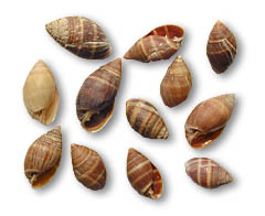
The following community data represent the abundances of three species of gastropods in five quadrats (ranging from high shore marsh - Quadrat 1, to low shore marsk - Quadrat 5) in a saltmarsh.

Download gastropod data set

Format of the gastropod

Salinator	Ophicardelus	Marinula
4	0	1
9	3	0
9	4	1
6	2	0
0	1	1

Salinator	Number of Salinator gastropods - variable
Ophicardelus	Number of Ophicardelus gastropods - variable
Marinula	Number of Marinula gastropods - variable
Q1-Q5	Quadrats - these are the objects

Open the gastropod data set.

Show code

> gastropod <- read.csv('../downloads/data/gastropod.csv')
> gastropod

  Salinator Ophicardelus Marinula
1         4            0        1
2         9            3        0
3         9            4        1
4         6            2        0
5         0            1        1

Using this very small data set, calculate both measures of association.

covariance

Show code

> cov(gastropod)

             Salinator Ophicardelus
Salinator        14.30         4.75
Ophicardelus      4.75         2.50
Marinula         -0.95        -0.25
             Marinula
Salinator       -0.95
Ophicardelus    -0.25
Marinula         0.30

correlation

Show code

> cor(gastropod)

             Salinator Ophicardelus
Salinator       1.0000       0.7944
Ophicardelus    0.7944       1.0000
Marinula       -0.4587      -0.2887
             Marinula
Salinator     -0.4587
Ophicardelus  -0.2887
Marinula       1.0000

In terms of species abundances at each site (rows), which species are most associated with one another?

Measures of association

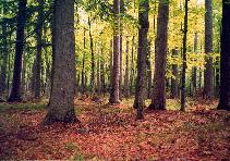
Peet & Loucks (1977) examined the abundances of 8 species of trees (Bur oak, Black oak, White oak, Red oak, American elm, Basswood, Ironwood, Sugar maple) at 10 forest sites in southern Wisconsin, USA. The data (given below) are the mean measurements of canopy cover for eight species of north American trees in 10 samples (quadrats). For this question we will explore the associations between the different species based on the degree to which their abundances in the quadrats match up (covary or correlate).

Download gastropod data set

Format of wisc.csv data file

QUAD.	BUROAK	BLACKOAK	WHITEOAK	REDOAK	ELM	BASSWOOD	IRONWOOD	MAPLE
1	9	8	5	3	2	0	0	0
2	8	9	4	4	2	0	0	0
3	3	8	9	0	4	0	0	0
4	5	7	9	6	5	0	0	0
5	6	0	7	9	6	2	0	0
6	0	0	7	8	5	7	6	5
7	5	0	4	7	5	6	7	4
8	0	0	6	6	0	6	4	8
9	0	0	0	4	2	7	6	8
10	0	0	2	3	5	6	5	9

QUADRAT	A number or name given to each quadrat
BUROAK, BLACKOAK,....	Number of individuals of each tree species found in each quadrat

Open the wisc data set.

Show code

> wisc <- read.csv('../downloads/data/wisc.csv')
> wisc

   QUADRAT BUROAK BLACKOAK WHITEOAK
1        1      9        8        5
2        2      8        9        4
3        3      3        8        9
4        4      5        7        9
5        5      6        0        7
6        6      0        0        7
7        7      5        0        4
8        8      0        0        6
9        9      0        0        0
10      10      0        0        2
   REDOAK ELM BASSWOOD IRONWOOD MAPLE
1       3   2        0        0     0
2       4   2        0        0     0
3       0   4        0        0     0
4       6   5        0        0     0
5       9   6        2        0     0
6       8   5        7        6     5
7       7   5        6        7     4
8       6   0        6        4     8
9       4   2        7        6     8
10      3   5        6        5     9

Calculate measures of association so as to:

reflect the actual levels of abundance of each species

Show code

> #exclude the first column as it is a list of quadrats and not abundances
> cov(wisc[,-1])

           BUROAK BLACKOAK WHITEOAK
BUROAK    12.2667    9.756    2.244
BLACKOAK   9.7556   17.289    4.600
WHITEOAK   2.2444    4.600    8.456
REDOAK    -0.2222   -6.444    1.000
ELM        0.2667   -1.578    1.689
BASSWOOD  -8.9333  -12.089   -5.022
IRONWOOD  -7.3111   -9.956   -4.933
MAPLE    -11.3778  -12.089   -7.022
          REDOAK     ELM BASSWOOD
BUROAK   -0.2222  0.2667  -8.9333
BLACKOAK -6.4444 -1.5778 -12.0889
WHITEOAK  1.0000  1.6889  -5.0222
REDOAK    7.3333  1.7778   3.1111
ELM       1.7778  3.8222  -0.1556
BASSWOOD  3.1111 -0.1556  10.4889
IRONWOOD  2.2222  0.1333   9.4222
MAPLE     0.5556 -1.8222  11.2667
         IRONWOOD    MAPLE
BUROAK    -7.3111 -11.3778
BLACKOAK  -9.9556 -12.0889
WHITEOAK  -4.9333  -7.0222
REDOAK     2.2222   0.5556
ELM        0.1333  -1.8222
BASSWOOD   9.4222  11.2667
IRONWOOD   9.2889   9.7556
MAPLE      9.7556  14.9333

reflect the relative abundances of each species (suppressing the influence of dominant species)

Show code

> cor(wisc[,-1])

           BUROAK BLACKOAK WHITEOAK
BUROAK    1.00000   0.6699   0.2204
BLACKOAK  0.66989   1.0000   0.3805
WHITEOAK  0.22038   0.3805   1.0000
REDOAK   -0.02343  -0.5723   0.1270
ELM       0.03894  -0.1941   0.2971
BASSWOOD -0.78756  -0.8977  -0.5333
IRONWOOD -0.68492  -0.7856  -0.5567
MAPLE    -0.84065  -0.7524  -0.6249
           REDOAK      ELM BASSWOOD
BUROAK   -0.02343  0.03894 -0.78756
BLACKOAK -0.57234 -0.19409 -0.89771
WHITEOAK  0.12699  0.29708 -0.53329
REDOAK    1.00000  0.33579  0.35473
ELM       0.33579  1.00000 -0.02457
BASSWOOD  0.35473 -0.02457  1.00000
IRONWOOD  0.26925  0.02238  0.95457
MAPLE     0.05309 -0.24119  0.90023
         IRONWOOD    MAPLE
BUROAK   -0.68492 -0.84065
BLACKOAK -0.78560 -0.75236
WHITEOAK -0.55666 -0.62492
REDOAK    0.26925  0.05309
ELM       0.02238 -0.24119
BASSWOOD  0.95457  0.90023
IRONWOOD  1.00000  0.82831
MAPLE     0.82831  1.00000

Note that the abundances of each species of tree in these data are fairly uniform. Each species has the similar minimum and maximum (and thus means and standard deviations). Indeed it is just elm and basswood that has slightly lower maximums and standard deviations). It is therefore just association measures involving either of those two species that are likely to differ in pattern between covariances and correlations.

If we were to standardize (scale) the raw abundances first (such that each species had a mean of 0 and a standard deviation of 1), the covariance measures would match the correlation measures of the raw data exactly. Recall that such a standardization effectively evens up the relative abundances of each species. Try it to prove it to yourself.

Show code

> library(vegan)
> cov(decostand(wisc[,-1], method = "standardize"))

           BUROAK BLACKOAK WHITEOAK
BUROAK    1.00000   0.6699   0.2204
BLACKOAK  0.66989   1.0000   0.3805
WHITEOAK  0.22038   0.3805   1.0000
REDOAK   -0.02343  -0.5723   0.1270
ELM       0.03894  -0.1941   0.2971
BASSWOOD -0.78756  -0.8977  -0.5333
IRONWOOD -0.68492  -0.7856  -0.5567
MAPLE    -0.84065  -0.7524  -0.6249
           REDOAK      ELM BASSWOOD
BUROAK   -0.02343  0.03894 -0.78756
BLACKOAK -0.57234 -0.19409 -0.89771
WHITEOAK  0.12699  0.29708 -0.53329
REDOAK    1.00000  0.33579  0.35473
ELM       0.33579  1.00000 -0.02457
BASSWOOD  0.35473 -0.02457  1.00000
IRONWOOD  0.26925  0.02238  0.95457
MAPLE     0.05309 -0.24119  0.90023
         IRONWOOD    MAPLE
BUROAK   -0.68492 -0.84065
BLACKOAK -0.78560 -0.75236
WHITEOAK -0.55666 -0.62492
REDOAK    0.26925  0.05309
ELM       0.02238 -0.24119
BASSWOOD  0.95457  0.90023
IRONWOOD  1.00000  0.82831
MAPLE     0.82831  1.00000

Distance measures

We return again to the abundances of three species of gastropods in five quadrats (ranging from high shore marsh - Quadrat 1, to low shore marsk - Quadrat 5) in a saltmarsh.

Download gastropod data set

Format of the gastropod

Salinator	Ophicardelus	Marinula
4	0	1
9	3	0
9	4	1
6	2	0
0	1	1

Salinator	Number of Salinator gastropods - variable
Ophicardelus	Number of Ophicardelus gastropods - variable
Marinula	Number of Marinula gastropods - variable
Q1-Q5	Quadrats - these are the objects

Open the gastropod data set.

Show code

> gastropod <- read.csv('../downloads/data/gastropod.csv')
> gastropod

  Salinator Ophicardelus Marinula
1         4            0        1
2         9            3        0
3         9            4        1
4         6            2        0
5         0            1        1

We will use these data to explore a range of distance matrices

Euclidean distance

Show code

> library(vegan)
> vegdist(gastropod, "euc")

      1     2     3     4
2 5.916                  
3 6.403 1.414            
4 3.000 3.162 3.742      
5 4.123 9.274 9.487 6.164

Bray-Curtis dissimilarity

Show code

> library(vegan)
> vegdist(gastropod, "bray")

        1       2       3       4
2 0.52941                        
3 0.47368 0.07692                
4 0.38462 0.20000 0.27273        
5 0.71429 0.85714 0.75000 0.80000

Measures of association

Finally, we return to Peet & Loucks (1977) Wisconsin tree data. For this question we will explore the similarities of quadrats (objects) based on how well the abundances of each species match up.

Download gastropod data set

Format of wisc.csv data file

QUAD.	BUROAK	BLACKOAK	WHITEOAK	REDOAK	ELM	BASSWOOD	IRONWOOD	MAPLE
1	9	8	5	3	2	0	0	0
2	8	9	4	4	2	0	0	0
3	3	8	9	0	4	0	0	0
4	5	7	9	6	5	0	0	0
5	6	0	7	9	6	2	0	0
6	0	0	7	8	5	7	6	5
7	5	0	4	7	5	6	7	4
8	0	0	6	6	0	6	4	8
9	0	0	0	4	2	7	6	8
10	0	0	2	3	5	6	5	9

QUADRAT	A number or name given to each quadrat
BUROAK, BLACKOAK,....	Number of individuals of each tree species found in each quadrat

Open the wisc data set.

Show code

> wisc <- read.csv('../downloads/data/wisc.csv')
> wisc

   QUADRAT BUROAK BLACKOAK WHITEOAK
1        1      9        8        5
2        2      8        9        4
3        3      3        8        9
4        4      5        7        9
5        5      6        0        7
6        6      0        0        7
7        7      5        0        4
8        8      0        0        6
9        9      0        0        0
10      10      0        0        2
   REDOAK ELM BASSWOOD IRONWOOD MAPLE
1       3   2        0        0     0
2       4   2        0        0     0
3       0   4        0        0     0
4       6   5        0        0     0
5       9   6        2        0     0
6       8   5        7        6     5
7       7   5        6        7     4
8       6   0        6        4     8
9       4   2        7        6     8
10      3   5        6        5     9

Calculate distance/dissimilarity indices such that they:

reflect the actual straight-line distances between each pair of points in multi-variate space

Show code

> #exclude the first column as it is a list of quadrats and not abundances
> library(vegan)
> vegdist(wisc[,-1],"euc")

        1      2      3      4      5
2   2.000                            
3   8.062  8.426                     
4   7.141  7.141  6.481              
5  11.533 11.790 12.884  8.246       
6  17.117 17.000 15.875 13.856 11.136
7  14.387 14.457 15.620 13.266  9.798
8  16.583 16.523 15.811 14.967 13.342
9  17.889 17.607 17.972 17.804 15.843
10 17.464 17.349 16.553 16.553 14.832
        6      7      8      9
2                             
3                             
4                             
5                             
6                             
7   6.164                     
8   6.633  8.944              
9   9.110  8.775  7.000       
10  8.246  8.602  7.211  4.123

reflect the similarity of quadrats only on the basis of what they do share and not what they do not share (ignore shared absences)

Show code

> #exclude the first column as it is a list of quadrats and not abundances
> library(vegan)
> vegdist(wisc[,-1],"bray")

         1       2       3       4
2  0.07407                        
3  0.29412 0.33333                
4  0.25424 0.25424 0.17857        
5  0.43860 0.43860 0.48148 0.25806
6  0.69231 0.69231 0.64516 0.48571
7  0.56923 0.53846 0.64516 0.42857
8  0.71930 0.71930 0.77778 0.61290
9  0.81481 0.77778 0.92157 0.79661
10 0.75439 0.75439 0.77778 0.67742
         5       6       7       8
2                                 
3                                 
4                                 
5                                 
6  0.35294                        
7  0.32353 0.15789                
8  0.53333 0.20588 0.29412        
9  0.71930 0.26154 0.32308 0.22807
10 0.60000 0.23529 0.26471 0.23333
         9
2         
3         
4         
5         
6         
7         
8         
9         
10 0.15789

Note, in the case of Bray-Curtis dissimilarity, it is common practice to first perform some sort of standardization of the data so as to even up the influence of all species and sites irrespective of whether they are abundant or rate (such as a Wisconsin double standardization).