Tutorial 15.1 - Multidimensional Scaling (MDS)

12 Mar 2015

View R code for preliminaries.

> library(vegan)
> library(ggplot2)
> library(grid)
> #define my common ggplot options
> murray_opts <- opts(panel.grid.major=theme_blank(),
+                            panel.grid.minor=theme_blank(),
+                            panel.border = theme_blank(),
+                            panel.background = theme_blank(),
+                            axis.title.y=theme_text(size=15, vjust=0,angle=90),
+                            axis.text.y=theme_text(size=12),
+                            axis.title.x=theme_text(size=15, vjust=-1),
+                            axis.text.x=theme_text(size=12),
+                            axis.line = theme_segment(),
+                            plot.margin=unit(c(0.5,0.5,1,2),"lines")
+ )

Error: Use 'theme' instead. (Defunct;
last used in version 0.9.1)

> coenocline <- function(x,A0,m,r,a,g, int=T, noise=T) {
+ #x is the environmental range
+ #A0 is the maximum abundance of the species at the optimum environmental conditions
+ #m is the value of the environmental gradient that represents the optimum conditions for the species
+ #r the species range over the environmental gradient (niche width)
+ #a and g are shape parameters representing the skewness and kurtosis
+ # when a=g, the distribution is symmetrical
+ # when a>g - negative skew (large left tail)
+ # when a<g - positive skew (large right tail)
+ #int - indicates whether the responses should be rounded to integers (=T)
+ #noise - indicates whether or not random noise should be added (reflecting random sampling)  
+ #NOTE.  negative numbers converted to 0
+          b <- a/(a+g)
+          d <- (b^a)*(1-b)^g
+          cc <- (A0/d)*((((x-m)/r)+b)^a)*((1-(((x-m)/r)+b))^g)
+          if (noise) {n <- A0/10; n[n<0]<-0; cc<-cc+rnorm(length(cc),0,n)}
+          cc[cc<0] <- 0
+          cc[is.na(cc)]<-0
+          if (int) cc<-round(cc,0)
+          cc
+ }
> #plot(coenocline(0:100,40,40,20,1,1, int=T, noise=T), ylim=c(0,100))

To assist with demonstrating Multidimensional Scaling (MDS), we will return to the fabricated species abundance data introduced in Tutorial 13.2. This data set comprises the abundances of 10 species within 10 sites located along a transect that extends in a northerly direction over a mountain range.

Details of data generation

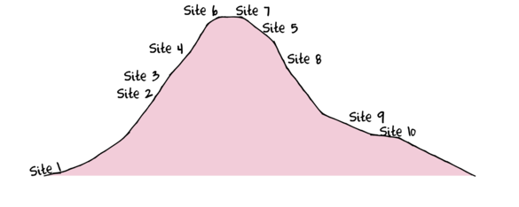
> set.seed(1)
> x <- seq(0,50,l=10)
> n <- 10
> sp1<-coenocline(x=x,A0=5,m=0,r=2,a=1,g=1,int=T, noise=T)
> sp2<-coenocline(x=x,A0=70,m=7,r=30,a=1,g=1,int=T, noise=T)
> sp3<-coenocline(x=x,A0=50,m=15,r=30,a=1,g=1,int=T, noise=T)
> sp4<-coenocline(x=x,A0=7,m=25,r=20,a=0.4,g=0.1,int=T, noise=T)
> sp5<-coenocline(x=x,A0=40,m=30,r=30,a=0.6,g=0.5,int=T, noise=T)
> sp6<-coenocline(x=x,A0=15,m=35,r=15,a=0.2,g=0.3,int=T, noise=T)
> sp7<-coenocline(x=x,A0=20,m=45,r=25,a=0.5,g=0.9,int=T, noise=T)
> sp8<-coenocline(x=x,A0=5,m=45,r=5,a=1,g=1,int=T, noise=T)
> sp9<-coenocline(x=x,A0=20,m=45,r=15,a=1,g=1,int=T, noise=T)
> sp10<-coenocline(x=x,A0=30,m=50,r=5,a=1,g=1,int=T, noise=T)
> X <- cbind(sp1, sp10,sp9,sp2,sp3,sp8,sp4,sp5,sp7,sp6)
> #X<-X[c(1,10,9,2,3,8,4,5,7,6),] 
> colnames(X) <- paste("Sp",1:10,sep="")
> rownames(X) <- paste("Site", c(1,10,9,2,3,8,4,5,7,6), sep="")
> X <- X[c(1,4,5,7,8,10,9,6,3,2),]
> data <- data.frame(Sites=factor(rownames(X),levels=rownames(X)), X)

Sites	Sp1	Sp2	Sp3	Sp4	Sp5	Sp6	Sp7	Sp8	Sp9	Sp10
Site1	5	0	0	65	5	0	0	0	0	0
Site2	0	0	0	25	39	0	6	23	0	0
Site3	0	0	0	6	42	0	6	31	0	0
Site4	0	0	0	0	0	0	0	40	0	14
Site5	0	0	6	0	0	0	0	34	18	12
Site6	0	29	12	0	0	0	0	0	22	0
Site7	0	0	21	0	0	5	0	0	20	0
Site8	0	0	0	0	13	0	6	37	0	0
Site9	0	0	0	60	47	0	4	0	0	0
Site10	0	0	0	72	34	0	0	0	0	0

Q-mode analyses

In contrast to R-mode analyses (such as principle components analysis), Q-mode analyses explore the patterns between objects (sites) on the basis of pairwise object likenesses (c.f. associations between variables). Whereas the starting point of R-mode analyses is typically either a covariance or correlation matrix and matrix algebra is used to arrange objects (sites) so as to preserve either their euclidean distances (PCA/RDA) or $\chi^2$ distances (CA/CCA), Q-mode analyses (such as MDS) provide euclidean or arbitrary (where only the order is preserved) ordination distances from any distance or similarity matrix.

This unrestricted choice of starting distance matrix provides enormous flexibility to be able to handle a wide range of data and issues. The distance matrix is selected to best reflect the nature of the data and thus acts as a sort of filter or conduit through which data are converted into a form suitable for analysis.

A consequence of basing analyses on distance matrices is that the resulting axes scores (coordinates) or patterns are not independent of one another. That is, the new values along a particular axes are all non-independent. Consequently, the new variables (dimensions) cannot be used in traditional linear modelling (c.f. PCA).

Multidimensional Scaling

The main function of multidimensional Scaling (MDS) is to re-project the objects (sites) in reduced dimension ordination space. As stated above, the axes scores cannot be used in subsequent analyses due to a lack of independence.

The real advantage of MDS over other ordination techniques is that it will generally represent the ordering relationships amongst objects within a given set of dimensions better than eigen-based ordinations. Whilst the eigen-based analyses rotates all of the original axes such that each axis maximizes the variance preserved by that axes, MDS constructs a configuration of objects specifically for only a nominated number of new axes. Therefore, when a 2 dimensional ordination is desired, the configuration from an MDS is optimized for just two dimensions whereas the eigen-based object configurations are independent of how many dimensions you intend to plot.

Principle components analysis (PCA) can be performed by either spectral (eigen) decomposition of an association matrix or single value decomposition of the original data matrix. Either way, it yields a rigid rotation of axes in that the positions of points relative to one another (euclidean distances) are maintained during rotation. The rotated axes are referred to as principle components.

Obviously, the higher the degree of associations between the variables (species), the more strongly focused and oriented the data cloud is and therefore the more 'successful' the PCA in terms of being able to represent many variables by only a few new variables.

The resulting principle components (axes) and scores (new variable values) are independent of one another and therefore the 'reduced data' can be used in subsequent statistical analyses. For example, principle component 1 (as one measure of the community) could be regressed against an environmental variable (such as altitude or rainfall) in a regular linear modelling procedure. Similarly, multiple correlated predictor variables (that otherwise violate multi-collinearity) could be reduced to one or two orthogonal predictors to use in linear modelling. Principle components analysis is therefore often an intermediate step to used as either responses or predictors in linear modeling.

MDS is mathematically and conceptually relatively simple, yet computationally very intense. Rather than have elegant mathematical solutions, MDS works on bruit grunt.

We will now attempt to conceptualize the process of multidimensional scaling

Generate a distance (dissimiliarity) matrix from the multivariate data. For the purpose of this demonstration (and since the data are species abundances), we will use a Bray-Curtis dissimilarity matrix.

> data.dist <- vegdist(data[,-1], "bray")
> data.dist

        Site1  Site2  Site3  Site4
Site2  0.6429                     
Site3  0.8625 0.1685              
Site4  1.0000 0.6871 0.5540       
Site5  1.0000 0.7178 0.6000 0.2581
Site6  1.0000 1.0000 1.0000 1.0000
Site7  1.0000 1.0000 1.0000 1.0000
Site8  0.9237 0.4362 0.2908 0.3273
Site9  0.3011 0.3333 0.4694 1.0000
Site10 0.2265 0.4070 0.5812 1.0000
        Site5  Site6  Site7  Site8
Site2                             
Site3                             
Site4                             
Site5                             
Site6  0.6391                     
Site7  0.5862 0.4128              
Site8  0.4603 1.0000 1.0000       
Site9  1.0000 1.0000 1.0000 0.7964
Site10 1.0000 1.0000 1.0000 0.8395
        Site9
Site2        
Site3        
Site4        
Site5        
Site6        
Site7        
Site8        
Site9        
Site10 0.1336

Note that this is a triangular matrix - the diagonals (which would all be 0) and the upper right cells (which are a mirror of the lower left cells) are omitted. For the remainder of this demonstration, we will represent this dissimilarity matrix as:

Decide on how many dimensions are required of the final ordination plot - how many dimensions do you want to visualize the objects (sites) in? Choice of the number of dimensions is typically a compromise between ease of visualization (fewer dimensions) and sufficiently capturing the patterns in the original data (more dimensions). Two or three dimensions is usually a decent compromise that is nonetheless based more on ease of visualization.
Having nominated the number of ordination dimensions (in this case 2), we then randomly arrange our sites in two dimensions.
We now measure how well this configuration (arrangement of sites on the ordination) match the original distance (dissimilarity) matrix. That is, we measure how well the two new axes represent the patterns that existed across all the original variables (species). We do this by creating a matrix of distances between all of the points on the ordination. These are called ordination distances and are simply the euclidean (straight-line) distances between each point and each other point.
The degree of agreement between the data distance and ordination distance matrices is usually explored by fitting a regression model. The relationship can also be visualized in a Shepard diagram. The Shepard plots ordination distances (y-axis) against data distances (x-axis).

Obviously since the sites have just been placed in ordination space at random, there will initially be a very low degree of correspondence between the original data distance matrix and the new ordination distance matrix.

The goodness of fit of the regression between data and ordination distances is measured by a property called stress. There are basically two forms of stress:
- Kruskal's stress $$stress = \sqrt{\frac{\sum{(D_{ord.i}-D_{data.i})^2}}{\sum{D_{ord.i^2}}}}$$
- Modified Kruskal's stress $$stress = \sqrt{\frac{\sum{(D_{ord.i}-D_{data.i})^2}}{\sum{D_{ord.i^2}-\bar{D_{data.i}}}}}$$ The modified Kruskal's stress is equivalent to $\sqrt(1-R^2)$
Either way, stress values less than 0.2 are considered good. The smaller the stress value, the better the match between data and ordination distances and thus the better the new two-dimensional configuration represents the patterns based on all the original variables.
The configuration of points on the ordination is then "improved" by shifting the position of the points slightly. Points are shifted via a process called gradient descent which ensures that points are shifted in the direction that will cause the stress value to be reduced by the greatest amount (the steepest descent).
The points are repeatedly (iteratively) adjusted. Each time the correlation between data and ordination distances will improve.
At first, successive iterations will yield marked improvements in the correlation between data and ordination distances (and thus large improvements in stress). However, eventually the improvements will be very minor.
The iterative process could in theory go on indefinitely. However as the rate of improvement diminishes with each additional iteration, there comes a point were the improvements become imperceptible. There is also the possibility that there was no real patter in the original data and therefore no amount of exhaustive reconfiguration is going to yield patterns in reduced ordination space.
There are typically three stopping rules in place that indicate when the iterative reconfiguration process should cease.
1. convergence tolerance - iterations stop when the stress value falls below a threshold (such as stress=0.001)
2. the stress ratio (ratio of the stress values for the current and previous iterations) - iterations stop once the improvement in stress falls below a threshold (such as 1.1)
3. maximum iterations - iterations stop once a set number of iterations have occurred (such as 200).

Ideally, we are seeking a stress value of less than 0.2. This roughly corresponds to the ordination distances (and thus the new axes from which they are derived) explaining 80% of the variability in the data dissimilarity matrix (which is based on all the original variables). Hence if we have a stress value of 0.2 or less, then we can be increasingly more confident that we have been able to encapsulate the major patterns.

The final configuration displays an arrangement of objects (sites) in two (or three) dimensions in which the rank proximity of points to one another is proportional to how alike the sites are in their community structure. Note however, the axes themselves have no real meaning. Unlike principle components analysis or correspondence analysis in which the axes reflect major underlying gradients, the orientation of points with respect to the MDS axes are somewhat arbitrary. Instead the axes operate together just to create the ordination space and the configuration can be oriented at any angle to the axes. That said, it is possible to lock the orientation of the configuration so as to give the individual axes more meaning.

Starting configuration

The starting configuration can (as demonstrated above) be any random arrangement of points in the nominated dimensions. Alternatively, the starting configuration can be approximated by first running an eigen-analysis based ordination (similar to a PCA, yet using a distance matrix rather than an association matrix). Not only does this usually reduce the risks of running into local minimum issues (see below), it can also drastically reduce the number of iteration required for the iterations to converge.

The final configuration can be dependent on the starting configuration (i.e. the initial arrangement of sites). The gradient descent algorithms can get stuck in what are called local minimums (or optimums). This occurs when the math limits the possible position adjustments that can be made and the small alterations possible within the scope of the algorithms are insufficient to bring about substantial improvements. In these cases, more drastic adjustments would be required in order to free up the algorithm to find true minimums (better configurations).

Therefore, it is usually good practice to repeat the entire process multiple times, each time with a different random starting configuration.

Procrustes rotation

The final stress value of a final configuration is a good indicator of how good the configuration is. We could therefore, run the analysis multiple times (each time with a different starting configuration) and ultimately select the final configuration that has the lowest stress value. However, this might lead to many extraneous runs. It may be that the data and patterns are sufficiently strong and stable that any two runs would result in essentially the same configuration (irrespective of initial configuration). What is required is a means to evaluate when the final configurations of two runs are essentially the same (when they have converged on the same solution).

Unlike eigen-based analysis (such as PCA) in which the first axis represents the orientation of data in the plane of greatest variance and each subsequent axis represents the greatest direction of remaining variance, in MDS, the orientation and scaling of points with respect to the axes are of no meaning. The two (or three) axes simply define the ordination space in which the point can be plotted. Consequently it can often be difficult to judge how similar two configurations are - they might be identical, yet one is upside down and twice as wide (for example).

Consider the following two final configurations resulting from the same dissimilarity matrix and with the same number of iterations and differing only in their starting configurations.

If we rotated the configuration on the right clockwise approximately 45 degrees, these points would superimpose almost exactly onto the configuration on the left. This can be seen in the figure below (left). The previous best configuration is depicted in solid black and the latest configuration is depicted in light red and solid red when scaled and rotated and superimposed. Blue arrows indicated the amount that each point is transformed. The figure on the right indicates the differences (residuals) between the two configurations (once projection on the same scale and rotation) as solid red lines.

This process of comparing the two final configurations by scaling and rotating one configuration (the latest configuration) and superimposing it upon another (the previous best configuration - the standard) is called Procrustes rotation. The amount of scaling and rotation is selected so as to minimize the sum of the squared distances (residuals - the red lines in the figure above) between the two sets of points (analogous to the way a regression line is fitted such that the squared deviations from the line are minimized). This minimum sum of squares is called the root mean square error (rmse). The smaller the rmse, the more similar the two configurations are.

Two final configurations are considered to have converged (arrived at essentially the same solution) when the rmse is less than 0.01, and no single residual value exceeds 0.005. Procrustes analysis thereby provides a mechanism for determining when to stop repeatedly re-running the analysis - stop when there is convergence as measured by procrustes rmse.

MDS options

There is not just one single multidimensional scaling process. Rather, there are many different process and options, each of which alters some aspect of the behavior of the MDS. Here are some of the more major choices:

metric versus non-metric. This is a fundamental distinction between those MDS's that base stress (and therefore the stopping criterion) on metric regression (essentially linear regression) and those that base stress on monotonic (essentially non-linear) regression. For most ecological data, the relationship between data dissimilarity and ordination distance will be non-linear. Consequently, non-metric multidimensional scaling (NMDS) is preferred by ecologists.
Within NMDS, there is a further distinction between whether the regression should be:
- monotonic regression
- or an equivalent of a locally weighted regression separate for each point
how to generate the initial or starting configuration. The MDS can either start with a completely random configuration or the configuration can be leveraged from other means.
whether or not to automatically employ multiple random starts.
whether an how to scale the axes scores. This can make the ordinations easier to interpret.

In addition to being able to supply any dissimilarity matrix as input, there are a wide variety of other parameters that

In R, MDS is implemented several functions (although I will only mention two per method).

metric MDS is performed by either cmdscale() or metaMDS() (vegan)
non-metric MDS is performed by either isoMDS() or metaMDS() (vegan).

Of the above, the metaMDS function is the most comprehensive, offering an MDS interface to just about all MDS routines. Consequently, this is the one will be focus on.

`metaMDS()`

The metaMDS() function does not itself perform multidimensional scaling. Rather it is a short-cut wrapper that brings together each of the important steps in performing multidimensional scaling.

If the metaMDS() function is provided raw community data, it will:
- transform and/or standardize the data. Depending on the magnitude of the abundances, data will be square-root transformed before being subject to a Wisconsin double standardization (column maximum followed by row total). This behavior can be suppressed via the autotransform=FALSE argument to allow full control over transformations and standardizations.
- generate a dissimilarity matrix. The vegdist() function is called to generate a dissimilarity matrix. By default this is a Bray-Curtis dissimilarity, however, any of the distances supported by vegdist() can be nominated.
The above steps are skipped if the metaMDS() function is provided with a dissimilarity matrix (matrix of class dist) instead of a raw data matrix.
The MDS engine is called. By default this is the monoMDS() function also in the vegan package, although it is also possible to specify isoMDS() as an alternative.
- The initial starting configuration (if not provided) is generated via metric scaling (principle coordinates analysis - PCoA). PCoA is essentially a PCA performed on a distance matrix.
  Thereafter, the monoMDS() engine function is called repeatedly (up to trymax=20 times), each time with a new completely random starting configuration. Each time monoMDS is called, the engine iteratively adjusts the positions of points on the ordination space and evaluates the stress with respect to the stopping criterion.
- The final stress value from each new run of the monoMDS() function is compared to the final stress value from the previous 'best' run and if the new stress value is better (lower), then the final configurations of the previous best and the latest runs are compared via Procrustes analysis to establish whether they might have converged (essentially arrived at the same configuration). If they have converged, the configuration with the lower stress value is considered the 'best' configuration.
Following the arrival of the final configuration, the results are scaled to allow:
- center the origin (0,0) to the average of the axes scores
- either principle components-like rotation of the configuration so as to mimic the way the first axis of a PCA represents the orientation of the greatest variance or rotating the configuration such that the first axis (dimension) is parallel to an environmental variable.
Finally, variable (species) axes scores are generated as the weighted averages.

Most of the default settings used in metaMDS() were designed with community (species abundance) data in mind.

Our example data set is species abundance data, and therefore the defaults (Wisconsin double standardization, Bray-Curtis dissimilarity, non-metric multidimensional scaling with multiple random starts followed by centering and principle components-like rotation of the configuration, would seem appropriate.

> library(vegan)
> data.nmds <- metaMDS(data[,-1])

Square root transformation
Wisconsin double standardization
Run 0 stress 0.03499 
Run 1 stress 9.419e-05 
... New best solution
... procrustes: rmse 0.115  max resid 0.2088 
Run 2 stress 0.0005712 
... procrustes: rmse 0.1885  max resid 0.2961 
Run 3 stress 0.0004598 
... procrustes: rmse 0.1281  max resid 0.2567 
Run 4 stress 0.1072 
Run 5 stress 0.08642 
Run 6 stress 0.000249 
... procrustes: rmse 0.1767  max resid 0.2933 
Run 7 stress 9.78e-05 
... procrustes: rmse 0.1051  max resid 0.2432 
Run 8 stress 9.692e-05 
... procrustes: rmse 0.1516  max resid 0.3103 
Run 9 stress 9.796e-05 
... procrustes: rmse 0.1283  max resid 0.2929 
Run 10 stress 9.757e-05 
... procrustes: rmse 0.06026  max resid 0.0896 
Run 11 stress 9.905e-05 
... procrustes: rmse 0.1624  max resid 0.3806 
Run 12 stress 0.07878 
Run 13 stress 9.678e-05 
... procrustes: rmse 0.008004  max resid 0.01477 
Run 14 stress 0.001213 
Run 15 stress 0.002591 
Run 16 stress 9.385e-05 
... New best solution
... procrustes: rmse 0.1073  max resid 0.2635 
Run 17 stress 9.784e-05 
... procrustes: rmse 0.1069  max resid 0.2275 
Run 18 stress 0.00139 
Run 19 stress 9.781e-05 
... procrustes: rmse 0.02273  max resid 0.04333 
Run 20 stress 9.553e-05 
... procrustes: rmse 0.1389  max resid 0.2901

The returned message indicates:

the original data was subject to square-root transformation followed by a Wisconsin double standardization.
a total of 20 random starts (default) were attempted. For each run, the final stress is given and when a stress value similar to the lowest is achieved, a procrustes analysis determines the rmse and maximum residual value (to determine whether convergence has occurred).
The rmse value did not fall bellow 0.01 and therefore convergence was not considered to have occurred prior to the completion of the set number of random starts.

We could repeat the entire process and nominate a larger number of random starts in order to strive for convergence. However, in this case, the stress value of the first run is very low (as is the stress of any one of the candidate configurations), indicating that they are good approximations of the original patterns. Hence we might be satisfied with just accepting the 'best' so far. This is the configuration stored in the metaMDS object.

Additional information is gained by printing the object.

> data.nmds

Call:
metaMDS(comm = data[, -1]) 

global Multidimensional Scaling using monoMDS

Data:     wisconsin(sqrt(data[, -1])) 
Distance: bray 

Dimensions: 2 
Stress:     9.385e-05 
Stress type 1, weak ties
No convergent solutions - best solution after 20 tries
Scaling: centring, PC rotation, halfchange scaling 
Species: expanded scores based on 'wisconsin(sqrt(data[, -1]))'

we are reminded that the configuration is for two dimensions
the final stress of the 'best' configuration is indicated
we are reminded of any scaling and rotations that might have been applied to the axes scores. In this case, the scores were centered and rotated to emulate the way PCA orients axes according to planes of greatest variance.
we are informed that variable (species) scores have also been calculated as the means of each of the site scores weighted by the square-root species abundances.

Lets examine the Shepard (stress) plot to get a feel for how well the configuration in two dimensions matches the original data patterns.

> stressplot(data.nmds)

The fit between the community distances (data dissimilarity) and ordination distances is indicated by the monotonic step line (red).
Two stress values are provided:
- Non-metric fit - this is the modified Kruskal's stress value and is $\sqrt{1-R^2}$
- Linear fit - this is the $R^2$ value of the correlation between the ordination values and the ordination values predicted from the (monotonic) regression line.
For non-metric MDS the two stress values are the same.

> ordiplot(data.nmds, type="text")

Interpreting axes in terms of environmental variables

Establishing relationships between MDS axes and environmental variables is not as straight forward as it is in PCA. Firstly, the orientation of sites in MDS reduced ordination space is largely arbitrary. Thus, in order to relate them to changes in environmental factors, the only sensible way to orient the axes is in accordance to planes of greatest variability (similar to PCA). So the axes scores must first be rotated accordingly.

Secondly, as mentioned previously, as the axes scores are based on distance measures (which are themselves derived from the patterns between objects (sites), they scores are not independent of one another. Consequently, they violate one of the main assumptions of inferential statistics.

Nevertheless, environmental variables can be overlayed onto the ordination plot in a similar way as the species scores are overlayed. Lets first retrieve the environmental variables collected from the 10 sites.

Details of data generation

> set.seed(1)
> Site <- gl(10,1,10,lab=paste('Site',1:10, sep=""))
> Y <- matrix(c(
+ 6.1,4.2,101325,2,
+ 6.7,9.2,101352,510,
+ 6.8,8.6,101356,546,
+ 7.0,7.4,101372,758,
+ 7.2,5.8,101384,813,
+ 7.5,8.4,101395,856,
+ 7.5,0.5,101396,854,
+ 7.0,11.8,101370,734,
+ 8.4,8.2,101347,360,
+ 6.2,1.5,101345,356
+   ),10,4, byrow=TRUE)
> colnames(Y) <- c('pH','Slope', 'Pressure', 'Altitude')
> Substrate <- factor(c('Quartz','Shale','Shale','Shale','Shale','Quartz','Quartz','Shale','Quartz','Quartz'))
> enviro <- data.frame(Site,Y,Substrate)

We can now explore these environmental variables by over laying them on the ordination space.

> ordiplot(data.nmds, type="text")
> data.envfit <- envfit(data.nmds,enviro[,-1])
> plot(data.envfit)

Altitude, pressure and pH all seem to align predominantly with axis 1 (particularly pressure)
Temperature and slope align almost entirely with axis 2.
Arrow length is proportional to the degree of correlation between the environmental variable and the ordination

Whilst traditional inference tests are invalid (due to a violation of independence), permutation based tests are possible. Permutation tests compare a test statistic calculated from the observed data to a large number of such values generated by repeatedly shuffling the actual data. The basic premise is to see how often a test statistic of the magnitude observed from the actual data could be achieved just by pure chance (hence the reshuffling). The frequency of occasions that the observed test statistic is greater than the randomized test statistics is the p-value.

The envfit() function performs one such permutation test and is based on comparing the observed $R^2$ to a large number of $R^2$ values from repeatedly shuffling the rows of the environmental data.

> data.envfit

***VECTORS

          NMDS1  NMDS2   r2 Pr(>r)    
pH        0.976 -0.217 0.20  0.471    
Slope    -0.331 -0.944 0.39  0.176    
Pressure  0.975 -0.224 0.90  0.001 ***
Altitude  0.833 -0.553 0.86  0.001 ***
---
Signif. codes:  
  0 '***' 0.001 '**' 0.01 '*' 0.05
  '.' 0.1 ' ' 1
P values based on 999 permutations.

***FACTORS:

Centroids:
                NMDS1 NMDS2
SubstrateQuartz  0.06  0.59
SubstrateShale  -0.06 -0.59

Goodness of fit:
            r2 Pr(>r)
Substrate 0.25   0.11
P values based on 999 permutations.

For each of the environmental variables the table displays:
- the cosine of the angle to each axis
- the $R^2$ of the relationship between the environmental variable and the ordination
- permutation-based p-value
The chances of obtaining the relationships between ordination and Temperature, Pressure and Altitude by chance are all very low ($<0.05$), hence we conclude that Temperature, Pressure and Altitude are all correlated to community structure.

There are numerous alternative ways of performing permutation test (based on other test statistics and randomization schedules), some of which will be explored in Tutorial 15.2.

Worked Examples

Basic statistics references

Legendre and Legendre
Quinn & Keough (2002) - Chpt 17

Non-metric Multidimensional Scaling (NMDS)

The following example is designed to help you appreciate the link between distance measures and ordination space (MDS). The data set consists of distances (km) between major Australia cities (as the crow flies), and is in the form of a triangular matrix.

Download austcities data set

Format of austcites.csv data file

	Canberra	Sydney	Melbourne	..
Canberra	0	NA	NA	..
Sydney	246	0	NA	..
Melbourne	467	713	0	..
Adelaide	958	1160	653	..
Perth	3090	3290	2720	..
..	..	..	..	..

Open the veg data set.

Show code

> austcities <- read.csv('../downloads/data/austcities.csv')
> austcities

           Canberra Sydney Melbourne
Canberra          0     NA        NA
Sydney          246      0        NA
Melbourne       467    713         0
Adelaide        958   1160       653
Perth          3090   3290      2720
Broome         3280   3380      3120
Alice          1950   2030      1890
Darwin         3130   3150      3150
Cairns         2060   1960      2320
Townsville     1790   1680      2070
Brisbane        941    731      1370
Hobart          860   1060       597
           Adelaide Perth Broome Alice
Canberra         NA    NA     NA    NA
Sydney           NA    NA     NA    NA
Melbourne        NA    NA     NA    NA
Adelaide          0    NA     NA    NA
Perth          2130     0     NA    NA
Broome         2490  1680      0    NA
Alice          1330  1990   1370     0
Darwin         2620  2650   1110  1290
Cairns         2120  3440   2500  1450
Townsville     1920  3390   2590  1420
Brisbane       1600  3610   3320  1960
Hobart         1160  3010   3640  2460
           Darwin Cairns Townsville
Canberra       NA     NA         NA
Sydney         NA     NA         NA
Melbourne      NA     NA         NA
Adelaide       NA     NA         NA
Perth          NA     NA         NA
Broome         NA     NA         NA
Alice          NA     NA         NA
Darwin          0     NA         NA
Cairns       1680      0         NA
Townsville   1860    281          0
Brisbane     2850   1390       1110
Hobart       3730   2890       2630
           Brisbane Hobart
Canberra         NA     NA
Sydney           NA     NA
Melbourne        NA     NA
Adelaide         NA     NA
Perth            NA     NA
Broome           NA     NA
Alice            NA     NA
Darwin           NA     NA
Cairns           NA     NA
Townsville       NA     NA
Brisbane          0     NA
Hobart         1790      0

Note the format of the file, it is a triangular distance matrix.

While the file is a distance matrix, at this stage R is unaware of it, we must manually make it aware (a round about way of saying that we must type a command to force R to treat the data set as a distance matrix. Convert the data frame into a distance matrix (HINT).

Show code

> austcities <- as.dist(austcities)
> austcities

           Canberra Sydney Melbourne
Sydney          246                 
Melbourne       467    713          
Adelaide        958   1160       653
Perth          3090   3290      2720
Broome         3280   3380      3120
Alice          1950   2030      1890
Darwin         3130   3150      3150
Cairns         2060   1960      2320
Townsville     1790   1680      2070
Brisbane        941    731      1370
Hobart          860   1060       597
           Adelaide Perth Broome Alice
Sydney                                
Melbourne                             
Adelaide                              
Perth          2130                   
Broome         2490  1680             
Alice          1330  1990   1370      
Darwin         2620  2650   1110  1290
Cairns         2120  3440   2500  1450
Townsville     1920  3390   2590  1420
Brisbane       1600  3610   3320  1960
Hobart         1160  3010   3640  2460
           Darwin Cairns Townsville
Sydney                             
Melbourne                          
Adelaide                           
Perth                              
Broome                             
Alice                              
Darwin                             
Cairns       1680                  
Townsville   1860    281           
Brisbane     2850   1390       1110
Hobart       3730   2890       2630
           Brisbane
Sydney             
Melbourne          
Adelaide           
Perth              
Broome             
Alice              
Darwin             
Cairns             
Townsville         
Brisbane           
Hobart         1790

We are now ready to perform the MDS for the purpose of examining the ordination plot.

Perform an MDS with 2 dimensions on the city distances matrix (HINT).
Show code
> library(vegan) > austcities.mds <- metaMDS(austcities, k=2)
Run 0 stress 0 Run 1 stress 0 ... procrustes: rmse 0.004977 max resid 0.01025 Run 2 stress 2.278e-05 ... procrustes: rmse 0.004939 max resid 0.00979 *** Solution reached
1. What was the final stress value (as a percentage)?
  Show code
  > austcities.mds$stress
  
  [1] 0
2. What does this stress value suggest about the success of the MDS?
3. Generate a Shepard diagram. The Shepard diagram (plot) represents the relationship between the original distances (y-axis) and the new MDS ordination distances (x-axis). Does this and the stress value indicate that the patterns present in the original distance matrix (crow flies distances between cities) are adequately reproduced from the 2 new dimensions?
  Show code
  > stressplot(austcities.mds)
Generate an ordination plot. The final ordination plot summarizes the relationship between the cities. Does this ordination plot approximate the true geographical arrangement of the cities?
Show code
> ordiplot(austcities.mds, display="sites", type="n") > text(austcities.mds,lab=rownames(austcities.mds$points))
Recall that the orientation of points in a MDS ordination plot is arbitrary. Unlike PCA and CA, the points are not orientated towards axes explaining most variance. Instead the two new dimensions simply provide the space or scope in which the points are arranged. What if we rotated the points 140 degrees. Does this make the patterns easier to relate back to reality?
Show code
> library(shape) > austcities.rot <-rotatexy(austcities.mds$points, angle=140) > plot(austcities.rot, type="n") > text(austcities.rot,lab=rownames(austcities.mds$points))
In this case, what might the two new MDS dimensions (variables) represent? (hint think of the ordination plot as a map)

Non-metric Multidimensional Scaling (NMDS)

Mac Nally (1989) studied geographic variation in forest bird communities. His data set consists of the maximum abundance for 102 bird species from 37 sites that where further classified into five different forest types (Gippsland manna gum, montane forest, woodland, box-ironbark and river redgum and mixed forest). He was primarily interested in determining whether the bird assemblages differed between forest types.

Download the macnally data set

Format of macnally_full.csv data file

SITE	HABITAT	V1GST	..
Reedy Lake	Mixed	3.4	..
Pearcedale	Gippland Manna Gum	3.4	..
Varneet	Gippland Manna Gum	8.4	..
Cranbourne	Gippland Manna Gum	3.0	..
Lysterfield	Mixed	5.6	..
..	..	..	..

Open the macnally_full data set.

Show code

> macnally <- read.csv('../downloads/data/macnally_full.csv')
> macnally

                         HABITAT  GST
Reedy Lake                 Mixed  3.4
Pearcedale           Gipps.Manna  3.4
Warneet              Gipps.Manna  8.4
Cranbourne           Gipps.Manna  3.0
Lysterfield                Mixed  5.6
Red Hill                   Mixed  8.1
Devilbend                  Mixed  8.3
Olinda                     Mixed  4.6
Fern Tree Gum     Montane Forest  3.2
Sherwin       Foothills Woodland  4.6
Heathcote Ju      Montane Forest  3.7
Warburton         Montane Forest  3.8
Millgrove                  Mixed  5.4
Ben Cairn                  Mixed  3.1
Panton Gap        Montane Forest  3.8
OShannassy                 Mixed  9.6
Ghin Ghin                  Mixed  3.4
Minto                      Mixed  5.6
Hawke                      Mixed  1.7
St Andrews    Foothills Woodland  4.7
Nepean        Foothills Woodland 14.0
Cape Schanck               Mixed  6.0
Balnarring                 Mixed  4.1
Bittern              Gipps.Manna  6.5
Bailieston          Box-Ironbark  6.5
Donna Buang                Mixed  1.5
Upper Yarra                Mixed  4.7
Gembrook                   Mixed  7.5
Arcadia            River Red Gum  3.1
Undera             River Red Gum  2.7
Coomboona          River Red Gum  4.4
Toolamba           River Red Gum  3.0
Rushworth           Box-Ironbark  2.1
Sayers              Box-Ironbark  2.6
Waranga                    Mixed  3.0
Costerfield         Box-Ironbark  7.1
Tallarook     Foothills Woodland  4.3
              EYR   GF  BTH GWH WTTR
Reedy Lake    0.0  0.0  0.0 0.0  0.0
Pearcedale    9.2  0.0  0.0 0.0  0.0
Warneet       3.8  0.7  2.8 0.0  0.0
Cranbourne    5.0  0.0  5.0 2.0  0.0
Lysterfield   5.6 12.9 12.2 9.5  2.1
Red Hill      4.1 10.9 24.5 5.6  6.7
Devilbend     7.1  6.9 29.1 4.2  2.0
Olinda        5.3 11.1 28.2 3.9  6.5
Fern Tree Gum 5.2  8.3 18.2 3.8  4.2
Sherwin       1.2  4.6  6.5 2.3  5.2
Heathcote Ju  2.5  6.3 24.9 2.8  7.4
Warburton     6.5 11.1 36.1 6.2  8.5
Millgrove     6.5 11.9 19.6 3.3  8.6
Ben Cairn     9.3 11.1 25.9 9.3  8.3
Panton Gap    3.8 10.3 34.6 7.9  4.8
OShannassy    4.0  5.4 34.9 7.0  5.1
Ghin Ghin     2.7  9.1 16.1 1.3  3.2
Minto         3.3 13.3 28.0 7.0  8.3
Hawke         2.6  5.5 16.0 4.3  6.7
St Andrews    3.6  6.0 25.2 3.7  7.5
Nepean        5.6  5.5 20.0 3.0  6.6
Cape Schanck  4.9  4.9 16.2 3.4  2.6
Balnarring    4.9 10.7 21.2 3.9  0.0
Bittern       9.7  7.8 14.4 5.2  0.0
Bailieston    2.5  5.1  5.6 4.3  5.7
Donna Buang   0.0  2.2  9.6 6.7  3.0
Upper Yarra   3.1  7.0 17.1 8.3 12.8
Gembrook      7.5 12.7 16.4 4.7  6.4
Arcadia       0.0  1.2  0.0 1.2  0.0
Undera        0.0  2.2  0.0 1.3  6.5
Coomboona     0.0  2.1  0.0 0.0  3.3
Toolamba      0.0  0.5  0.0 0.8  0.0
Rushworth     1.1  3.2  1.8 0.5  4.8
Sayers        0.0  1.1  7.5 1.6  5.2
Waranga       1.6  1.5  3.0 0.0  3.0
Costerfield   2.2  4.5  9.0 2.7  6.0
Tallarook     2.9  8.7 14.4 2.9  5.8
              WEHE WNHE  SFW WBSW   CR
Reedy Lake     0.0 11.9  0.4  0.0  1.1
Pearcedale     0.0 11.5  8.3 12.6  0.0
Warneet       10.7 12.3  4.9 10.7  0.0
Cranbourne     3.0 10.0  6.9 12.0  0.0
Lysterfield    7.9 28.6  9.2  5.0 19.1
Red Hill       9.4  6.7  0.0  8.9 12.1
Devilbend      7.1 27.4 13.1  2.8  0.0
Olinda         2.6 10.9  3.1  8.6  9.3
Fern Tree Gum  2.8  9.0  3.8  5.6 14.1
Sherwin        0.6  3.6  3.8  3.0  7.5
Heathcote Ju   1.3  4.7  5.5  9.5  5.7
Warburton      2.3 25.4  8.2  5.9 10.5
Millgrove      2.5 11.9  4.3  5.4 10.8
Ben Cairn      2.8  2.8  2.8  8.3 18.5
Panton Gap     2.9  3.7  4.8  7.2  5.9
OShannassy     2.6  6.4  3.9 11.3 11.6
Ghin Ghin      4.7  0.0 22.0  5.8  7.4
Minto          7.0 38.9 10.5  7.0 14.0
Hawke          3.5  5.9  6.7 10.0  3.7
St Andrews     4.7 10.0  0.0  0.0  4.0
Nepean         7.0  3.3  7.0 10.0  4.7
Cape Schanck   2.8  9.4  6.6  7.8  5.1
Balnarring     5.1  2.9 12.1  6.1  0.0
Bittern       11.5 12.5 20.7  4.9  0.0
Bailieston     6.2  6.2  1.2  0.0  0.0
Donna Buang    8.1  0.0  0.0  7.3  8.1
Upper Yarra    1.3  6.4  2.3  5.4  5.4
Gembrook       1.6  8.9  9.3  6.4  4.8
Arcadia        0.0  1.8  0.7  0.0  0.0
Undera         0.0  0.0  6.5  0.0  0.0
Coomboona      0.0  0.0  0.8  0.0  0.0
Toolamba       0.0  0.0  1.6  0.0  0.0
Rushworth      0.9  5.3  4.8  0.0  1.1
Sayers         3.6  6.9  6.7  0.0  2.7
Waranga        0.0 14.5  6.7  0.0  0.7
Costerfield    2.5  7.7  9.5  0.0  7.7
Tallarook      2.8 11.1  2.9  0.0  3.8
               LK  RWB AUR STTH   LR
Reedy Lake    3.8  9.7 0.0  0.0  4.8
Pearcedale    0.5 11.6 0.0  0.0  3.7
Warneet       1.9 16.6 2.3  2.8  5.5
Cranbourne    2.0 11.0 1.5  0.0 11.0
Lysterfield   3.6  5.7 8.8  7.0  1.6
Red Hill      6.7  2.7 0.0 16.8  3.4
Devilbend     2.8  2.4 2.8 13.9  0.0
Olinda        3.8  0.6 1.3 10.2  0.0
Fern Tree Gum 3.2  0.0 0.0 12.2  0.6
Sherwin       2.4  0.6 0.0 11.3  5.8
Heathcote Ju  2.9  0.0 1.8 12.0  0.0
Warburton     3.1  9.8 1.6  7.6 15.0
Millgrove     6.5  2.7 2.0  8.6  0.0
Ben Cairn     3.1  0.0 3.1 12.0  3.3
Panton Gap    3.1  0.6 3.8 17.3  2.4
OShannassy    2.3  0.0 2.3  7.8  0.0
Ghin Ghin     4.5  0.0 0.0  8.1  2.7
Minto         5.2  1.7 5.2 25.2  0.0
Hawke         2.1  0.5 1.5  9.0  4.8
St Andrews    5.1  2.8 3.7 15.8  3.4
Nepean        3.3  2.1 3.7 12.0  2.2
Cape Schanck  5.2 21.3 0.0  0.0  4.3
Balnarring    2.7  0.0 0.0  4.9 16.5
Bittern       0.0 16.1 5.2  0.0  0.0
Bailieston    1.6  5.0 4.1  9.8  0.0
Donna Buang   1.5  2.2 0.7  5.2  0.0
Upper Yarra   2.4  0.6 2.3  6.4  0.0
Gembrook      3.6 14.5 4.7 24.3  2.4
Arcadia       1.8  0.0 2.5  0.0  2.7
Undera        0.0  0.0 2.2  7.5  3.1
Coomboona     2.8  0.0 2.2  3.1  1.7
Toolamba      2.0  0.0 2.5  0.0  2.5
Rushworth     1.1 26.3 1.6  3.2  0.0
Sayers        1.6  8.0 1.6  7.5  2.7
Waranga       4.0 23.0 1.6  0.0  8.9
Costerfield   2.2  8.9 1.9  9.3  1.1
Tallarook     2.9  2.9 1.9  4.6 10.3
              WPHE  YTH  ER PCU  ESP
Reedy Lake    27.3  0.0 5.1 0.0  0.0
Pearcedale    27.6  0.0 2.7 0.0  3.7
Warneet       27.5  0.0 5.3 0.0  0.0
Cranbourne    20.0  0.0 2.1 0.0  2.0
Lysterfield    0.0  0.0 1.4 0.0  3.5
Red Hill       0.0  0.0 2.2 0.0  3.4
Devilbend     16.7  0.0 0.0 0.0  5.5
Olinda         0.0  0.0 1.2 0.0  5.1
Fern Tree Gum  0.0  0.0 1.3 2.8  7.1
Sherwin        0.0  9.6 2.3 2.9  0.6
Heathcote Ju   0.0  0.0 0.0 2.8  0.9
Warburton      0.0  0.0 0.0 1.8  7.6
Millgrove      0.0  0.0 6.5 2.5  5.4
Ben Cairn      0.0  0.0 0.0 2.5  7.4
Panton Gap     0.0  0.0 0.0 3.1  9.2
OShannassy     0.0  0.0 0.0 1.5  3.1
Ghin Ghin      8.4  8.4 3.4 0.0  0.0
Minto         15.4  0.0 0.0 0.0  3.3
Hawke          0.0  0.0 0.0 2.1  3.7
St Andrews     0.0  9.0 0.0 3.7  5.6
Nepean         0.0  0.0 3.7 0.0  4.0
Cape Schanck   0.0  0.0 6.4 0.0  4.6
Balnarring     0.0  0.0 9.1 0.0  3.9
Bittern       27.7  0.0 2.3 0.0  0.0
Bailieston     0.0  8.7 0.0 0.0  0.0
Donna Buang    0.0  0.0 0.0 1.5  7.4
Upper Yarra    0.0  0.0 0.0 1.3  2.3
Gembrook       0.0  0.0 3.6 0.0 26.6
Arcadia       27.6  0.0 4.3 3.7  0.0
Undera        13.5 11.5 2.0 0.0  0.0
Coomboona     13.9  5.6 4.6 1.1  0.0
Toolamba      16.0  0.0 5.0 0.0  0.0
Rushworth      0.0 10.7 3.2 0.0  0.0
Sayers         0.0 20.2 1.1 0.0  0.0
Waranga       25.3  2.2 3.4 0.0  0.0
Costerfield    0.0 15.8 1.1 0.0  0.0
Tallarook      0.0  2.9 0.0 0.0  5.8
              SCR RBFT BFCS WAG WWCH
Reedy Lake    0.0  0.0  0.6 1.9  0.0
Pearcedale    0.0  1.1  1.1 3.4  0.0
Warneet       0.0  0.0  1.5 2.1  0.0
Cranbourne    0.0  5.0  1.4 3.4  0.0
Lysterfield   0.7  0.0  2.7 0.0  0.0
Red Hill      0.0  0.7  2.0 0.0  0.0
Devilbend     0.0  0.0  3.6 0.0  0.0
Olinda        0.0  0.7  0.0 0.0  0.0
Fern Tree Gum 0.0  1.9  0.6 0.0  0.0
Sherwin       3.0  0.0  1.2 0.0  9.8
Heathcote Ju  2.6  0.0  0.0 0.0 11.7
Warburton     0.0  0.9  1.5 0.0  0.0
Millgrove     2.0  5.4  2.2 0.0  0.0
Ben Cairn     0.0  0.0  0.0 0.0  0.0
Panton Gap    0.0  3.7  0.0 0.0  0.0
OShannassy    0.0  9.6  0.7 0.0  0.0
Ghin Ghin     0.0 44.7  0.4 1.3  0.0
Minto         0.0 10.5  0.0 0.0  0.0
Hawke         0.0  0.0  0.7 0.0  3.2
St Andrews    4.0  0.9  0.0 0.0 10.0
Nepean        2.0  0.0  1.1 0.0  0.0
Cape Schanck  0.0  3.4  0.0 0.0  0.0
Balnarring    0.0  2.7  1.0 0.0  0.0
Bittern       0.0  2.3  2.3 6.3  0.0
Bailieston    6.2  0.0  1.6 0.0 10.0
Donna Buang   0.0  0.0  1.5 0.0  0.0
Upper Yarra   0.0  6.4  0.9 0.0  0.0
Gembrook      4.7  2.8  0.0 0.0  0.0
Arcadia       0.0  0.6  2.1 4.9  8.0
Undera        0.0  0.0  1.9 2.5  6.5
Coomboona     0.0  0.0  6.9 3.3  5.6
Toolamba      0.0  0.8  3.0 3.5  5.0
Rushworth     1.1  2.7  1.1 0.0  9.6
Sayers        2.6  0.0  0.5 0.0  5.6
Waranga       0.0 10.9  1.6 2.4  8.9
Costerfield   5.5  0.0  1.3 0.0  5.7
Tallarook     5.6  0.0  1.5 0.0  2.8
              NHHE   VS CST  BTR AMAG
Reedy Lake     0.0  0.0 1.7 12.5  8.6
Pearcedale     6.9  0.0 0.9  0.0  0.0
Warneet        3.0  0.0 1.5  0.0  0.0
Cranbourne    32.0  0.0 1.4  0.0  0.0
Lysterfield    6.4  0.0 0.0  0.0  0.0
Red Hill       2.2  5.4 0.0  0.0  0.0
Devilbend      5.6  5.6 4.6  0.0  0.0
Olinda         0.0  1.9 0.0  0.0  0.0
Fern Tree Gum  0.0  4.2 0.0  0.0  0.0
Sherwin        0.0  5.1 0.0  0.0  0.0
Heathcote Ju   0.0  0.0 0.0  0.0  0.0
Warburton      0.0  3.9 2.5  0.0  0.0
Millgrove      0.0  5.4 3.2  0.0  0.0
Ben Cairn      2.1  0.0 0.0  0.0  0.0
Panton Gap     0.0  0.0 0.0  0.0  0.0
OShannassy     0.0  0.0 0.0  0.0  0.0
Ghin Ghin      0.4  0.6 0.6  0.0  8.4
Minto          0.0  0.0 3.5  0.0  6.7
Hawke          0.0  0.0 1.5  0.0  0.0
St Andrews     0.0  0.0 2.7  0.0  0.0
Nepean         1.1  4.5 0.0  0.0  0.0
Cape Schanck  33.3  0.0 0.0  0.0  0.0
Balnarring     4.9 10.1 0.0  0.0  0.0
Bittern        2.6  0.0 1.3  0.0  0.0
Bailieston     0.0  2.5 0.0  0.0  0.0
Donna Buang    0.0  0.0 1.5  0.0  0.0
Upper Yarra    0.0  0.0 0.0  0.0  0.0
Gembrook       4.8  9.7 0.0  0.0  0.0
Arcadia        0.0  0.0 1.8  6.7  3.1
Undera         0.0  3.8 0.0  4.0  3.2
Coomboona      0.0  3.3 1.0  4.2  5.4
Toolamba       0.0  0.0 0.8  7.0  3.7
Rushworth      0.0  2.7 0.0  0.0  0.0
Sayers         0.0  0.0 0.0  0.0  0.0
Waranga        0.0  0.0 0.7  5.5  2.7
Costerfield    0.0  3.3 1.1  5.5  0.0
Tallarook      0.0  3.8 3.4  0.0  0.0
               SCC  RWH  WSW STP YFHE
Reedy Lake    12.5  0.6  0.0 4.8  0.0
Pearcedale     0.0  2.3  5.7 0.0  1.1
Warneet        0.0  1.4 24.3 3.1 11.7
Cranbourne     0.0  0.0 10.0 4.0  0.0
Lysterfield    0.0  7.0  0.0 0.0  6.1
Red Hill       0.0  6.8  0.0 0.0  0.0
Devilbend      0.0  7.3  3.6 2.4  0.0
Olinda         0.0  9.1  0.0 0.0  0.0
Fern Tree Gum  0.0  4.5  0.0 0.0  0.0
Sherwin        0.0  6.3  0.0 3.5  2.3
Heathcote Ju   0.0  5.9  0.0 4.4  4.7
Warburton      0.0  0.0  0.0 2.7  6.2
Millgrove      0.0  8.8  0.0 2.2  5.4
Ben Cairn      0.0  0.0  0.0 0.0  0.9
Panton Gap     0.0  0.0  0.0 1.2  4.9
OShannassy     0.0  3.9  0.0 3.1  8.5
Ghin Ghin     47.6  6.1  4.7 1.2  6.7
Minto         80.5  5.0  0.0 5.0 26.7
Hawke          0.0  4.2  0.0 0.0  3.2
St Andrews     0.0  8.4  0.0 5.1  5.0
Nepean         0.0  3.3  0.0 0.0  1.0
Cape Schanck   0.0  2.6  0.0 0.0  3.4
Balnarring     0.0  4.9  0.0 0.0  1.9
Bittern        0.0  0.0 12.5 2.3 19.5
Bailieston     0.0  7.3  0.0 0.0  1.1
Donna Buang    0.0  0.0  0.0 2.2  0.0
Upper Yarra    0.0  7.0  0.0 6.4  3.9
Gembrook       0.0 10.9  0.0 0.0 20.2
Arcadia       24.0  0.0  2.7 8.2  0.0
Undera        16.0  1.5  1.0 8.7  0.0
Coomboona     30.4  1.1  0.0 8.1  0.0
Toolamba      29.9  0.0  6.0 4.5  0.0
Rushworth      0.0  4.3  0.0 1.1 14.4
Sayers         0.0  3.7  0.0 0.0  8.0
Waranga        0.0  1.4  3.4 2.7 16.3
Costerfield    0.0  6.2  0.0 6.6  0.6
Tallarook      0.0  9.5  0.0 1.9  5.8
              WHIP GAL  FHE BRTH SPP
Reedy Lake     0.0 4.8 26.2  0.0 0.0
Pearcedale     0.0 0.0  0.0  0.0 1.1
Warneet        0.0 0.0  0.0  0.0 4.6
Cranbourne     0.0 2.8  0.0  0.0 0.8
Lysterfield    0.0 0.0  0.0  0.0 5.4
Red Hill       0.0 0.0  0.0  0.0 3.4
Devilbend      0.0 0.0  0.0  0.0 0.0
Olinda         2.0 0.0  0.0  0.0 2.0
Fern Tree Gum  3.2 0.0  0.0  0.0 2.6
Sherwin        0.0 0.0  0.0  6.0 4.2
Heathcote Ju   0.0 0.0  0.0  0.0 3.7
Warburton      3.3 0.0  0.0  0.0 6.2
Millgrove      2.6 0.0  0.0  0.0 5.3
Ben Cairn      3.7 0.0  0.0  0.0 3.7
Panton Gap     3.8 0.0  0.0  0.0 1.9
OShannassy     2.9 0.0  0.0  0.0 2.2
Ghin Ghin      0.0 0.0  0.0  0.0 4.5
Minto          0.0 0.0  0.0  0.0 5.0
Hawke          0.0 0.0  0.0  5.2 3.7
St Andrews     0.0 0.0  0.0 10.0 5.1
Nepean         0.0 0.0  0.0  0.0 4.7
Cape Schanck   0.0 0.0  0.0  0.0 0.0
Balnarring     0.0 0.0  0.0  0.0 0.0
Bittern        0.0 0.0  0.0  0.0 3.5
Bailieston     0.0 0.0  1.2  0.0 2.8
Donna Buang    3.7 0.0  0.0  0.0 3.7
Upper Yarra    0.9 0.0  0.0  0.0 3.9
Gembrook       0.0 0.0  0.0  0.0 4.5
Arcadia        0.0 4.1  0.0  0.0 0.0
Undera         0.0 8.6  0.0  0.0 0.0
Coomboona      0.0 5.4  0.0  0.0 0.0
Toolamba       0.0 7.8  0.0  0.0 0.0
Rushworth      0.0 0.0  9.6 11.7 3.2
Sayers         0.0 0.0  3.1  9.1 5.7
Waranga        0.0 5.9 14.8  0.0 2.2
Costerfield    0.0 0.0 15.9 13.9 6.3
Tallarook      0.0 0.0  0.0 30.6 8.3
               SIL GCU MUSK MGLK BHHE
Reedy Lake     0.0 0.0 13.1  1.7  1.1
Pearcedale     0.0 0.0  0.0  0.0  0.0
Warneet        0.0 0.0  0.0  0.0  0.0
Cranbourne     0.0 0.0  0.0  1.4  0.0
Lysterfield    0.0 0.0  0.0  0.0  0.0
Red Hill       2.7 1.4  0.0  0.0  0.0
Devilbend      1.2 0.0  0.0  0.0  0.0
Olinda         0.0 2.6  0.0  0.0  0.0
Fern Tree Gum  4.9 1.3  0.0  0.0  0.0
Sherwin        1.2 0.0  0.0  0.0  0.0
Heathcote Ju   2.5 1.5  0.0  0.0  0.0
Warburton      4.6 5.7  0.0  0.0  7.4
Millgrove      3.2 1.1  0.0  0.0  0.9
Ben Cairn     12.0 2.1  0.0  0.0  0.0
Panton Gap     2.4 2.9  0.0  0.0  7.7
OShannassy     3.7 0.0  0.0  0.0  0.0
Ghin Ghin      6.7 0.0  0.0  2.7  0.0
Minto         17.5 0.0  0.0  0.0  0.0
Hawke          0.0 0.0  0.0  0.0  0.5
St Andrews     0.9 3.4  0.0  0.0  1.0
Nepean         1.1 0.0  0.0  0.0  5.0
Cape Schanck   0.0 0.0  0.0  0.0  0.0
Balnarring    10.3 0.0  0.0  0.0  3.9
Bittern        8.0 0.0  0.0  0.0  2.3
Bailieston     0.8 0.0  0.0  0.0 14.1
Donna Buang    4.4 4.4  0.0  0.0  0.0
Upper Yarra    2.3 0.0  0.0  0.0  0.6
Gembrook       1.8 1.8  0.0  0.0  5.6
Arcadia        9.8 0.0  0.0  3.7  0.0
Undera         0.0 0.0  0.0  1.6  0.0
Coomboona      0.0 0.0  0.0  2.3  0.0
Toolamba       0.0 0.0  0.0  1.6  0.0
Rushworth      2.7 1.1 16.0  0.0  9.9
Sayers         3.7 1.6  3.1  0.0  7.8
Waranga        0.0 0.0 20.0  0.0  8.1
Costerfield    3.9 1.6  3.8  0.0 10.8
Tallarook      0.0 0.9  0.0  0.0  2.3
              RFC YTBC LYRE  CHE OWH
Reedy Lake    0.0  0.0  0.0  0.0 0.0
Pearcedale    0.0  0.0  0.0  0.0 0.0
Warneet       0.0  0.0  0.0  0.0 0.0
Cranbourne    0.0  0.0  0.0  0.0 0.0
Lysterfield   0.0  0.0  0.0  0.0 0.0
Red Hill      0.0  0.0  0.0  0.0 0.0
Devilbend     0.0  0.0  0.0  0.0 0.0
Olinda        0.0  1.9  0.0  0.0 0.0
Fern Tree Gum 0.0  2.6  0.6  0.6 0.0
Sherwin       0.0  0.0  0.0  0.0 0.0
Heathcote Ju  0.0  1.8  0.0  0.0 0.0
Warburton     0.0  3.9  1.4  0.0 0.0
Millgrove     0.0  1.9  0.0  2.2 0.0
Ben Cairn     0.0  3.7  0.0  5.6 3.7
Panton Gap    0.0  0.0  2.4  1.8 0.6
OShannassy    0.0  1.5  1.6  8.1 0.0
Ghin Ghin     1.3  0.0  0.0  0.0 0.0
Minto         2.8  0.0  0.0  0.0 2.8
Hawke         0.0  0.0  1.7  0.0 0.0
St Andrews    0.0  0.0  0.0  0.0 0.0
Nepean        0.0  0.0  0.0  5.6 0.0
Cape Schanck  0.0  0.0  0.0  5.2 0.0
Balnarring    0.0  0.0  0.0  0.0 0.0
Bittern       0.0  0.0  0.0  0.0 0.0
Bailieston    0.0  0.0  0.0  0.0 0.0
Donna Buang   0.0  3.6  3.0  1.5 0.7
Upper Yarra   0.0  0.8  0.9  0.9 0.0
Gembrook      0.0  5.5  0.0 11.2 0.0
Arcadia       4.3  0.0  0.0  0.0 0.0
Undera        1.5  0.0  0.0  0.0 0.0
Coomboona     2.6  0.0  0.0  0.0 0.0
Toolamba      2.0  0.0  0.0  0.0 0.0
Rushworth     0.0  0.0  0.0  0.0 0.0
Sayers        0.0  0.0  0.0  0.0 0.0
Waranga       2.7  0.0  0.0  0.0 0.0
Costerfield   0.0  0.0  0.0  0.0 0.0
Tallarook     0.0  0.0  0.0  0.0 0.0
               TRM  MB STHR LHE FTC
Reedy Lake    15.0 0.0  0.0 0.0 0.0
Pearcedale     0.0 0.0  0.0 0.0 2.3
Warneet        0.0 0.0  0.0 0.0 0.0
Cranbourne     0.0 1.0  0.0 0.0 0.0
Lysterfield    0.0 0.0  0.0 0.0 2.1
Red Hill       0.0 0.0  0.0 0.0 0.0
Devilbend      0.0 3.6  0.0 0.0 0.0
Olinda         0.0 0.0  0.0 0.0 2.6
Fern Tree Gum  0.0 0.0  0.0 0.0 2.6
Sherwin        0.0 1.2  0.0 0.0 1.7
Heathcote Ju   0.0 0.0  0.9 0.0 1.6
Warburton      0.0 0.0  1.4 2.1 2.1
Millgrove      0.0 0.0  0.0 0.0 3.5
Ben Cairn      0.0 0.0  0.0 4.1 4.6
Panton Gap     0.0 0.0  0.9 1.8 3.1
OShannassy     0.0 0.0  0.0 2.4 5.4
Ghin Ghin      0.0 0.0  0.0 0.0 2.4
Minto          0.0 0.0  0.0 0.0 1.7
Hawke          0.0 0.0  0.0 0.0 1.1
St Andrews     0.0 1.7  0.0 0.0 3.4
Nepean         0.0 2.2  0.0 0.0 1.9
Cape Schanck   0.0 0.0  0.0 0.0 1.7
Balnarring     0.0 4.9  0.0 0.0 1.0
Bittern        0.0 0.0  0.0 0.0 2.3
Bailieston     0.0 0.0  0.0 0.0 0.0
Donna Buang    0.0 0.0  0.0 2.2 2.2
Upper Yarra    0.0 0.0  0.0 0.9 2.3
Gembrook       0.0 0.8  2.4 1.9 2.8
Arcadia        2.5 0.0  0.0 0.0 0.6
Undera         0.0 0.5  0.0 0.0 0.0
Coomboona      0.6 0.0  0.0 0.0 0.0
Toolamba       3.3 0.0  0.0 0.0 0.0
Rushworth      0.0 0.0  0.0 0.0 0.0
Sayers         0.0 0.0  0.0 0.0 0.0
Waranga        4.8 0.0  0.0 0.0 0.0
Costerfield    0.0 0.0  0.0 0.0 1.6
Tallarook      0.0 0.0  0.0 0.0 2.9
              PINK OBO  YR LFB SPW RBTR
Reedy Lake     0.0 0.0 0.0 2.9 0.0  0.0
Pearcedale     0.0 0.0 0.0 0.0 0.0  0.0
Warneet        0.0 0.0 0.0 0.0 0.0  0.0
Cranbourne     0.0 0.0 0.0 0.0 0.0  0.0
Lysterfield    0.0 1.4 0.0 0.0 0.0  0.0
Red Hill       0.0 0.0 0.0 0.0 0.0  0.0
Devilbend      0.0 0.0 0.0 0.0 0.0  0.0
Olinda         0.0 0.0 0.0 0.0 0.0  0.0
Fern Tree Gum  0.0 0.0 0.0 0.0 0.0  0.0
Sherwin        0.0 1.2 0.0 0.0 0.0  0.6
Heathcote Ju   0.0 0.0 0.0 0.0 0.0  1.6
Warburton      0.0 0.0 0.0 0.0 0.0  0.0
Millgrove      0.0 0.0 0.0 0.0 0.0  1.1
Ben Cairn      0.0 0.0 0.0 0.0 0.0  0.0
Panton Gap     1.0 0.0 0.0 0.0 0.0  0.0
OShannassy     2.2 0.0 0.0 0.0 0.0  0.0
Ghin Ghin      0.0 1.2 0.0 0.0 0.0  0.0
Minto          0.0 0.0 0.0 0.0 0.0  0.0
Hawke          0.0 0.0 0.0 0.0 0.0  1.7
St Andrews     0.0 0.0 0.0 0.0 0.0  0.0
Nepean         0.0 0.0 0.0 0.0 0.0  0.0
Cape Schanck   0.0 0.0 0.0 0.0 0.0  0.0
Balnarring     0.0 0.0 0.0 0.0 0.0  0.0
Bittern        0.0 0.0 0.0 0.0 0.0  0.0
Bailieston     0.0 3.3 0.0 0.0 0.0  0.0
Donna Buang    0.8 0.0 0.0 0.0 0.0  0.0
Upper Yarra    0.0 0.0 0.0 0.0 0.0  0.0
Gembrook       0.0 0.0 0.0 0.0 0.0  0.0
Arcadia        0.0 2.5 0.0 1.4 0.0  0.0
Undera         0.0 0.0 3.2 1.0 0.0  0.0
Coomboona      0.0 0.0 2.6 5.9 0.0  0.0
Toolamba       0.0 2.0 0.0 6.6 0.0  0.0
Rushworth      0.0 1.1 0.0 0.0 1.1  0.0
Sayers         0.0 0.5 0.0 0.0 0.0  0.0
Waranga        0.0 2.4 0.0 0.0 0.0  0.0
Costerfield    0.0 1.1 0.0 0.0 3.3  0.0
Tallarook      0.0 0.0 0.0 0.0 2.9  0.0
              DWS BELL  LWB CBW GGC PIL
Reedy Lake    0.4  0.0  0.0 0.0 0.0 0.0
Pearcedale    0.0  0.0  0.0 0.0 0.0 0.0
Warneet       3.5  0.0  0.0 0.0 0.0 0.0
Cranbourne    5.5  0.0  4.0 0.0 0.0 0.0
Lysterfield   0.0 22.1  0.0 0.0 0.0 0.0
Red Hill      0.0  0.0  0.0 0.0 0.0 0.0
Devilbend     1.8  0.0  0.0 0.0 0.0 0.0
Olinda        0.0  0.0  0.0 0.0 0.0 0.0
Fern Tree Gum 0.0  0.0  0.0 0.0 1.3 1.3
Sherwin       0.0  0.0  0.0 0.6 0.0 0.0
Heathcote Ju  0.0  0.0  0.0 0.0 0.0 0.0
Warburton     0.0  0.0  0.0 0.0 1.8 0.7
Millgrove     0.9  0.0  0.0 0.0 0.0 0.0
Ben Cairn     0.0  0.0  0.0 0.0 3.7 2.8
Panton Gap    0.0  0.0  0.0 0.0 4.8 1.8
OShannassy    0.0  0.0  0.0 0.0 0.0 2.2
Ghin Ghin     0.0  0.0  0.0 0.0 0.0 0.0
Minto         0.0  0.0  0.0 0.0 0.0 0.0
Hawke         0.0  0.0  0.0 0.0 0.0 0.0
St Andrews    0.9 15.0  0.0 0.0 0.0 0.0
Nepean        0.0  0.0  0.0 0.0 0.0 0.0
Cape Schanck  0.0  0.0 32.2 0.0 0.0 0.0
Balnarring    0.0  0.0 16.5 1.0 0.0 0.0
Bittern       0.0  0.0  5.8 0.0 0.0 0.0
Bailieston    0.0  0.0  0.0 1.7 0.0 0.0
Donna Buang   0.0  0.0  0.0 0.0 0.7 4.4
Upper Yarra   0.7  0.0  0.0 0.0 0.0 0.0
Gembrook      0.0  0.0  0.0 0.0 0.0 0.0
Arcadia       0.0  0.0  0.0 0.0 0.0 0.0
Undera        0.0  0.0  0.0 0.0 0.0 0.0
Coomboona     0.0  0.0  0.0 0.0 0.0 0.0
Toolamba      0.0  0.0  0.0 0.0 0.0 0.0
Rushworth     0.0  0.0  0.0 0.0 0.0 0.0
Sayers        0.0  0.0  0.0 1.6 0.0 0.0
Waranga       4.8  0.0  0.0 0.0 0.0 0.0
Costerfield   0.6  0.0  0.0 0.0 0.0 0.0
Tallarook     0.0  0.0  0.0 0.0 0.0 0.0
              SKF  RSL PDOV CRP  JW
Reedy Lake    1.9  6.7  0.0 0.0 0.0
Pearcedale    0.0  0.0  0.0 0.0 0.0
Warneet       0.0  0.0  0.0 0.0 0.0
Cranbourne    0.0  0.8  0.0 0.0 0.0
Lysterfield   0.0  0.0  0.0 0.0 0.0
Red Hill      0.0  0.0  0.0 0.0 0.0
Devilbend     0.0  0.0  0.0 0.0 0.0
Olinda        0.0  0.0  0.0 0.0 0.0
Fern Tree Gum 0.0  0.0  0.0 0.0 0.0
Sherwin       2.3  0.0  0.0 0.0 0.0
Heathcote Ju  0.0  0.0  0.0 0.0 0.0
Warburton     0.0  0.0  0.0 0.0 0.0
Millgrove     0.0  0.0  0.0 0.0 0.0
Ben Cairn     0.0  0.0  0.0 0.0 0.0
Panton Gap    0.0  0.0  0.0 0.0 0.0
OShannassy    0.0  0.0  0.0 0.0 0.0
Ghin Ghin     1.8  0.0  0.0 0.0 0.0
Minto         1.7  0.0  0.0 0.0 0.0
Hawke         0.0  0.0  0.0 0.0 0.0
St Andrews    2.0  0.0  0.0 0.0 0.0
Nepean        0.0  0.0  0.0 0.0 0.0
Cape Schanck  0.0  0.0  0.0 0.0 0.0
Balnarring    0.0  0.0  0.0 0.0 0.0
Bittern       0.0  0.0  0.0 0.0 0.0
Bailieston    0.0  0.0  0.0 0.0 0.0
Donna Buang   0.0  0.0  0.0 0.0 0.0
Upper Yarra   1.6  0.0  0.0 0.0 0.0
Gembrook      0.0  0.0  0.0 0.0 0.0
Arcadia       2.1 11.0  3.1 1.8 1.2
Undera        2.1  0.0  0.0 0.0 3.8
Coomboona     2.2  1.1  0.0 1.1 2.8
Toolamba      1.0  5.0  0.4 0.0 0.0
Rushworth     0.0  1.4  0.0 0.0 0.0
Sayers        0.0  1.7  0.0 0.0 0.0
Waranga       1.4  0.0  0.8 0.0 0.0
Costerfield   0.0  0.0  0.0 0.0 0.0
Tallarook     1.7  0.0  0.0 0.0 0.0
              BCHE RCR GBB RRP LLOR
Reedy Lake     0.0 0.0 0.0 4.8  0.0
Pearcedale     0.0 0.0 0.0 0.0  0.0
Warneet        0.0 0.0 0.0 0.0  0.0
Cranbourne     0.0 0.0 0.0 0.0  0.0
Lysterfield    0.0 0.0 0.7 0.0  0.0
Red Hill       0.0 0.0 0.0 0.0  0.0
Devilbend      0.0 0.0 0.0 0.0  0.0
Olinda         0.0 0.0 0.0 0.0  0.0
Fern Tree Gum  0.0 0.0 0.6 0.0  0.0
Sherwin        0.0 0.0 0.0 0.0  0.0
Heathcote Ju   0.0 0.0 0.0 0.0  0.0
Warburton      0.0 0.0 0.0 0.0  0.0
Millgrove      0.0 0.0 0.0 0.0  0.0
Ben Cairn      0.0 0.0 0.0 0.0  0.0
Panton Gap     0.0 0.0 0.0 0.0  0.0
OShannassy     0.0 0.0 0.0 0.0  0.0
Ghin Ghin      0.0 0.0 0.0 0.0  0.0
Minto          0.0 0.0 0.0 0.0  0.0
Hawke          0.0 0.0 0.0 0.0  0.0
St Andrews     0.0 0.0 0.0 0.0  0.0
Nepean         0.0 0.0 0.0 0.0  0.0
Cape Schanck   0.0 0.0 0.0 0.0  0.0
Balnarring     0.0 0.0 0.0 0.0  0.0
Bittern        0.0 0.0 0.0 0.0  0.0
Bailieston     0.0 3.3 0.0 0.0  0.0
Donna Buang    0.0 0.0 0.0 0.0  0.0
Upper Yarra    0.0 0.0 0.9 0.0  0.0
Gembrook       0.0 0.0 0.0 0.0  0.0
Arcadia        0.0 0.0 0.0 0.0  0.0
Undera         0.0 0.0 0.0 0.0  0.0
Coomboona      0.0 0.0 0.0 0.0  0.0
Toolamba       1.2 0.0 0.0 0.0  0.0
Rushworth      0.0 0.9 0.0 0.0  0.0
Sayers         0.0 0.5 0.5 0.0  0.0
Waranga        0.0 0.0 0.8 4.8 10.9
Costerfield    0.0 0.5 0.0 0.0  0.0
Tallarook      0.0 0.0 0.0 0.0  0.0
              YTHE  RF SHBC AZKF SFC
Reedy Lake     0.0 0.0  0.0  0.0 0.0
Pearcedale     0.0 0.0  0.0  0.0 0.0
Warneet        0.0 0.0  1.4  0.0 0.0
Cranbourne     0.0 0.0  0.0  0.0 0.0
Lysterfield    0.0 0.0  0.7  0.0 0.0
Red Hill       0.0 1.4  0.0  0.0 3.4
Devilbend      0.0 0.0  0.0  0.0 0.0
Olinda         0.0 1.9  2.0  0.7 1.2
Fern Tree Gum  0.0 3.2  1.3  0.0 1.9
Sherwin        0.0 0.0  0.6  0.0 1.2
Heathcote Ju   0.0 0.0  1.5  0.0 1.6
Warburton      0.0 1.8  2.1  0.0 4.1
Millgrove      0.0 1.1  0.0  0.0 7.6
Ben Cairn      0.0 4.6  1.9  0.0 2.8
Panton Gap     0.0 1.8  3.7  0.0 1.8
OShannassy     0.0 1.6  1.6  0.0 0.0
Ghin Ghin      0.0 0.0  1.8  0.0 0.0
Minto          0.0 0.0  0.0  0.0 0.0
Hawke          0.0 0.0  0.0  0.0 0.0
St Andrews     0.0 0.0  0.0  0.0 0.0
Nepean         0.0 2.2  1.9  0.0 0.0
Cape Schanck   0.0 2.6  0.9  0.0 0.0
Balnarring     0.0 0.0  1.9  0.0 0.0
Bittern        0.0 0.0  0.0  0.0 0.0
Bailieston     0.0 0.0  0.0  0.0 0.0
Donna Buang    0.0 2.2  0.7  0.0 0.7
Upper Yarra    0.0 0.0  1.6  0.0 0.8
Gembrook       0.0 2.8  1.8  0.0 0.0
Arcadia        0.0 0.0  0.0  0.0 0.0
Undera         0.0 0.0  0.0  0.0 0.0
Coomboona      0.0 0.0  0.0  0.0 0.0
Toolamba       0.0 0.0  0.0  0.0 0.0
Rushworth      0.0 0.0  0.0  0.0 0.0
Sayers         0.0 0.0  0.0  0.0 0.0
Waranga        2.7 0.0  0.0  0.0 0.0
Costerfield    6.3 0.0  1.6  0.0 0.0
Tallarook      0.0 0.0  1.9  0.0 0.0
              YRTH ROSE BCOO LFC  WG
Reedy Lake     0.0  0.0  0.0 0.0 0.0
Pearcedale     0.0  0.0  0.0 0.0 0.0
Warneet        0.0  0.0  0.0 1.8 0.0
Cranbourne     0.0  0.0  0.0 0.0 0.0
Lysterfield    0.0  0.0  0.0 0.0 0.0
Red Hill       0.0  0.0  0.0 0.0 0.0
Devilbend      0.0  0.0  0.0 2.4 0.0
Olinda         0.0  0.6  0.0 0.0 0.0
Fern Tree Gum  0.0  0.0  0.6 0.0 0.0
Sherwin        0.0  0.0  0.0 0.0 0.0
Heathcote Ju   0.0  0.0  0.0 0.0 0.0
Warburton      0.0  0.0  0.0 0.0 0.0
Millgrove      0.0  0.0  0.0 0.0 0.0
Ben Cairn      0.0  1.9  2.8 0.0 0.0
Panton Gap     0.0  3.1  1.2 0.0 0.0
OShannassy     0.0  0.7  1.6 0.0 0.0
Ghin Ghin      3.9  0.0  0.0 1.2 0.0
Minto          0.0  0.0  0.0 0.0 0.0
Hawke          0.0  0.0  0.0 0.0 0.0
St Andrews     0.0  0.0  0.0 0.0 0.0
Nepean         0.0  0.0  0.0 0.0 0.0
Cape Schanck   0.0  0.0  0.0 0.0 0.0
Balnarring     0.0  0.0  0.0 0.0 0.0
Bittern        0.0  0.0  0.0 0.0 0.0
Bailieston     0.0  0.0  0.0 0.0 0.0
Donna Buang    0.0  1.5  0.0 0.0 0.0
Upper Yarra    0.0  0.0  0.0 0.0 0.0
Gembrook       0.0  0.0  0.0 5.5 0.0
Arcadia        0.0  0.0  0.0 2.5 0.0
Undera         5.9  0.0  0.0 0.0 3.1
Coomboona      0.0  0.0  0.0 0.0 1.6
Toolamba       0.0  0.0  0.0 0.0 0.0
Rushworth      0.0  0.0  0.0 0.0 0.5
Sayers         0.0  0.0  0.0 0.0 0.0
Waranga        0.0  0.0  0.0 0.0 0.0
Costerfield    0.0  0.0  0.0 0.0 0.0
Tallarook      0.0  0.0  0.0 0.0 0.0
              PCOO WTG NMIN NFB  DB
Reedy Lake     1.9 0.0  0.2 0.0 0.0
Pearcedale     0.0 0.0  0.0 0.0 0.0
Warneet        0.0 0.0  5.8 0.0 0.0
Cranbourne     0.0 0.0  3.1 0.0 0.0
Lysterfield    0.0 0.0  0.0 0.0 0.0
Red Hill       0.0 0.0  0.0 0.0 0.0
Devilbend      0.0 0.0  0.0 0.0 0.0
Olinda         0.0 0.0  0.0 0.0 0.0
Fern Tree Gum  0.0 0.0  0.0 0.0 0.0
Sherwin        0.0 0.0  0.0 0.0 0.0
Heathcote Ju   0.0 0.0  0.0 0.0 0.0
Warburton      0.0 0.0  0.0 0.0 0.0
Millgrove      0.0 0.0  0.0 0.0 0.0
Ben Cairn      0.0 0.0  0.0 0.0 0.0
Panton Gap     0.0 0.0  0.0 0.0 0.0
OShannassy     0.0 0.0  0.0 0.0 0.0
Ghin Ghin      0.0 0.8  0.0 1.8 1.2
Minto          0.0 0.0  0.0 0.0 0.0
Hawke          0.0 0.0  0.0 0.0 0.0
St Andrews     0.0 0.0  0.0 0.0 0.0
Nepean         0.0 0.0  0.0 0.0 0.0
Cape Schanck   0.0 0.0  0.0 0.0 0.0
Balnarring     0.0 0.0  0.0 0.0 0.0
Bittern        0.0 0.0  0.0 0.0 0.0
Bailieston     0.0 3.1  0.0 0.0 0.0
Donna Buang    0.0 0.0  0.0 0.0 0.0
Upper Yarra    0.0 0.0  0.0 0.0 0.0
Gembrook       0.0 0.0  0.0 0.0 0.0
Arcadia        0.0 0.0  0.0 0.0 1.4
Undera         0.0 3.1  0.0 1.5 0.0
Coomboona      0.0 1.6  5.4 0.0 1.6
Toolamba       0.0 0.0  5.7 0.8 1.5
Rushworth      0.0 0.5  0.0 0.0 0.0
Sayers         0.0 0.0  0.0 0.0 0.0
Waranga        0.0 0.0  1.4 2.4 0.0
Costerfield    0.0 0.0  0.0 0.0 0.0
Tallarook      0.0 0.0  0.0 0.0 0.0
              RBEE HBC  DF PCL FLAME
Reedy Lake     0.0 0.0 0.0 9.1   0.0
Pearcedale     0.0 0.0 0.0 0.0   0.0
Warneet        0.0 0.0 0.0 0.0   0.0
Cranbourne     0.0 0.0 0.0 0.0   0.0
Lysterfield    0.0 0.0 0.0 0.0   0.0
Red Hill       0.0 0.0 0.0 0.0   0.0
Devilbend      0.0 0.0 0.0 0.0   0.0
Olinda         0.0 0.0 0.0 0.0   0.0
Fern Tree Gum  0.0 0.0 0.0 0.0   0.0
Sherwin        0.0 0.0 0.0 0.0   0.0
Heathcote Ju   0.0 0.0 0.0 0.0   0.0
Warburton      0.0 0.0 0.0 0.0   0.0
Millgrove      0.0 0.0 0.0 0.0   0.0
Ben Cairn      0.0 0.0 0.0 0.0   0.0
Panton Gap     0.0 0.0 0.0 0.0   0.0
OShannassy     0.0 0.0 0.0 0.0   0.0
Ghin Ghin      0.0 0.0 0.0 0.0   2.6
Minto          0.0 0.0 0.0 0.0   0.0
Hawke          0.0 0.0 0.0 0.0   0.0
St Andrews     0.0 0.0 0.0 0.0   0.0
Nepean         0.0 0.0 0.0 0.0   0.0
Cape Schanck   0.0 0.0 0.0 0.0   0.0
Balnarring     0.0 0.0 0.0 0.0   1.9
Bittern        0.0 0.0 0.0 0.0   0.0
Bailieston     0.0 0.0 0.0 0.0   0.0
Donna Buang    0.0 0.0 0.0 0.0   2.9
Upper Yarra    0.0 0.0 0.0 0.0   0.0
Gembrook       0.0 0.0 0.0 0.0   0.0
Arcadia        1.4 0.0 0.0 0.0   1.8
Undera         1.0 0.0 0.0 0.0   5.9
Coomboona      0.0 0.0 0.0 0.0   1.7
Toolamba       0.5 0.4 0.0 0.0   0.0
Rushworth      0.0 0.5 0.0 0.0   0.0
Sayers         0.0 0.0 0.0 0.0   0.0
Waranga        0.7 0.0 2.1 0.0   0.0
Costerfield    1.1 0.0 1.1 0.0   0.0
Tallarook      0.0 0.0 3.8 0.0   0.0
              WWT WBWS LCOR KING
Reedy Lake    0.0  0.0  0.0  0.0
Pearcedale    0.0  0.0  0.0  0.0
Warneet       0.0  0.0  0.0  0.0
Cranbourne    0.0  0.0  0.0  0.0
Lysterfield   0.0  0.0  0.0  0.0
Red Hill      0.0  0.0  0.0  0.0
Devilbend     0.0  0.0  0.0  0.0
Olinda        0.0  0.0  0.0  0.0
Fern Tree Gum 0.0  0.0  0.0  0.0
Sherwin       0.0  0.0  0.0  0.0
Heathcote Ju  0.0  0.0  0.0  0.0
Warburton     0.0  0.0  0.0  0.8
Millgrove     0.0  0.0  0.0  0.0
Ben Cairn     0.0  0.0  0.0  0.0
Panton Gap    0.0  0.0  0.0  0.0
OShannassy    0.0  0.0  0.0  0.7
Ghin Ghin     0.0  0.0  0.0  0.0
Minto         0.0  0.0  0.0  0.0
Hawke         0.0  0.0  0.0  0.0
St Andrews    0.0  0.0  0.0  0.0
Nepean        0.0  0.0  0.0  0.0
Cape Schanck  0.0  0.0  0.0  0.0
Balnarring    0.0  0.0  0.0  0.0
Bittern       0.0  0.0  0.0  0.0
Bailieston    0.0  0.0  0.0  0.0
Donna Buang   0.0  0.0  0.0  0.0
Upper Yarra   0.0  0.0  0.0  0.0
Gembrook      0.0  0.0  0.0  0.0
Arcadia       2.1  0.0  4.8  0.0
Undera        0.0  0.0  0.0  0.0
Coomboona     0.0  0.0  0.0  0.0
Toolamba      2.5  0.0  0.0  0.0
Rushworth     0.0  0.0  0.0  0.0
Sayers        0.0  0.0  0.0  0.0
Waranga       0.0  1.6  0.0  0.0
Costerfield   0.0  0.0  0.0  0.0
Tallarook     0.0  0.0  0.0  0.0

It is highly likely that some species will be more abundant than others - some will be very common and others will be rare. Furthermore, some sites may have similar compositions yet vastly different total abundances. There might be numereous ecological explanations for such situations, yet we are primarily interested in describing the community compositions.

Calculate the means and maximums of each species

Show code

> apply(macnally[,c(-1,-2)],2,mean, na.rm=TRUE)

     EYR       GF      BTH      GWH 
 3.71081  6.11622 14.70270  3.63784 
    WTTR     WEHE     WNHE      SFW 
 4.50811  3.56216  9.14865  5.98919 
    WBSW       CR       LK      RWB 
 5.06757  5.38919  2.90000  5.67297 
     AUR     STTH       LR     WPHE 
 2.17297  7.98378  3.41622  7.21351 
     YTH       ER      PCU      ESP 
 2.82703  2.25135  0.90000  3.55946 
     SCR     RBFT     BFCS      WAG 
 1.08108  3.18108  1.31081  0.94595 
    WWCH     NHHE       VS      CST 
 2.76757  2.84595  2.04865  0.96486 
     BTR     AMAG      SCC      RWH 
 1.22703  1.12973  6.51081  4.08919 
     WSW      STP     YFHE     WHIP 
 1.99730  2.57838  5.12162  0.70541 
     GAL      FHE     BRTH      SPP 
 1.06486  1.91351  2.33784  3.08649 
     SIL      GCU     MUSK     MGLK 
 3.03514  0.90270  1.51351  0.40541 
    BHHE      RFC     YTBC     LYRE 
 2.40541  0.46486  0.73514  0.31351 
     CHE      OWH      TRM       MB 
 1.15405  0.21081  0.70811  0.42973 
    STHR      LHE      FTC     PINK 
 0.15135  0.41622  1.60811  0.10811 
     OBO       YR      LFB      SPW 
 0.45135  0.15676  0.48108  0.19730 
    RBTR      DWS     BELL      LWB 
 0.13514  0.51622  1.00270  1.58108 
     CBW      GGC      PIL      SKF 
 0.13243  0.33243  0.35676  0.58919 
     RSL     PDOV      CRP       JW 
 0.74865  0.11622  0.07838  0.21081 
    BCHE      RCR      GBB      RRP 
 0.03243  0.14054  0.09459  0.25946 
    LLOR     YTHE       RF     SHBC 
 0.29459  0.24324  0.73514  0.83514 
    AZKF      SFC     YRTH     ROSE 
 0.01892  0.73243  0.26486  0.21081 
    BCOO      LFC       WG     PCOO 
 0.16757  0.36216  0.14054  0.05135 
     WTG     NMIN      NFB       DB 
 0.24595  0.58378  0.17568  0.15405 
    RBEE      HBC       DF      PCL 
 0.12703  0.02432  0.18919  0.24595 
   FLAME      WWT     WBWS     LCOR 
 0.45405  0.12432  0.04324  0.12973 
    KING 
 0.04054

> apply(macnally[,c(-1,-2)],2,max)

  EYR    GF   BTH   GWH  WTTR  WEHE 
  9.7  13.3  36.1   9.5  12.8  11.5 
 WNHE   SFW  WBSW    CR    LK   RWB 
 38.9  22.0  12.6  19.1   6.7  26.3 
  AUR  STTH    LR  WPHE   YTH    ER 
  8.8  25.2  16.5  27.7  20.2   9.1 
  PCU   ESP   SCR  RBFT  BFCS   WAG 
  3.7  26.6   6.2  44.7   6.9   6.3 
 WWCH  NHHE    VS   CST   BTR  AMAG 
 11.7  33.3  10.1   4.6  12.5   8.6 
  SCC   RWH   WSW   STP  YFHE  WHIP 
 80.5  10.9  24.3   8.7  26.7   3.8 
  GAL   FHE  BRTH   SPP   SIL   GCU 
  8.6  26.2  30.6   8.3  17.5   5.7 
 MUSK  MGLK  BHHE   RFC  YTBC  LYRE 
 20.0   3.7  14.1   4.3   5.5   3.0 
  CHE   OWH   TRM    MB  STHR   LHE 
 11.2   3.7  15.0   4.9   2.4   4.1 
  FTC  PINK   OBO    YR   LFB   SPW 
  5.4   2.2   3.3   3.2   6.6   3.3 
 RBTR   DWS  BELL   LWB   CBW   GGC 
  1.7   5.5  22.1  32.2   1.7   4.8 
  PIL   SKF   RSL  PDOV   CRP    JW 
  4.4   2.3  11.0   3.1   1.8   3.8 
 BCHE   RCR   GBB   RRP  LLOR  YTHE 
  1.2   3.3   0.9   4.8  10.9   6.3 
   RF  SHBC  AZKF   SFC  YRTH  ROSE 
  4.6   3.7   0.7   7.6   5.9   3.1 
 BCOO   LFC    WG  PCOO   WTG  NMIN 
  2.8   5.5   3.1   1.9   3.1   5.8 
  NFB    DB  RBEE   HBC    DF   PCL 
  2.4   1.6   1.4   0.5   3.8   9.1 
FLAME   WWT  WBWS  LCOR  KING 
  5.9   2.5   1.6   4.8   0.8

> apply(macnally[,c(-1,-2)],2,sum)

  EYR    GF   BTH   GWH  WTTR  WEHE 
137.3 226.3 544.0 134.6 166.8 131.8 
 WNHE   SFW  WBSW    CR    LK   RWB 
338.5 221.6 187.5 199.4 107.3 209.9 
  AUR  STTH    LR  WPHE   YTH    ER 
 80.4 295.4 126.4 266.9 104.6  83.3 
  PCU   ESP   SCR  RBFT  BFCS   WAG 
 33.3 131.7  40.0 117.7  48.5  35.0 
 WWCH  NHHE    VS   CST   BTR  AMAG 
102.4 105.3  75.8  35.7  45.4  41.8 
  SCC   RWH   WSW   STP  YFHE  WHIP 
240.9 151.3  73.9  95.4 189.5  26.1 
  GAL   FHE  BRTH   SPP   SIL   GCU 
 39.4  70.8  86.5 114.2 112.3  33.4 
 MUSK  MGLK  BHHE   RFC  YTBC  LYRE 
 56.0  15.0  89.0  17.2  27.2  11.6 
  CHE   OWH   TRM    MB  STHR   LHE 
 42.7   7.8  26.2  15.9   5.6  15.4 
  FTC  PINK   OBO    YR   LFB   SPW 
 59.5   4.0  16.7   5.8  17.8   7.3 
 RBTR   DWS  BELL   LWB   CBW   GGC 
  5.0  19.1  37.1  58.5   4.9  12.3 
  PIL   SKF   RSL  PDOV   CRP    JW 
 13.2  21.8  27.7   4.3   2.9   7.8 
 BCHE   RCR   GBB   RRP  LLOR  YTHE 
  1.2   5.2   3.5   9.6  10.9   9.0 
   RF  SHBC  AZKF   SFC  YRTH  ROSE 
 27.2  30.9   0.7  27.1   9.8   7.8 
 BCOO   LFC    WG  PCOO   WTG  NMIN 
  6.2  13.4   5.2   1.9   9.1  21.6 
  NFB    DB  RBEE   HBC    DF   PCL 
  6.5   5.7   4.7   0.9   7.0   9.1 
FLAME   WWT  WBWS  LCOR  KING 
 16.8   4.6   1.6   4.8   1.5

> apply(macnally[,c(-1,-2)],2,var, na.rm=TRUE)

      EYR        GF       BTH       GWH 
  7.71988  17.85306 124.66083   7.38686 
     WTTR      WEHE      WNHE       SFW 
 10.16465  10.08520  74.11923  25.76432 
     WBSW        CR        LK       RWB 
 17.33892  29.98488   2.40556  53.48480 
      AUR      STTH        LR      WPHE 
  3.45592  42.44806  16.91695 114.58953 
      YTH        ER       PCU       ESP 
 27.02036   5.44090   1.62944  22.94581 
      SCR      RBFT      BFCS       WAG 
  3.53102  58.37213   1.72766   2.73811 
     WWCH      NHHE        VS       CST 
 15.70670  56.29366   7.71590   1.53734 
      BTR      AMAG       SCC       RWH 
  8.01592   5.89381 277.33266  10.75321 
      WSW       STP      YFHE      WHIP 
 22.84805   6.97841  43.93785   1.79219 
      GAL       FHE      BRTH       SPP 
  5.68068  31.27842  36.39131   4.84565 
      SIL       GCU      MUSK      MGLK 
 16.06790   1.95360  21.30287   0.83775 
     BHHE       RFC      YTBC      LYRE 
 14.60164   1.12012   2.00623   0.54731 
      CHE       OWH       TRM        MB 
  6.75089   0.57599   6.86077   1.14437 
     STHR       LHE       FTC      PINK 
  0.23590   0.91862   2.03021   0.16799 
      OBO        YR       LFB       SPW 
  0.74646   0.44697   2.25491   0.52971 
     RBTR       DWS      BELL       LWB 
  0.17623   1.70973  18.78360  35.17324 
      CBW       GGC       PIL       SKF 
  0.17114   1.05725   0.90974   0.78488 
      RSL      PDOV       CRP        JW 
  4.91257   0.27529   0.11730   0.61321 
     BCHE       RCR       GBB       RRP 
  0.03892   0.31859   0.06164   1.21081 
     LLOR      YTHE        RF      SHBC 
  3.21108   1.24419   1.43068   0.91512 
     AZKF       SFC      YRTH      ROSE 
  0.01324   2.43170   1.31734   0.40766 
     BCOO       LFC        WG      PCOO 
  0.31003   1.16908   0.32470   0.09757 
      WTG      NMIN       NFB        DB 
  0.56755   2.61917   0.29856   0.20366 
     RBEE       HBC        DF       PCL 
  0.11980   0.01078   0.52044   2.23811 
    FLAME       WWT      WBWS      LCOR 
  1.44700   0.28023   0.06919   0.62270 
     KING 
  0.02970

The nature of mathematics is that large numbers yield larger and more disparate values than smaller values. Hence in order to describe the communities in a way that all species and sites have an equal opportunity to influence the patterns, we should first standardize the species abundances.

There are a number of valid standardizations that we could attempt (and indeed you are encouraged to try a couple of alternatives to the one we use here). One popular and suitable standardization for ecological species abundance data is the Wisconsin double standardization. Not only does this standardization help suppress the dominance of the overly abundant species, it also magnifies the main patterns thereby making them easier to detect.

Perform this standardization on the bird abundance data and confirm that this has evened out the abundances

Show code

> library(vegan)
> macnally.std <- wisconsin(macnally[,c(-1,-2)])
> apply(macnally.std[,c(-1,-2)],2,max)

    BTH     GWH    WTTR    WEHE    WNHE 
0.06781 0.07385 0.08452 0.07973 0.05925 
    SFW    WBSW      CR      LK     RWB 
0.07502 0.14357 0.07300 0.09260 0.08625 
    AUR    STTH      LR    WPHE     YTH 
0.07300 0.06173 0.08024 0.14305 0.10025 
     ER     PCU     ESP     SCR    RBFT 
0.08024 0.06672 0.04966 0.07914 0.05685 
   BFCS     WAG    WWCH    NHHE      VS 
0.05846 0.07973 0.08486 0.09702 0.08024 
    CST     BTR    AMAG     SCC     RWH 
0.08412 0.06491 0.06491 0.05302 0.07101 
    WSW     STP    YFHE    WHIP     GAL 
0.08459 0.06218 0.05823 0.07076 0.05855 
    FHE    BRTH     SPP     SIL     GCU 
0.06491 0.06817 0.06885 0.05302 0.05610 
   MUSK    MGLK    BHHE     RFC    YTBC 
0.06900 0.04788 0.07914 0.04788 0.04966 
   LYRE     CHE     OWH     TRM      MB 
0.07267 0.04966 0.04963 0.06491 0.08024 
   STHR     LHE     FTC    PINK     OBO 
0.04966 0.04963 0.06217 0.06217 0.07914 
     YR     LFB     SPW    RBTR     DWS 
0.05855 0.06309 0.06011 0.10713 0.09126 
   BELL     LWB     CBW     GGC     PIL 
0.07300 0.09702 0.09435 0.05566 0.07267 
    SKF     RSL    PDOV     CRP      JW 
0.08512 0.04788 0.04788 0.04788 0.05855 
   BCHE     RCR     GBB     RRP    LLOR 
0.06309 0.07914 0.08452 0.06491 0.04603 
   YTHE      RF    SHBC    AZKF     SFC 
0.06011 0.05484 0.05566 0.08505 0.06123 
   YRTH    ROSE    BCOO     LFC      WG 
0.05855 0.05566 0.04963 0.04966 0.05855 
   PCOO     WTG    NMIN     NFB      DB 
0.06491 0.07914 0.08459 0.04603 0.05915 
   RBEE     HBC      DF     PCL   FLAME 
0.04788 0.08625 0.06817 0.06491 0.05855 
    WWT    WBWS    LCOR    KING 
0.06309 0.04603 0.04788 0.05440

> apply(macnally.std[,c(-1,-2)],2,var, na.rm=TRUE)

      BTH       GWH      WTTR      WEHE 
4.704e-04 3.970e-04 3.743e-04 5.246e-04 
     WNHE       SFW      WBSW        CR 
2.256e-04 3.121e-04 1.070e-03 3.795e-04 
       LK       RWB       AUR      STTH 
3.270e-04 5.362e-04 2.258e-04 3.030e-04 
       LR      WPHE       YTH        ER 
3.448e-04 1.088e-03 4.462e-04 4.023e-04 
      PCU       ESP       SCR      RBFT 
5.698e-04 1.020e-04 4.593e-04 9.532e-05 
     BFCS       WAG      WWCH      NHHE 
1.590e-04 4.435e-04 6.529e-04 4.579e-04 
       VS       CST       BTR      AMAG 
4.017e-04 3.738e-04 1.879e-04 2.768e-04 
      SCC       RWH       WSW       STP 
1.293e-04 4.836e-04 2.857e-04 3.781e-04 
     YFHE      WHIP       GAL       FHE 
2.499e-04 4.947e-04 2.709e-04 1.819e-04 
     BRTH       SPP       SIL       GCU 
2.000e-04 3.802e-04 1.871e-04 2.461e-04 
     MUSK      MGLK      BHHE       RFC 
2.261e-04 2.003e-04 4.002e-04 1.642e-04 
     YTBC      LYRE       CHE       OWH 
2.324e-04 3.176e-04 2.172e-04 1.111e-04 
      TRM        MB      STHR       LHE 
1.222e-04 3.187e-04 1.197e-04 1.715e-04 
      FTC      PINK       OBO        YR 
3.327e-04 1.348e-04 3.043e-04 1.495e-04 
      LFB       SPW      RBTR       DWS 
1.942e-04 2.064e-04 5.152e-04 3.397e-04 
     BELL       LWB       CBW       GGC 
1.934e-04 2.976e-04 4.610e-04 1.362e-04 
      PIL       SKF       RSL      PDOV 
2.051e-04 6.308e-04 1.241e-04 6.597e-05 
      CRP        JW      BCHE       RCR 
9.389e-05 1.429e-04 1.076e-04 1.860e-04 
      GBB       RRP      LLOR      YTHE 
4.313e-04 1.666e-04 5.725e-05 1.064e-04 
       RF      SHBC      AZKF       SFC 
3.168e-04 3.014e-04 1.955e-04 1.755e-04 
     YRTH      ROSE      BCOO       LFC 
1.275e-04 1.418e-04 1.150e-04 1.282e-04 
       WG      PCOO       WTG      NMIN 
1.180e-04 1.139e-04 2.769e-04 4.055e-04 
      NFB        DB      RBEE       HBC 
1.428e-04 2.607e-04 1.780e-04 2.634e-04 
       DF       PCL     FLAME       WWT 
1.462e-04 1.139e-04 1.570e-04 1.475e-04 
     WBWS      LCOR      KING 
5.725e-05 6.195e-05 1.443e-04

We now need to generate a distance matrix reflecting the multidimensional distance between each of the site pairs. The Bray-Curtis dissimilarity index is a very popular distance metric as it:
- Reaches a maximum of 1 when two sites have nothing in common
- Reaches a minimum of 0 when two sites are identical
- Ignores shared absences, so dissimilarity is based only on the values of characteristics that the objects do share - two sites are not considered similar just because they both do not contain a certain species.
Calculated the Bray-Curtis(Czekanowski) dissimilarity coefficients amongst the sites using all 102 standardized bird species abundances.
Show code
> macnally.dist <- vegdist(macnally.std,"bray")
Perform a non-metric multidimensional scaling with:
- two dimensions ($k=2$)
- use principle coordinates analysis to create the initial configuration
- use a maximum of 20 random starts
- use (modified) Kruskal's stress to determine the match between ordination distances and ecological distances
- use procrustes rotation to determine whether the configurations have converged
- center the axes scores and rotate the points such that the greatest plane of variation is orientated with the primary axis
Show code
> macnally.mds <- metaMDS(macnally.dist, k=2)
Run 0 stress 0.1239 Run 1 stress 0.1239 ... procrustes: rmse 0.0005699 max resid 0.002667 *** Solution reached
1. What is the final stress value?
  Show code
  > macnally.mds$stress
  
  [1] 0.1239
2. What does this stress value suggest about the success of the MDS, are two dimensions adequate?
3. The Sheppard diagram (stress plot) represents the relationship between the ecological distances (y-axis) and the new MDS ordination distances (x-axis). How would you describe the shape of this curve, and base on this is metric or non-metric MDS more appropriate?
  
  Show code
  > stressplot(macnally.mds)

Generate an ordination plot to represent the similarity of the bird communities of the sites graphically.

Show code

> ordiplot(macnally.mds, display="sites", type="n")
> text(macnally.mds,lab=rownames(macnally), col=as.numeric(macnally$HABITAT))
> habitat <- model.matrix(~-1+macnally$HABITAT)
> colnames(habitat) <-gsub("macnally\\$HABITAT","",colnames(habitat))
> envfit <- envfit(macnally.mds, env=habitat)
> envfit

***VECTORS

                    NMDS1  NMDS2   r2
Box-Ironbark       -0.038  0.999 0.35
Foothills Woodland  0.283  0.959 0.04
Gipps.Manna        -0.133 -0.991 0.41
Mixed               0.554 -0.832 0.17
Montane Forest      0.888  0.460 0.10
River Red Gum      -0.906  0.424 0.53
                   Pr(>r)    
Box-Ironbark        0.003 ** 
Foothills Woodland  0.529    
Gipps.Manna         0.001 ***
Mixed               0.051 .  
Montane Forest      0.143    
River Red Gum       0.001 ***
---
Signif. codes:  
  0 '***' 0.001 '**' 0.01 '*' 0.05
  '.' 0.1 ' ' 1
P values based on 999 permutations.

> plot(envfit, col="gray")

Transformation	Syntax
log_e	> new_var <- log(old_var)
log₁₀	> new_var <- log10(old_var)
square root	> new_var <- sqrt(old_var)
arcsin	> new_var <- asin(sqrt(old_var))
scale (mean=0, unit variance)	> new_var <- scale(old_var)

Sample number	Sample mean
1	12.1
2	12.7
3	12.5
Mean of sample means	12.433
> SD of sample means	0.306