Tutorial 8.3a - Dealing with temporal autocorrelation
05 Feb 2018
Important opening note
Dealing with temporal autocorrelation and analysing temporal trends are not the same thing. The former attempts to counter the lack of independence associated with temporal data whereas the later attempts to model the influence of temporal patterns. This tutorial will focus only on temporal autocorrelation, time series analyses will be the focus of another tutorial.
Dealing with non-independence
In order for linear models to generate unbiased estimates of parameters and their standard errors, the residuals (and thus observations) are assumed to be independent. In the proceeding tutorials and workshops, the independence of data was considered to be a design rather than analysis issue. That is, a sound experimental design was supposed to ensure that all observations were independent.

So what can lead to observations not being independent?
- One obvious cause of non-independence is when the response of one sampling unit influences the response of other sampling units. For example, the response of one individual bird to a visual stimulus might be to emit an alarm call and fly away. This may promote a similar response in other nearby birds. Hence, each of the birds are not responding independently - their response is biased towards the response of other individuals. In this case, we should only record the response of one individual in the group. It is this type of example that we have previously indicated should be avoided by good experimental design.
- Less obvious, yet potentially no less important is the lack of independence caused by other non-measured confounding influences that vary spatially or temporally.
For example, the research might be interested in the relationship between the abundance of a particular species and annual rainfall. To explore this relationship,
the workers go out and measure the abundance of the species in a large number of locations distributed throughout a large region (over which the annual rainfall varies).
However, the abundance of this species is likely to be influenced by a large number of other environmental conditions that vary over the landscape. Importantly, the closer together the sampling locations are in space, the more similar the underlying environmental conditions are likely to be. Consequently, the observed species abundances are likely to exhibit some degree of spatial (distance) dependency - sites closer together will generally be more similar is species abundances.
Similarly, when responses are recorded over time, observations collected closer together in time are likely to be more similar than those further apart temporally. Thus, if for example we were again interested in the relationship between the abundance of a species and rainfall and so measured the abundance of the species at a single location over time (since rainfall patterns change over time), the data is likely to a temporal dependency structure.
When a response is potentially impacted on by underlying spatial or temporal contagious processes, we say that the data are auto-correlated - the closer the observations are in space or time, the more highly correlated they are. It is this source of non-independence that this tutorial will specifically focus on.
- To reduce sources of unexplained variability without the need to increase replication enormously, experiments can be designed such that observations are repeatedly collected from the same sampling units (e.g. same individuals, same sites etc) - so called nested and blocking/repeated measures designs. Grouping together sampling units in space and/or time also introduces non-independence. For example, the response (e.g. blood pressure) of a particular individual to a treatment (blood pressure drug) at one time is unlikely to be completely independent of its response to this or some other treatment (e.g. placebo) at some other time. This form of non-independence will be explored in Tutorial 9.1.
Recall that the linear model assumes that the off-diagonals of the variance-covariance matrix are all 0. $$ \mathbf{V} = \underbrace{ \begin{pmatrix} \sigma^2&0&\cdots&0\\ 0&\sigma^2&\cdots&\vdots\\ \vdots&\cdots&\sigma^2&\vdots\\ 0&\cdots&\cdots&\sigma^2\\ \end{pmatrix}}_\text{Variance-covariance matrix} $$ When residuals are correlated to one another, the off-diagonals are not equal to zero. One simple case is when the covariances are all a constant, non-zero value. This is referred as compound symmetry. The degree of correlation between residuals ($\rho$) is equal to $p=\theta/(\theta + \sigma^2)$. Compliance to this relatively simple correlation structure is also known as sphericity due spherical nature of the variance-covariance matrix. $$ cor(\varepsilon)= \underbrace{ \begin{pmatrix} 1&\rho&\cdots&\rho\\ \rho&1&\cdots&\vdots\\ \dots&\cdots&1&\vdots\\ \rho&\cdots&\cdots&1\\ \end{pmatrix}}_\text{Correlation matrix} $$ $$ \mathbf{V} = \underbrace{ \begin{pmatrix} \theta + \sigma^2&\theta&\cdots&\theta\\ \theta&\theta + \sigma^2&\cdots&\vdots\\ \vdots&\cdots&\theta + \sigma^2&\vdots\\ \theta&\cdots&\cdots&\theta + \sigma^2\\ \end{pmatrix}}_\text{Variance-covariance matrix} $$
There are various other correlation structures and statistical techniques that can be adopted to accommodate different dependency structures in data. The following sections demonstrate the most common of these.
Residual Temporal autocorrelation
As a motivating example for exploring temporal auto-correlation, I will fabricate a data set that features a response (y) and a continuous predictor (x) collected over a 50 year period.
set.seed(16)
n = 50
a <- 20  #intercept
b <- 0.2  #slope
x <- round(runif(n, 1, n), 1)  #values of the year covariate
year <- 1:n
sigma <- 20
rho <- 0.8

## define a constructor for a first-order
## correlation structure
ar1 <- corAR1(form = ~year, value = rho)
## initialize this constructor against our data
AR1 <- Initialize(ar1, data = data.frame(year))
## generate a correlation matrix
V <- corMatrix(AR1)
## Cholesky factorization of V
Cv <- chol(V)
## simulate AR1 errors
e <- t(Cv) %*% rnorm(n, 0, sigma)  # cov(e) = V * sig^2
## generate response
y <- a + b * x + e
data.temporalCor = data.frame(y = y, x = x, year = year)
write.table(data.temporalCor, file = "../downloads/data/data.temporalCor.csv",
    sep = ",", quote = F, row.names = FALSE)
pairs(data.temporalCor)
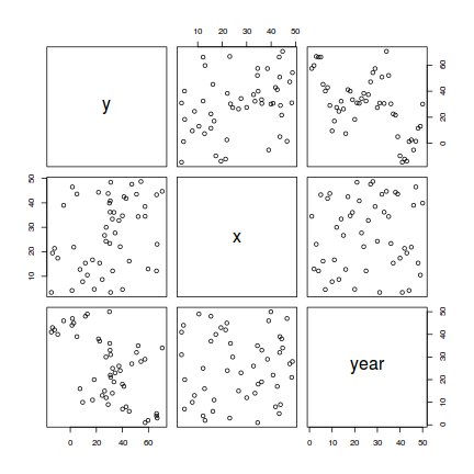
The above scatterplot suggests that the relationship between y and x (if it exists) is subtle. The observations have been collected over time and the scatterplot also indicates a relationship between y and year. This later trend (y drifting over time) could make detecting an effect of x difficult.
Standard regression modelling assumes that all residuals are independent. When they are not independent, standard errors of parameter estimates from standard regression modelling will be biased and unreliable. The trend of y over year suggests that observations (and thus residuals) that are collected closer together in time are likely to be more similar to one another than they are to observations collected further apart in time.
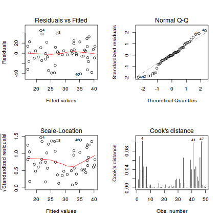
Lets start by fitting a simple linear regression model, and exploring the model fitting diagnostics.
data.temporalCor.lm <- lm(y ~ x, data = data.temporalCor)
par(mfrow = c(2, 2))
plot(data.temporalCor.lm, which = 1:4)
plot(rstandard(data.temporalCor.lm) ~ data.temporalCor$x)
plot(rstandard(data.temporalCor.lm) ~ data.temporalCor$year)
abline(h = 0, lty = 2)
lines(rstandard(data.temporalCor.lm) ~ data.temporalCor$year)
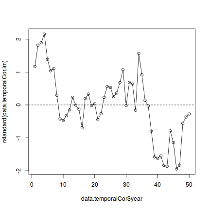
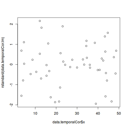
Conclusions - there is clearly a pattern in the residuals that relates to year.
Given that the observations were collected over time, it is worth exploring whether there is any suggestion of temporal autocorrelation in the residuals. The code below plots the results of the acf() function that calculates the degree of correlation associated with increasing lags. Hence at a lag of 0, the acf() function calculates the degree of correlation between the residuals and themselves. Obviously this will always be a correlation of 1. The correlation associated with a lag of 1 represents the correlation of the residual values with the residual values shifted forward one time unit. Hence, each lag represents the correlation of residual values with the same values shifted according to the lag.
When there is no autocorrelation in the residuals, the correlations associated with lags other than 0 should all be close to 0. When autocorrelation is present, the degree of correlation will show a pattern across lags. Typically, the correlations will start high (with low lag) and gradually decline. When there are cyclical patterns in the residuals, the correlations will also show some form of oscillation around zero correlation. In the acf() used below, the lag=40 argument is used to indicate the maximum lag to explore.
The autocorrelation plot displays the correlation against lag. Dashed horizontal lines indicate the boundaries of what correlations are not considered as significant.
plot(acf(rstandard(data.temporalCor.lm), lag = 40))
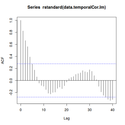
Conclusions - indeed there is evidence.
There are numerous causes of autocorrelation. One possibility is a misformed model. Perhaps the model is too simplistic and the addition of other predictors might address the issue. Usually when a plot of residuals against a unmodeled predictors reveal a pattern (as was the case above when plotting the residuals against year), it is a good idea to include that predictor in the model.
So lets incorporate, year into the linear model. Prior to fitting a multiple regression model we need to confirm that there is no collinearity between the covariates.
library(car)
vif(lm(y ~ x + year, data.temporalCor))
       x     year
1.002211 1.002211
Lets now fit the multiple linear regression model. And explore the diagnostics
data.temporalCor.lm1 <- lm(y ~ x + year, data.temporalCor)
par(mfrow = c(2, 2))
plot(data.temporalCor.lm1, which = 1:4)
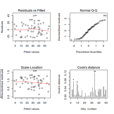
As before, we should explore all of the model fit diagnostics.
plot(rstandard(data.temporalCor.lm1) ~ data.temporalCor$x)
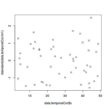
plot(rstandard(data.temporalCor.lm1) ~ data.temporalCor$year)
abline(h = 0, lty = 2)
lines(rstandard(data.temporalCor.lm1) ~ data.temporalCor$year)
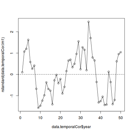
acf(rstandard(data.temporalCor.lm1), lag = 40)
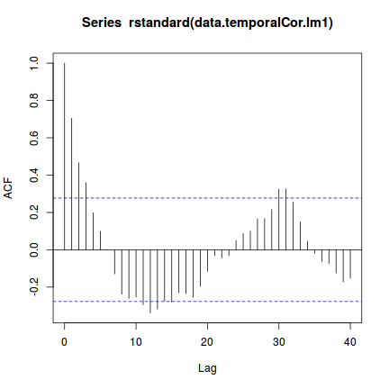
Modelling for temporal autocorrelation
As indicated earlier, observations collected closer together in time have a strong likelihood of being more closely correlated to one another - particularly when we know that y does change over time.
In the introduction to dealing with non-independence, I introduced one variance-covariance structure (compound symmetry) that did not assume zero covariance between residuals. However, for temporal auto-correlation (such as that depicted by the above auto-correlation plot), usually a more useful variance-covariance structure is one built around an auto-correlation structure.
The first order auto-regressive (AR1) structure defines a correlation structure in which the degree of correlation between two observations (or residuals) is proportional to the relative amount of elapsed time. Specifically, the correlation between two residuals is defined as $\rho^{|t-s|}$ where $|t-s|$ is the absolute difference between the current time ($t$) and the previous time ($s$). So if the correlation between two consecutive time periods is $\rho^1=\rho$ then the correlation for a lag of 2 is $\rho^2$ and so on.
$$ cor(\varepsilon) = \underbrace{ \begin{pmatrix} 1&\rho&\cdots&\rho^{|t-s|}\\ \rho&1&\cdots&\vdots\\ \vdots&\cdots&1&\vdots\\ \rho^{|t-s|}&\cdots&\cdots&1\\ \end{pmatrix}}_\text{First order autoregressive correlation structure} $$Modelling a first order autocorrelation only requires the estimation of a single additional parameter ($\rho$ - although often referred to as phi in output) as the decline in correlation is assumed to follow a very specific pattern (exponentially). This also assumes that the pattern of correlation decline depends only on the lag and not when in the time series the lag occurs. This is referred to as stationarity. Whilst this assumption does afford the analyses a large degree of simplicity, it might come at the cost of being too simplistic for complex temporal patterns.
Lets then incorporate this first order autoregressive structure into the model. To do so, we have to switch to gls() and use the correlation= argument. In addition to the model incorporating a first-order auto-regressive structure, we will refit the model with no correlation structure with the gls() function so that we can directly compare the fits of the two models.
To assist with comparisons, I will refit a model without temporal autocorrelation (left side) and a model with AR1 on the right. Both are fit with gls(). Using the correlation=corAR1() argument, we can indicate that the off-diagonals of the variance-covariance matrix should follow a specific pattern in which the degree of correlaton varies as an exponent equal to the lag. The spacing of the lags is taken from the form= argument. Of course, conceptually this is much more straight forward. If this is left blank, then it is assumed that the data are in chronological order and that each row represents a single unit increase in time (lag). In this case, the year variable is just a vector containing integers from 1 to 50, and therefore not strictly required. Nevertheless, it is good practice to always include it.
# Fit model data.temporalCor.gls1 = gls(y ~ x, data = data.temporalCor) # explore residuals plot(resid(data.temporalCor.gls1, type = "normalized") ~ fitted(data.temporalCor.gls1)) 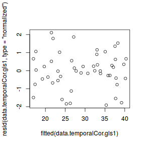 plot(resid(data.temporalCor.gls1, type = "normalized") ~ data.temporalCor$x) 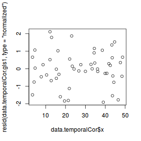 plot(resid(data.temporalCor.gls1, type = "normalized") ~ data.temporalCor$year) abline(h = 0, lty = 2) lines(resid(data.temporalCor.gls1, type = "normalized") ~ data.temporalCor$year) 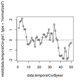 acf(residuals(data.temporalCor.gls1, type = "normalized"), lag = 40) 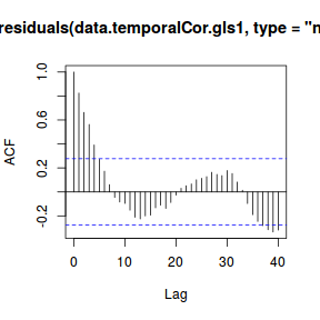 |
# Fit AR(1) model data.temporalCor.gls2 = gls(y ~ x, data = data.temporalCor, correlation = corAR1(form = ~year)) # explore residuals plot(resid(data.temporalCor.gls2, type = "normalized") ~ fitted(data.temporalCor.gls2)) 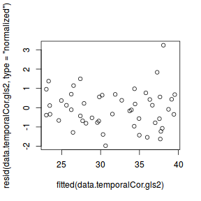 plot(resid(data.temporalCor.gls2, type = "normalized") ~ data.temporalCor$x) 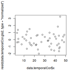 plot(resid(data.temporalCor.gls2, type = "normalized") ~ data.temporalCor$year) abline(h = 0, lty = 2) lines(resid(data.temporalCor.gls2, type = "normalized") ~ data.temporalCor$year) 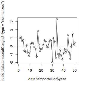 acf(residuals(data.temporalCor.gls2, type = "normalized"), lag = 40) 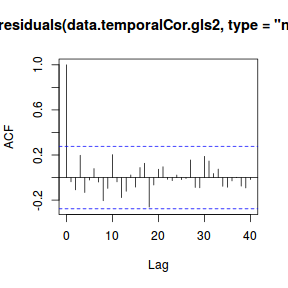 |
We can now compare the two models via AIC or a likelihood ratio test. Recall that when comparing the fit of models that differ in their random (variance-covariance) structure, the models must have been fit using REML (which is the default for gls).
AIC(data.temporalCor.gls1, data.temporalCor.gls2)
                      df      AIC
data.temporalCor.gls1  3 448.3029
data.temporalCor.gls2  4 387.6691
anova(data.temporalCor.gls1, data.temporalCor.gls2)
                      Model df      AIC      BIC    logLik   Test  L.Ratio p-value
data.temporalCor.gls1     1  3 448.3029 453.9165 -221.1515
data.temporalCor.gls2     2  4 387.6691 395.1539 -189.8346 1 vs 2 62.63378  <.0001
Normally, we would only then pursue this best model. However, for the purpose of this demonstration, it might be informative to compare the output and conclusions resulting from both models.
summary(data.temporalCor.gls1) Generalized least squares fit by REML
Model: y ~ x
Data: data.temporalCor
AIC BIC logLik
448.3029 453.9165 -221.1514
Coefficients:
Value Std.Error t-value p-value
(Intercept) 15.232510 6.435261 2.367039 0.0220
x 0.515328 0.209843 2.455776 0.0177
Correlation:
(Intr)
x -0.885
Standardized residuals:
Min Q1 Med Q3 Max
-1.91251132 -0.45316748 -0.01208734 0.60593126 2.11032351
Residual standard error: 21.14768
Degrees of freedom: 50 total; 48 residual
anova(data.temporalCor.gls1, type = "marginal") Denom. DF: 48
numDF F-value p-value
(Intercept) 1 5.602872 0.0220
x 1 6.030837 0.0177
|
summary(data.temporalCor.gls2) Generalized least squares fit by REML
Model: y ~ x
Data: data.temporalCor
AIC BIC logLik
387.6691 395.1539 -189.8346
Correlation Structure: AR(1)
Formula: ~year
Parameter estimate(s):
Phi
0.8793454
Coefficients:
Value Std.Error t-value p-value
(Intercept) 21.778167 11.868656 1.834931 0.0727
x 0.364699 0.086165 4.232586 0.0001
Correlation:
(Intr)
x -0.214
Standardized residuals:
Min Q1 Med Q3 Max
-1.8036769 -0.6122858 -0.1040566 0.3544122 1.6909436
Residual standard error: 23.60839
Degrees of freedom: 50 total; 48 residual
anova(data.temporalCor.gls2, type = "marginal") Denom. DF: 48
numDF F-value p-value
(Intercept) 1 3.366972 0.0727
x 1 17.914782 0.0001
|
Conclusions - The estimated AR(1) autocorrelation coefficient (Phi) is
0.8793454.
There are numerous differences between the two models.
- the estimated intercepts and slopes are quite different.
e standard errors are also quite different
Modelling for autocorrelation in the response
An alternative approach for relatively simple models is to say that if a residual associated with an observation is related to the residual from the observation from the previous time period, then we might be able to partly alleviate this by refitting the model by incorporating the residuals into the linear predictor.
mod = lm(y ~ x, data = data.temporalCor)
res = residuals(mod, type = "response")
dat = cbind(data.temporalCor, res) %>% mutate(epsilon = lag(res))
data.temporalCor.lm3 = lm(y ~ x + epsilon, data = dat)
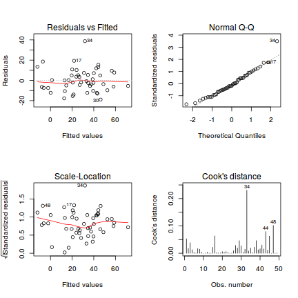
par(mfrow = c(2, 2))
plot(data.temporalCor.lm3, which = 1:4)
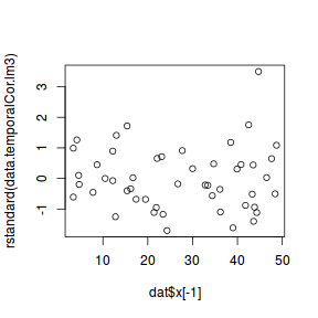
plot(rstandard(data.temporalCor.lm3) ~ dat$x[-1])
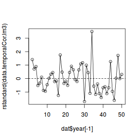
plot(rstandard(data.temporalCor.lm3) ~ dat$year[-1])
abline(h = 0, lty = 2)
lines(rstandard(data.temporalCor.lm3) ~ dat$year[-1])
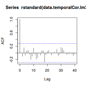
acf(rstandard(data.temporalCor.lm3), lag = 40)
summary(data.temporalCor.lm3)
Call:
lm(formula = y ~ x + epsilon, data = dat)

Residuals:
    Min      1Q  Median      3Q     Max
-18.945  -7.416  -2.002   7.134  38.718

Coefficients:
            Estimate Std. Error t value Pr(>|t|)
(Intercept) 19.21807    3.48247   5.519 1.52e-06 ***
x            0.34564    0.11409   3.030  0.00401 **
epsilon      0.84019    0.07832  10.727 4.17e-14 ***
---
Signif. codes:  0 '***' 0.001 '**' 0.01 '*' 0.05 '.' 0.1 ' ' 1

Residual standard error: 11.38 on 46 degrees of freedom
  (1 observation deleted due to missingness)
Multiple R-squared:  0.745,	Adjusted R-squared:  0.7339
F-statistic: 67.18 on 2 and 46 DF,  p-value: 2.251e-14
Cochran-Orcutt method
A modification of the above technique for estimating autocorrelation in simple regression applications was proposed by Cochran and Orcutt. They suggest that after estimating the first order autocorrelation parameter ($\rho$), the response and predictors are adjusted by subtracting the previous value multiplied by $\rho$ from the values and use these adjusted values in a regular regression.
mod = lm(y ~ x, data = data.temporalCor)
res = residuals(mod, type = "response")
(rho = sum(res[-length(res)] * res[-1])/sum(res^2))
[1] 0.8243546
# (rho=acf(res, plot=FALSE)$acf[2])
X = model.matrix(mod)
Y = y[-1] - y[-n] * rho
X = X[-1, ] - X[-n, ] * rho
summary(lm(Y ~ X - 1, corr = F))
Call:
lm(formula = Y ~ X - 1, corr = F)

Residuals:
    Min      1Q  Median      3Q     Max
-19.999  -7.204  -0.497   7.431  37.184

Coefficients:
             Estimate Std. Error t value Pr(>|t|)
X(Intercept) 16.02725    9.40639   1.704 0.095010 .
Xx            0.36341    0.08799   4.130 0.000148 ***
---
Signif. codes:  0 '***' 0.001 '**' 0.01 '*' 0.05 '.' 0.1 ' ' 1

Residual standard error: 11.18 on 47 degrees of freedom
Multiple R-squared:  0.3495,	Adjusted R-squared:  0.3219
F-statistic: 12.63 on 2 and 47 DF,  p-value: 4.079e-05
library(orcutt)
cochrane.orcutt(mod)
Cochrane-orcutt estimation for first order autocorrelation

Call:
lm(formula = y ~ x, data = data.temporalCor)

 number of interaction: 5
 rho 0.836316

Durbin-Watson statistic
(original):    0.32195 , p-value: 1.99e-15
(transformed): 2.02063 , p-value: 5.436e-01

 coefficients:
(Intercept)           x
  15.784493    0.363188
summary(cochrane.orcutt(mod))
Call:
lm(formula = y ~ x, data = data.temporalCor)

             Estimate Std. Error t value  Pr(>|t|)
(Intercept) 15.784493  10.044603   1.571 0.1227890
x            0.363188   0.087464   4.152 0.0001374 ***
---
Signif. codes:  0 '***' 0.001 '**' 0.01 '*' 0.05 '.' 0.1 ' ' 1

Residual standard error: 11.1725 on 47 degrees of freedom
Multiple R-squared:  0.2684 ,  Adjusted R-squared:  0.2528
F-statistic: 17.2 on 1 and 47 DF,  p-value: < 1.374e-04

Durbin-Watson statistic
(original):    0.32195 , p-value: 1.99e-15
(transformed): 2.02063 , p-value: 5.436e-01
