Tutorial 8.2a - Dealing with Heterogeneity
22 Jan 2018
Overview
The following representation of the standard linear model highlights the various assumptions that are imposed upon the underlying data. The current tutorial will focus directly on issues related to the nature of residual variability.

Dealing with heterogeneity (heteroskedasticity)
To reiterate, the validity and reliability of linear models are very much dependent on variance homogeneity. In particular, variances that increase (or decrease) with a change in expected values are substantial violations.
Whilst non-normality can also be a source of heterogeneity and therefore normalizing (or using an alternative distribution that might be better suited to the response) can address both issues, heterogeneity can also be independent of normality. Similarly for many response types, unequal variances might be expected. For example, the variance of count data (number of individuals per quadrat etc) tend to increase with increasing mean. When the expected number of individuals counted per quadrat is low (1, 2, 4,...), the variation in these counts is low. However, when the expected counts are high (100, 150, 250, ...), the expected variance of these counts is high.
Consequently, for many such situations it is arguably better to model the data against an error distribution better suited to the data (for example Poisson data is typically more suitable for count data than normal distribution). Generalized linear models (GLM) (that accommodate alternative residual distributions - such as Poisson, Binomial, Gamma etc) can be useful for more appropriate modelling of of both the distribution and variance of a model.
However, for Gaussian (normal) models in which there is evidence of heterogeneity of variance, yet no evidence of non-normality, it is also possible to specifically model in an alternative variance structure. For example, we can elect to allow variance to increase proportionally to a covariate.
To assist us in the following demonstration, we will generate another data set - one that has heteroscedasticity (unequal variance) by design. Rather than draw each residual (and thus observation) from a normal distribution with a constant standard deviation), we will draw the residuals from normal distributions whose variance is proportional to the X predictor.
set.seed(15)
n <- 16
a <- 40  #intercept
b <- 1.5  #slope
x <- 1:n  #values of the year covariate
sigma <- 1.5 * x
eps <- rnorm(n, mean = 0, sd = sigma)  #residuals
y <- a + b * x + eps  #response variable
# OR
y <- (model.matrix(~x) %*% c(a, b)) + eps
data.het <- data.frame(y = round(y, 1), x)  #dataset
head(data.het)  #print out the first six rows of the data set
     y x
1 41.9 1
2 48.5 2
3 43.0 3
4 51.4 4
5 51.2 5
6 37.7 6
# scatterplot of y against x
library(car)
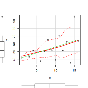
scatterplot(y ~ x, data.het)
# regular simple linear regression
data.het.lm <- lm(y ~ x, data.het)
# plot of standardized residuals
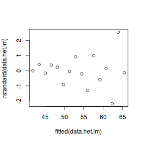
plot(rstandard(data.het.lm) ~ fitted(data.het.lm))
# plot of standardized residuals against the
# predictor
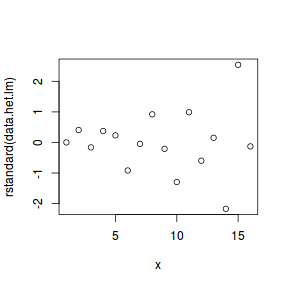
plot(rstandard(data.het.lm) ~ x)
- The above scatterplot suggests that variance may increase with increasing X.
- The residual plot (using standardized residuals) suggests that mean and variance could be related - there is more than a hint of a wedge-shaped pattern
- Importantly, the plot of standardized residuals against the predictor shows the same pattern as the residual plot implying that heterogeneity is likely to be due a relationship between variance and X. That is, an increase in X is associated with an increase in variance.
Weighted least squares (WLS)
In regular Ordinary Least Squares (OLS) parameter estimates assume that all observations are equally accurate, since we are assuming that all observations are drawn from populations that have the same variance. One way to tackle the issue of unequal variance is to alter the assumption of equal contribution of all observations, by weighting each observation differently. Specifically, we could put more weight (influence) on the observations drawn from low variance populations and less weight on those observations that are drawn from more varied populations.
However, given that we often only have a single observation associated with each predictor value (in simple regression anyway), how do we obtain estimates of how varied the populations from which the observations have been drawn are likely to be? There are two broad options:
- rather than assume all populations are equal, we might suspect that variance is in some way related to the magnitude of the predictor. For example, if we were attempting to establish a relationship between fish age and length (where length was the predictor of age), we might expect that as fish length increases, the range of likely ages also increases. Hence we might suggest that the variance in age is proportional to fish length. Consequently, when fitting a model, we might apply weights that are the inverse of the fish lengths.
- in the absence of a theoretical relationshop between variance and predictor, we could alternatively estimate the variances likely associated with each observations by fitting a regular regression model and using the residuals to estimate the associated variances to use as weights in a refit of the model.
Both of the above options are example of Weighted Least Squares (WLS) regression.
Specific relationship between variance and predictor
# weights
1/data.het$x
 [1] 1.00000000 0.50000000 0.33333333 0.25000000
 [5] 0.20000000 0.16666667 0.14285714 0.12500000
 [9] 0.11111111 0.10000000 0.09090909 0.08333333
[13] 0.07692308 0.07142857 0.06666667 0.06250000
data.het.lm1 = lm(y ~ x, weights = 1/x, data = data.het)
plot(rstandard(data.het.lm1) ~ fitted(data.het.lm1))
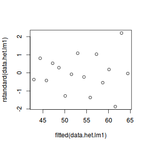
This is definitely an improvement.
To see what impact we had on the modelling outcome, we can contrast the estimates and standard errors of both OLS and WLS models.
summary(data.het.lm)
Call:
lm(formula = y ~ x, data = data.het)

Residuals:
     Min       1Q   Median       3Q      Max
-27.4203  -4.0197  -0.3129   4.8474  31.4090

Coefficients:
            Estimate Std. Error t value Pr(>|t|)
(Intercept)  40.3300     7.1894   5.610 6.44e-05
x             1.5707     0.7435   2.113   0.0531

(Intercept) ***
x           .
---
Signif. codes:
0 '***' 0.001 '**' 0.01 '*' 0.05 '.' 0.1 ' ' 1

Residual standard error: 13.71 on 14 degrees of freedom
Multiple R-squared:  0.2417,	Adjusted R-squared:  0.1876
F-statistic: 4.463 on 1 and 14 DF,  p-value: 0.05308
AIC(data.het.lm) [1] 133.0489 |
summary(data.het.lm1)
Call:
lm(formula = y ~ x, data = data.het, weights = 1/x)

Weighted Residuals:
   Min     1Q Median     3Q    Max
-7.125 -1.740 -0.223  2.292  8.342

Coefficients:
            Estimate Std. Error t value Pr(>|t|)
(Intercept)  41.5042     3.3323  12.455 5.79e-09
x             1.4326     0.5254   2.727   0.0164

(Intercept) ***
x           *
---
Signif. codes:
0 '***' 0.001 '**' 0.01 '*' 0.05 '.' 0.1 ' ' 1

Residual standard error: 4.079 on 14 degrees of freedom
Multiple R-squared:  0.3469,	Adjusted R-squared:  0.3002
F-statistic: 7.435 on 1 and 14 DF,  p-value: 0.01638
AIC(data.het.lm1) [1] 124.9284 |
Yep a definite improvement. By reducing some of the unexplained variability (some is explained by its relationship to $X$), we get a more powerful test.
Estimate variability from model
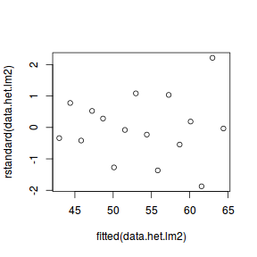
wts <- 1/fitted(lm(abs(residuals(data.het.lm)) ~ data.het$x))
data.het.lm2 = lm(y ~ x, data = data.het, weights = wts)
plot(rstandard(data.het.lm2) ~ fitted(data.het.lm2))
summary(data.het.lm2)
Call:
lm(formula = y ~ x, data = data.het, weights = wts)

Weighted Residuals:
    Min      1Q  Median      3Q     Max
-6.9806 -1.6820 -0.2159  2.1869  8.1851

Coefficients:
            Estimate Std. Error t value Pr(>|t|)
(Intercept)   41.528      3.497  11.876 1.07e-08
x              1.430      0.535   2.673   0.0182

(Intercept) ***
x           *
---
Signif. codes:
0 '***' 0.001 '**' 0.01 '*' 0.05 '.' 0.1 ' ' 1

Residual standard error: 3.982 on 14 degrees of freedom
Multiple R-squared:  0.3378,	Adjusted R-squared:  0.2905
F-statistic: 7.143 on 1 and 14 DF,  p-value: 0.01821
AIC(data.het.lm2)
[1] 125.2013
In this case, the outcome is almost identical to that when we assumed a specific relationship between variance and $X$. However, this is simply because the simulated data were generated with this very relationship.
Generalized least squares
In response to this, we could incorporate an alternative variance structure. The simple model we fit earlier assumed that the expected values were all drawn from normal distributions with the same level of variance ($\sigma^2$). $$ \mathbf{V} = cov = \underbrace{ \begin{pmatrix} \sigma^2&0&0&0&0&0&0&0&0&0&0&0&0&0&0\\ 0&\sigma^2&0&0&0&0&0&0&0&0&0&0&0&0&0\\ 0&0&\sigma^2&0&0&0&0&0&0&0&0&0&0&0&0\\ 0&0&0&\sigma^2&0&0&0&0&0&0&0&0&0&0&0\\ 0&0&0&0&\sigma^2&0&0&0&0&0&0&0&0&0&0\\ 0&0&0&0&0&\sigma^2&0&0&0&0&0&0&0&0&0\\ 0&0&0&0&0&0&\sigma^2&0&0&0&0&0&0&0&0\\ 0&0&0&0&0&0&0&\sigma^2&0&0&0&0&0&0&0\\ 0&0&0&0&0&0&0&0&\sigma^2&0&0&0&0&0&0\\ 0&0&0&0&0&0&0&0&0&\sigma^2&0&0&0&0&0\\ 0&0&0&0&0&0&0&0&0&0&\sigma^2&0&0&0&0\\ 0&0&0&0&0&0&0&0&0&0&0&\sigma^2&0&0&0\\ 0&0&0&0&0&0&0&0&0&0&0&0&\sigma^2&0&0\\ 0&0&0&0&0&0&0&0&0&0&0&0&0&\sigma^2&0\\ 0&0&0&0&0&0&0&0&0&0&0&0&0&0&\sigma^2\\ \end{pmatrix}}_\text{Variance-covariance matrix} $$ Which is often summarized as: $$ \mathbf{V} = \sigma^2\times \underbrace{ \begin{pmatrix} 1&0&\cdots&0\\ 0&1&\cdots&\vdots\\ \vdots&\cdots&1&\vdots\\ 0&\cdots&\cdots&1\\ \end{pmatrix}}_\text{Identity matrix} = \underbrace{ \begin{pmatrix} \sigma^2&0&\cdots&0\\ 0&\sigma^2&\cdots&\vdots\\ \vdots&\cdots&\sigma^2&\vdots\\ 0&\cdots&\cdots&\sigma^2\\ \end{pmatrix}}_\text{Variance-covariance matrix} $$ However, rather than assume that each observation is drawn from a normal distribution with the same amount of variance, we could alternatively assume that the variance is proportional to the level of the covariate. For mathematical reasons, it actually makes more sense that variance be inversely proportional to the square-root of the covariate values (we want more extreme observations to have less influence). $$ \mathbf{V} = \sigma^2\times X\times \underbrace{ \begin{pmatrix} 1&0&\cdots&0\\ 0&1&\cdots&\vdots\\ \vdots&\cdots&1&\vdots\\ 0&\cdots&\cdots&1\\ \end{pmatrix}}_\text{Identity matrix} = \underbrace{ \begin{pmatrix} \sigma^2\times \frac{1}{\sqrt{X_1}}&0&\cdots&0\\ 0&\sigma^2\times \frac{1}{\sqrt{X_2}}&\cdots&\vdots\\ \vdots&\cdots&\sigma^2\times \frac{1}{\sqrt{X_i}}&\vdots\\ 0&\cdots&\cdots&\sigma^2\times \frac{1}{\sqrt{X_n}}\\ \end{pmatrix}}_\text{Variance-covariance matrix} $$
Hence, what we are really doing is multiplying $\sigma^2$ by a matrix of weights ($\omega$): $$ \mathbf{V} = \sigma^2\times \omega, \hspace{1cm} \text{where } \omega = \underbrace{ \begin{pmatrix} \frac{1}{\sqrt{X_1}}&0&\cdots&0\\ 0&\frac{1}{\sqrt{X_2}}&\cdots&\vdots\\ \vdots&\cdots&\frac{1}{\sqrt{X_i}}&\vdots\\ 0&\cdots&\cdots&\frac{1}{\sqrt{X_n}}\\ \end{pmatrix}}_\text{Weights matrix} $$
Incorporating different variance structures into a linear model
In R, alternative variance structures are incorporated by specifying model weights. So we can re-write out the model as:
$$ \begin{align*} y_{i} &= \beta_0 + \beta_1 \times x_{i} + \varepsilon_i \hspace{1cm} &\epsilon_i\sim\mathcal{N}(0, \sigma^2) \\ y_{i} &= \beta_0 + \beta_1 \times x_{i} + \varepsilon_i \hspace{1cm} &\epsilon_i\sim\mathcal{N}(0, \sigma^2\times\omega) \\ \end{align*} $$
We will start by refitting the linear model incorporating weights that indicate that the variance is fixed to be proportional to X. Since the values of x are 1,2,3,4,5,6,7,8,9,10,11,12,13,14,15, the a fixed variance structure would be: $$ \mathbf{V} = cov = \sigma^2 \times \underbrace{ \begin{pmatrix} \frac{1}{\sqrt{1}}&0&0&0&0&0&0&0&0&0&0&0&0&0&0\\ 0&\frac{1}{\sqrt{2}}&0&0&0&0&0&0&0&0&0&0&0&0&0\\ 0&0&\frac{1}{\sqrt{3}}&0&0&0&0&0&0&0&0&0&0&0&0\\ 0&0&0&\frac{1}{\sqrt{4}}&0&0&0&0&0&0&0&0&0&0&0\\ 0&0&0&0&\frac{1}{\sqrt{5}}&0&0&0&0&0&0&0&0&0&0\\ 0&0&0&0&0&\frac{1}{\sqrt{6}}&0&0&0&0&0&0&0&0&0\\ 0&0&0&0&0&0&\frac{1}{\sqrt{7}}&0&0&0&0&0&0&0&0\\ 0&0&0&0&0&0&0&\frac{1}{\sqrt{8}}&0&0&0&0&0&0&0\\ 0&0&0&0&0&0&0&0&\frac{1}{\sqrt{9}}&0&0&0&0&0&0\\ 0&0&0&0&0&0&0&0&0&\frac{1}{\sqrt{10}}&0&0&0&0&0\\ 0&0&0&0&0&0&0&0&0&0&\frac{1}{\sqrt{11}}&0&0&0&0\\ 0&0&0&0&0&0&0&0&0&0&0&\frac{1}{\sqrt{12}}&0&0&0\\ 0&0&0&0&0&0&0&0&0&0&0&0&\frac{1}{\sqrt{13}}&0&0\\ 0&0&0&0&0&0&0&0&0&0&0&0&0&\frac{1}{\sqrt{14}}&0\\ 0&0&0&0&0&0&0&0&0&0&0&0&0&0&\frac{1}{\sqrt{15}}\\ \end{pmatrix}}_\text{Weights matrix} $$
Hence the weights are:
# calculate the weights
(wts <- 1/sqrt(data.het$x))
 [1] 1.0000000 0.7071068 0.5773503 0.5000000
 [5] 0.4472136 0.4082483 0.3779645 0.3535534
 [9] 0.3333333 0.3162278 0.3015113 0.2886751
[13] 0.2773501 0.2672612 0.2581989 0.2500000
However, to incorporate this properly into a linear model, we need to swap from the simple lm() (linear models via ordinary least squares) function to a linear modelling engine based on generalized least squares.
Generalized least squares (GLS) is a routine that uses ordinary least squares (OLS) to obtain estimates of the fixed effects parameters and then uses these estimates to generate maximum likelihood (ML) estimates of the variance parameters which in turn are used to update estimates of the fixed effects parameters. Unlike OLS, which assumes equal variance and zero correlation, GLS allows us to offer a variance-covariance structure for the model fit and is thus suitable for dealing with heteroscadacity and dependency issues.
Maximum likelihood (ML, that maximizes the likelihood of the data given the parameters) estimates of random effects parameters (including residual variance) are biased when sample sizes are small (although it is not clear how small is 'small'). Essentially the ML estimates are the sum of squares of residuals divided by the sample size. This is anti-conservative (small) as it does not account for the need to estimate fixed parameters (which uses some degrees of freedom).
An alternative to ML is restricted or residual maximum likelihood (REML). REML maximizes the likelihood of the residuals (rather than data) and therefore takes into account the number of estimated fixed parameters (equivalent to dividing residual sums of squares by the sample size minus the number of fixed effects parameters). Whilst REML yields unbiased random effects parameter estimates, REML models differing in fixed effects cannot be compared via log-likelihood ratio tests or information criteria (such as AIC). For relatively simple regression models, the gls() function in the nlme package is sufficient.
library(nlme)
summary(gls(y ~ x, data.het))
Generalized least squares fit by REML
  Model: y ~ x
  Data: data.het
       AIC      BIC    logLik
  127.6388 129.5559 -60.81939

Coefficients:
               Value Std.Error  t-value p-value
(Intercept) 40.33000  7.189442 5.609615  0.0001
x            1.57074  0.743514 2.112582  0.0531

 Correlation:
  (Intr)
x -0.879

Standardized residuals:
        Min          Q1         Med          Q3
-2.00006105 -0.29319830 -0.02282621  0.35357567
        Max
 2.29099872

Residual standard error: 13.70973
Degrees of freedom: 16 total; 14 residual
data.het.gls <- gls(y ~ x, data = data.het, weights = varFixed(~x),
    method = "REML")
Now we will have a look at the weights that were applied (these are stored in the fitted model). Fixed weights are just the inverse of the square-root of the covariate (x).
# the model weights used are stored in the model
attr(data.het.gls$model$varStruct, "weights")
 [1] 1.0000000 0.7071068 0.5773503 0.5000000
 [5] 0.4472136 0.4082483 0.3779645 0.3535534
 [9] 0.3333333 0.3162278 0.3015113 0.2886751
[13] 0.2773501 0.2672612 0.2581989 0.2500000
# the model weights are the inverse of the
# variances
1/attr(data.het.gls$model$varStruct, "weights")
 [1] 1.000000 1.414214 1.732051 2.000000 2.236068
 [6] 2.449490 2.645751 2.828427 3.000000 3.162278
[11] 3.316625 3.464102 3.605551 3.741657 3.872983
[16] 4.000000
# or we could express these in standard deviation
# units
(1/attr(data.het.gls$model$varStruct, "weights"))^2
 [1]  1  2  3  4  5  6  7  8  9 10 11 12 13 14 15
[16] 16
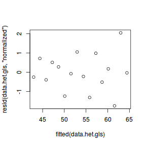
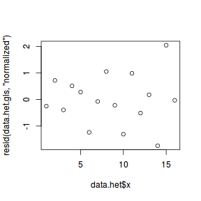
Fitting a linear model (earlier) that assumed homogeneity of variance yielded clear wedge shaped standardized residuals. Hence we should once again explore the standardized residuals to evaluate the fit of the generalized least squares model.
plot(resid(data.het.gls, "normalized") ~ fitted(data.het.gls))
plot(resid(data.het.gls, "normalized") ~ data.het$x)
At this point we should compare the fit of the above model to that of a model that assumes variance homogeneity. AIC would seem an appropriate metric to use for such a comparison. Recall that in order to compare models that differ in random structure, the models must be fitted with REML (which is the default but still declaring explicitly to ensure the code is clear on this point).
data.het.gls1 <- gls(y ~ x, data.het, method = "REML")
data.het.gls2 <- gls(y ~ x, data.het, weights = varFixed(~x),
    method = "REML")
AIC(data.het.gls1, data.het.gls2)
              df      AIC
data.het.gls1  3 127.6388
data.het.gls2  3 121.0828
121.0828432 vs 127.6387727),
it is arguably a more appropriate.
It is also possible to compare the two models via ANOVA. This is effectively testing the hypothesis: $$H_0: \sigma_1^2 = \sigma_2^2 = \sigma_3^2 = ... = \sigma^2$$ Since $\sigma^2$ is bounded at the lower end by 0 (values cannot be lower than zero), such a hypothesis test is said to be testing at the boundary and the p-values are likely to be conservative. Many recommend halving the p-values to compensate.
ANOVA can only compare like models. Thus in order to compare a model with two alternative variance functions, they need to be fitted with the same algorithms. In this case, it means that we need to fit the simple model again, this time with the gls function.
anova(data.het.gls1, data.het.gls2, test = TRUE)
              Model df      AIC      BIC
data.het.gls1     1  3 127.6388 129.5559
data.het.gls2     2  3 121.0828 123.0000
                 logLik
data.het.gls1 -60.81939
data.het.gls2 -57.54142
To see what impact we had on the modelling outcome, we can contrast the estimates and standard errors of both models. Be sure to use REML.
summary(data.het.lm)
Call:
lm(formula = y ~ x, data = data.het)

Residuals:
     Min       1Q   Median       3Q      Max
-27.4203  -4.0197  -0.3129   4.8474  31.4090

Coefficients:
            Estimate Std. Error t value Pr(>|t|)
(Intercept)  40.3300     7.1894   5.610 6.44e-05
x             1.5707     0.7435   2.113   0.0531

(Intercept) ***
x           .
---
Signif. codes:
0 '***' 0.001 '**' 0.01 '*' 0.05 '.' 0.1 ' ' 1

Residual standard error: 13.71 on 14 degrees of freedom
Multiple R-squared:  0.2417,	Adjusted R-squared:  0.1876
F-statistic: 4.463 on 1 and 14 DF,  p-value: 0.05308
|
summary(data.het.gls) Generalized least squares fit by REML
Model: y ~ x
Data: data.het
AIC BIC logLik
121.0828 123 -57.54142
Variance function:
Structure: fixed weights
Formula: ~x
Coefficients:
Value Std.Error t-value p-value
(Intercept) 41.50423 3.332272 12.455235 0.0000
x 1.43259 0.525383 2.726754 0.0164
Correlation:
(Intr)
x -0.746
Standardized residuals:
Min Q1 Med Q3
-1.74684117 -0.42652797 -0.05467358 0.56196012
Max
2.04502655
Residual standard error: 4.078973
Degrees of freedom: 16 total; 14 residual
|
Conclusion: the estimate of slope in the model incorporating the fixed variance structure is slightly lower than that of the model that assumes equal variance. Importantly, the estimated parameter standard errors of the former model are substantially lower. In this particular case, the more appropriate variance structure also lead to a change in conclusion. That is, the null hypothesis of no relationship between y and x would be rejected based on the GLS model, yet not based on the LM model.
Heteroscadacity in ANOVA
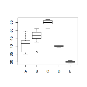
For regression models that include a categorical variable (e.g. ANOVA), heterogeneity manifests as vastly different variances for different levels (treatment groups) of the categorical variable. Recall, that this is diagnosed from the relative size of boxplots. Whilst, the degree of group variability may not be related to the means of the groups, having wildly different variances does lead to an increase in standard errors and thus a lowering of power.
In such cases, we would like to be able to indicate that the variances should be estimated separately for each group. That is the variance term is multiplied by a different number for each group. The appropriate matrix is referred to as an Identity matrix.
Again, to assist in the explanation some fabricated ANOVA data - data that has heteroscadasticity by design - will be useful.
set.seed(1)
ngroups <- 5  #number of populations
nsample <- 10  #number of reps in each
pop.means <- c(40, 45, 55, 40, 30)  #population mean length
sigma <- rep(c(6, 4, 2, 0.5, 1), each = nsample)  #residual standard deviation
n <- ngroups * nsample  #total sample size
eps <- rnorm(n, 0, sigma)  #residuals
x <- gl(ngroups, nsample, n, lab = LETTERS[1:5])  #factor
means <- rep(pop.means, rep(nsample, ngroups))
X <- model.matrix(~x - 1)  #create a design matrix
y <- as.numeric(X %*% pop.means + eps)
data.het1 <- data.frame(y, x)
boxplot(y ~ x, data.het1)
plot(lm(y ~ x, data.het1), which = 3)
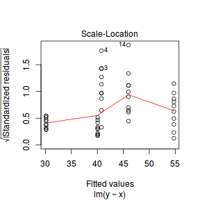
It is clear that there is gross heteroscedasticity. The residuals are obviously more spread in some groups than others yet there is no real pattern with means (the residual plot does not show an obvious wedge). Note, for assessing homogeneity of variance, it is best to use the standardized residuals.
It turns out that if we switch over to maximum (log) likelihood estimation methods, we can model in a within-group heteroscedasticity structure rather than just assume one very narrow form of variance structure.
Lets take a step back and reflect on our simple ANOVA (regression) model that has five groups each with 10 observations: $$y = \mu + \alpha_i + \varepsilon, \quad \varepsilon \sim \mathcal{N}(0,\sigma^2)$$ This is shorthand notation to indicate that the response variable is being modelled against a specific linear predictor and that the residuals follow a normal distribution with a certain variance (that is the same for each group).
Rather than assume that the variance of each group is the same, we could relax this a little so as to permit different levels of variance per group: $$\varepsilon \sim \mathcal{N}(0,\sigma_i^2)$$
To achieve this, we actually multiply the variance matrix by a weighting matrix, where the weights associated with each group are determined by the inverse of the ratio of each group to the first (reference) group: $$\varepsilon \sim \mathcal{N}(0,\sigma_i^2\times \omega)$$
So returning to our five groups of 10 observations example, the weights would be determined as:
data.het1.sd <- with(data.het1, tapply(y, x, sd))
1/(data.het1.sd[1]/data.het1.sd)
         A          B          C          D
1.00000000 0.91342905 0.40807277 0.08632027
         E
0.12720488
In order to incorporate these weights, we need to shift over to a different linear modelling function (gls within the nlme package). This function fits analogous models to lm(), yet allows us to describe the within-group heteroscedasticity and correlation structure.
library(nlme)
# Fit the standard linear model (assuming homogeneity of variances)
data.het1.gls <- gls(y ~ x, data = data.het1, method = "REML")
# Fit a linear model with different relative variance weights for each group.
data.het1.gls1 <- gls(y ~ x, data = data.het1, weights = varIdent(form = ~1 | x), method = "REML")
To determine whether allowing for separate variances per group is worth the extra degrees of freedom it costs, we can either:
- compare the fit of the two models (with and without separate variances)
- investigate the following hypothesis (that the variances of each groups are equal): $$\text{H}_0: \sigma_1^2 = \sigma_2^2 = \sigma_3^2 = \sigma_4^2 = \sigma_5^2 = \sigma^2$$
data.het1.gls2 <- update(data.het1.gls, method = "REML")
data.het1.gls3 <- update(data.het1.gls1, method = "REML")

AIC(data.het1.gls2, data.het1.gls3)
               df      AIC
data.het1.gls2  6 249.4968
data.het1.gls3 10 199.2087
anova(data.het1.gls2, data.het1.gls3, test = TRUE)
               Model df      AIC      BIC     logLik   Test  L.Ratio p-value
data.het1.gls2     1  6 249.4968 260.3368 -118.74841
data.het1.gls3     2 10 199.2087 217.2753  -89.60435 1 vs 2 58.28812  <.0001
Both approaches offer the same conclusion: that the model allowing separate variances per group is substantially better. We can further confirm this, by exploring the standardized residuals. Note that the model incorporating separate variances uses up more degrees of freedom (as it has to estimate multiple $\sigma^2$ rather than just a single one. Nevertheless, this is more than compensated by the additional explanatory power of the model fit.
plot(data.het1.gls1)

At this point, it might also be instruction to compare the two models (equal and separate variances) side by side:
summary(data.het1.gls) Generalized least squares fit by REML
Model: y ~ x
Data: data.het1
AIC BIC logLik
249.4968 260.3368 -118.7484
Coefficients:
Value Std.Error t-value p-value
(Intercept) 40.79322 0.9424249 43.28538 0.0000
xB 5.20216 1.3327901 3.90321 0.0003
xC 13.93944 1.3327901 10.45884 0.0000
xD -0.73285 1.3327901 -0.54986 0.5851
xE -10.65908 1.3327901 -7.99757 0.0000
Correlation:
(Intr) xB xC xD
xB -0.707
xC -0.707 0.500
xD -0.707 0.500 0.500
xE -0.707 0.500 0.500 0.500
Standardized residuals:
Min Q1 Med Q3 Max
-3.30653942 -0.24626108 0.06468242 0.39046918 2.94558782
Residual standard error: 2.980209
Degrees of freedom: 50 total; 45 residual
plot(data.het1.gls) 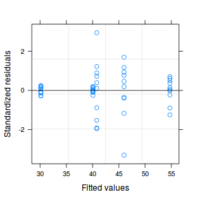 |
summary(data.het1.gls1) Generalized least squares fit by REML
Model: y ~ x
Data: data.het1
AIC BIC logLik
199.2087 217.2753 -89.60435
Variance function:
Structure: Different standard deviations per stratum
Formula: ~1 | x
Parameter estimates:
A B C D E
1.00000000 0.91342372 0.40807004 0.08631969 0.12720393
Coefficients:
Value Std.Error t-value p-value
(Intercept) 40.79322 1.481066 27.543153 0.0000
xB 5.20216 2.005924 2.593399 0.0128
xC 13.93944 1.599634 8.714142 0.0000
xD -0.73285 1.486573 -0.492981 0.6244
xE -10.65908 1.493000 -7.139371 0.0000
Correlation:
(Intr) xB xC xD
xB -0.738
xC -0.926 0.684
xD -0.996 0.736 0.922
xE -0.992 0.732 0.918 0.988
Standardized residuals:
Min Q1 Med Q3 Max
-2.3034240 -0.6178652 0.1064904 0.7596732 1.8743230
Residual standard error: 4.683541
Degrees of freedom: 50 total; 45 residual
plot(data.het1.gls1) 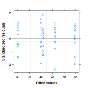 |
- Notice that allowing for separate variances per group has had no influence on the parameter estimates, only the standard deviation (and thus standard error) of these estimates. Note that each parameter has a unique standard error.
- The variance structure is provided for the separate variances - these are the weights.
A more thorough explanation
A more thorough explanation follows
However, a more accurate way of writing the model would be to use matrix or vector notation:
$$\mathbf{Y}_{i} \sim \mathcal{N}(\mathbf{X}_i\times \boldsymbol{\beta}, \mathbf{V}_{i})$$
In other words, the values of Y are expected to be drawn from a normal distribution with an expected value equal to the linear predictor
($\mathbf{X}_i\times \boldsymbol{\beta}$) and a standard deviation of V.
where $i$ denotes each of the groups and thus $V_i$ represents the variance matrix for associated with the observations of each of the groups.
Let us focus more on the $\varepsilon \sim \mathcal{N}(0,\sigma^2)$.
Actually, the $\sigma^2$ should really be
- normally distributed
- independent
- equally varied - note that in the above representation there is only a single $\sigma^2$ (variance) term. This implies that there is a single variance that represents the variance for each observation (and thus within each group).
The bold symbols represent:
- $\mathbf{X}$ - the model matrices for the data in each group. The first column of each matrix is a vector or 1's and then there are additional columns for each of the effects ($\alpha_2$, $\alpha_3$, ...).
- $\boldsymbol{\beta}_i$ - the regression parameter associated with $i^{th}$ group.
- $\mathbf{V}_i$ - the variance matrix for the observations within each of the $i$ groups
In the above variance-covariance matrix, all of the off-diagonals are 0. This reflects the independence assumption. That is
Other variance structures
It is also possible (though less common), that variance is non-linearly proportional to covariate - either exponentially or via a power function. To accommodate these situations there are also a couple of additional inbuilt variance functions available. Each of the available variance functions available are described in the following table:
| Variance function | Variance structure | Description |
|---|---|---|
| varFixed(~x) | $V = \sigma^2\times x$ | variance proportional to x the covariate |
| varExp(form=~x) | $V = \sigma^2\times e^{2\delta\times x}$ | variance proportional to the exponential of x multiplied by a constant |
| varPower(form=~x) | $V = \sigma^2\times |x|^{2\delta}$ | variance proportional to the absolute value of x raised to a constant power |
| varConstPower(form=~x) | $V = \sigma^2\times (\delta_1 + |x|^{\delta_2})^2$ | a variant on the power function |
| varIdent(form=~|A) | $V = \sigma_j^2\times I$ | when A is a factor, variance is allowed to be different for each level ($j$) of the factor |
| varComb(form=~x|A) | $V = \sigma_j^2\times x$ | combination of two of the above |
Finally, heterogeneity can also be caused by other underlying differences in the sampled populations that are otherwise not controlled for in the sampling design. For example, perhaps some other characteristic of the sampling units also changes with increasing X. In such situations, incorporating this other characteristic into the model as a covariate or using it as a model offset could help standardize for this effect and thus even up the variances.
