Tutorial 9.2b - Nested ANOVA (Bayesian)
23 Dec 2015
If you are completely ontop of the conceptual issues pertaining to Nested ANOVA, and just need to use this tutorial in order to learn about Nested ANOVA in R, you are invited to skip down to the section on Nested ANOVA in R.
Overview
You are strongly advised to review the information on the nested design in tutorial 9.2a. I am not going to duplicate the overview here.
Linear models
So called 'random effects' are modelled differently from 'fixed effects' in that rather than estimate their individual effects, we instead estimate the variability due to these 'random effects'. Since technically all variables in a Bayesian framework are random, some prefer to use the terms 'fixed effects' and 'varying effects'. As random factors typically represent 'random' selections of levels (such as a set of randomly selected sites), incorporated in order to account for the dependency structure (observations within sites are more likely to be correlated to one another - not strickly independent) to the data, we are not overly interested in the individual differences between levels of the 'varying' (random) factor. Instead (in addition to imposing a separate correlation structure within each nest), we want to know how much variability is attributed to this level of the design.
The linear models for two and three factor nested design are:
$$
\begin{align}
y_{ijk}&=\mu+\alpha_i + \beta_{j(i)} + \varepsilon_{ijk} &\hspace{2em} \varepsilon_{ijk}&\sim\mathcal{N}(0,\sigma^2), \hspace{1em}\beta_{j(i)}\sim\mathcal{N}(0,\sigma_B^2)\\
y_{ijkl}&=\mu+\alpha_i + \beta_{j(i)} + \gamma_{k(j(i))} + \varepsilon_{ijkl} &\hspace{2em} \varepsilon_{ijkl}&\sim\mathcal{N}(0,\sigma^2), \hspace{1em}\beta_{j(i)}\sim\mathcal{N}(0,\sigma_B^2), \hspace{1em}\gamma_{k(j(i))}\sim\mathcal{N}(0,\sigma_C^2)\\
\end{align}
$$
where $\mu$ is the overall mean, $\alpha$ is the effect of Factor A, $\beta$ is the variability of Factor B (nested within Factor A), $\gamma$ is the variability of Factor C (nested within Factor B) and $\varepsilon$ is the random unexplained or residual component that is assumed to be normally distributed with a mean of zero and a constant amount of standard deviation ($\sigma^2$).
The subscripts are iterators. For example, the $i$ represents the number of effects to be estimated for Factor A. Thus the first formula can be read as 'the $k$th observation of $y$ is drawn from a normal distribution (with a specific level of variability) and mean proposed to be determined by a base mean ($\mu$ - mean of the first treatment across all nests) plus the effect of the $i$th treatment effect plus the variability 'the model proposes that given a base mean ($\mu$) and knowing the effect of the $i$th treatment (factor A) and which of the $j$th nests within the treatment 'the $k$th observation from Block $j$ (factor B) within treatment effect
Variance components
As previously alluded to, it can often be useful to determine the relative contribution (to explaining the unexplained variability) of each of the factors as this provides insights into the variability at each different scales.
These contributions are known as Variance components and are estimates of the added variances due to each of the factors. For consistency with leading texts on this topic, I have included estimated variance components for various balanced nested ANOVA designs in the above table. However, variance components based on a modified version of the maximum likelihood iterative model fitting procedure (REML) is generally recommended as this accommodates both balanced and unbalanced designs.
While there are no numerical differences in the calculations of variance components for fixed and random factors, fixed factors are interpreted very differently and arguably have little biological meaning (other to infer relative contribution). For fixed factors, variance components estimate the variance between the means of the specific populations that are represented by the selected levels of the factor and therefore represent somewhat arbitrary and artificial populations. For random factors, variance components estimate the variance between means of all possible populations that could have been selected and thus represents the true population variance.
Assumptions
Consistent with the hierarchical nature of the design (in which the site means are the appropriate level of replication for the main treatments), it is important that diagnostics associated with each factor reflect this hierarchy. Hence, the replicates for the treatment effects are the site means, and the replicates of the sites are the quadrat means.
- All of the observations are independent - this must be addressed at the design and collection stages. Importantly, to be considered independent replicates, the replicates must be made at the same scale at which the treatment is applied. For example, if the experiment involves subjecting organisms housed in tanks to different water temperatures, then the unit of replication is the individual tanks not the individual organisms in the tanks. The individuals in a tank are strictly not independent with respect to the treatment.
- The response variable (and thus the residuals) should be normally distributed for each sampled populations (combination of factors). Boxplots of each treatment combination are useful for diagnosing major issues with normality.
- The response variable should be equally varied (variance should not be related to mean as these are supposed to be estimated separately) for each combination of treatments. Again, boxplots are useful.
Design balance
In a Bayesian framework, issues of design balance essentially evaporate.
Nested ANOVA in R
Scenario and Data
Imagine we has designed an experiment in which we intend to measure a response ($y$) to one of treatments (three levels; 'a1', 'a2' and 'a3'). The treatments occur at a spatial scale (over an area) that far exceeds the logistical scale of sampling units (it would take too long to sample at the scale at which the treatments were applied). The treatments occurred at the scale of hectares whereas it was only feasible to sample $y$ using 1m quadrats.
Given that the treatments were naturally occurring (such as soil type), it was not possible to have more than five sites of each treatment type, yet prior experience suggested that the sites in which you intended to sample were very uneven and patchy with respect to $y$.
In an attempt to account for this inter-site variability (and thus maximize the power of the test for the effect of treatment, you decided to employ a nested design in which 10 quadrats were randomly located within each of the five replicate sites per three treatments. As this section is mainly about the generation of artificial data (and not specifically about what to do with the data), understanding the actual details are optional and can be safely skipped. Consequently, I have folded (toggled) this section away.
- the number of treatments = 3
- the number of sites per treatment = 5
- the total number of sites = 15
- the sample size per treatment= 5
- the number of quadrats per site = 10
- the mean of the treatments = 40, 70 and 80 respectively
- the variability (standard deviation) between sites of the same treatment = 12
- the variability (standard deviation) between quadrats within sites = 5
library(plyr)
set.seed(1)
nTreat <- 3
nSites <- 15
nSitesPerTreat <- nSites/nTreat
nQuads <- 10
site.sigma <- 12
sigma <- 5
n <- nSites * nQuads
sites <- gl(n=nSites,k=nQuads, lab=paste0('S',1:nSites))
A <- gl(nTreat, nSitesPerTreat*nQuads, n, labels=c('a1','a2','a3'))
a.means <- c(40,70,80)
## the site means (treatment effects) are drawn from normal distributions
## with means of 40, 70 and 80 and standard deviations of 12
A.effects <- rnorm(nSites, rep(a.means,each=nSitesPerTreat),site.sigma)
#A.effects <- a.means %*% t(model.matrix(~A, data.frame(A=gl(nTreat,nSitesPerTreat,nSites))))+rnorm(nSites,0,site.sigma)
Xmat <- model.matrix(~sites -1)
lin.pred <- Xmat %*% c(A.effects)
## the quadrat observations (within sites) are drawn from
## normal distributions with means according to the site means
## and standard deviations of 5
y <- rnorm(n,lin.pred,sigma)
data.nest <- data.frame(y=y, A=A, Sites=sites,Quads=1:length(y))
head(data.nest)  #print out the first six rows of the data set
         y  A Sites Quads
1 32.25789 a1    S1     1
2 32.40160 a1    S1     2
3 37.20174 a1    S1     3
4 36.58866 a1    S1     4
5 35.45206 a1    S1     5
6 37.07744 a1    S1     6
library(ggplot2)
ggplot(data.nest, aes(y=y, x=1)) + geom_boxplot() + facet_grid(.~Sites)

Exploratory data analysis
Normality and Homogeneity of variance
#Effects of treatment
library(plyr)
boxplot(y~A, ddply(data.nest, ~A+Sites,numcolwise(mean, na.rm=T)))

#Site effects
boxplot(y~Sites, ddply(data.nest, ~A+Sites+Quads,numcolwise(mean, na.rm=T)))

## with ggplot2
ggplot(ddply(data.nest, ~A+Sites,numcolwise(mean, na.rm=T)), aes(y=y, x=A)) +
  geom_boxplot()

Conclusions:
- there is no evidence that the response variable is consistently non-normal across all populations - each boxplot is approximately symmetrical
- there is no evidence that variance (as estimated by the height of the boxplots) differs between the five populations. . More importantly, there is no evidence of a relationship between mean and variance - the height of boxplots does not increase with increasing position along the y-axis. Hence it there is no evidence of non-homogeneity
- transform the scale of the response variables (to address normality etc). Note transformations should be applied to the entire response variable (not just those populations that are skewed).
JAGS
For non-hierarchical linear models, uniform priors on variance (standard deviation) parameters seem to
work reasonably well.
Gelman (2006) warns that the use of the inverse-gamma family of non-informative
priors are very sensitive to $\epsilon$ particularly when variance is close to zero and this may lead to unintentionally
informative priors. When the number of groups (treatments or varying/random effects) is large (more than 5),
Gelman (2006) advocated the use of either uniform or half-cauchy priors. Yet when the
number of groups is low, Gelman (2006) indicates that uniform priors have a tendency
to result in inflated variance estimates. Consequently, half-cauchy priors are generally recommended for variances.
| Full parameterization | Matrix parameterization | Heirarchical parameterization |
|---|---|---|
| $$ \begin{array}{rcl} y_{ijk}&\sim&\mathcal{N}(\mu_{ij},\sigma^2)\\ \mu_{ij} &=& \alpha_0 + \alpha_{i} + \beta_{j(i)}\\ \beta_{i{j}}&\sim&\mathcal{N}(0,\sigma_{B}^2)\\ \alpha_0, \alpha_i&\sim&\mathcal{N}(0,100000)\\ \sigma^2, \sigma_{B}^2&\sim&\mathcal{Cauchy}(0,25)\\ \end{array} $$ | $$ \begin{array}{rcl} y_{ijk}&\sim&\mathcal{N}(\mu_{ij},\sigma^2)\\ \mu_{ij} &=& \alpha\mathbf{X} + \beta_{j(i)}\\ \beta_{i{j}}&\sim&\mathcal{N}(0,\sigma_{B}^2)\\ \alpha&\sim&\mathcal{MVN}(0,100000)\\ \sigma^2, \sigma_{B}^2&\sim&\mathcal{Cauchy}(0,25)\\ \end{array} $$ | $$ \begin{array}{rcl} y_{ij}&\sim &\mathcal{N}(\beta_{j(i)}, \sigma^2)\\ \beta_{j(i)}&\sim&\mathcal{N}(\mu_{i},\sigma_{B}^2)\\ \mu_{i}&=&\alpha\mathbf{X}\\ \alpha_i&\sim&\mathcal{N}(0, 1000000)\\ \sigma^2, \sigma_{B}^2&\sim&\mathcal{Cauchy}(0,25)\\ \end{array} $$ |
The full parameterization, shows the effects parameterization in which there is an intercept ($\alpha_0$) and two treatment effects ($\alpha_i$, where $i$ is 1,2).
The matrix parameterization is a compressed notation, In this parameterization, there are three alpha parameters (one representing the mean of treatment a1, and the other two representing the treatment effects (differences between a2 and a1 and a3 and a1). In generating priors for each of these three alpha parameters, we could loop through each and define a non-informative normal prior to each (as in the Full parameterization version). However, it turns out that it is more efficient (in terms of mixing and thus the number of necessary iterations) to define the priors from a multivariate normal distribution. This has as many means as there are parameters to estimate (3) and a 3x3 matrix of zeros and 100 in the diagonals. $$ \mu\sim\left[ \begin{array}{c} 0\\ 0\\ 0\\ \end{array} \right], \hspace{2em} \sigma^2\sim\left[ \begin{array}{ccc} 1000000&0&0\\ 0&1000000&0\\ 0&0&1000000\\ \end{array} \right] $$
In the Heirarchical parameterization, we are indicating two residual layers - one representing the variability in the observed data between individual observations (within sites) and the second representing the variability between site means (within the three treatments).
Full effects parameterization
modelString="
model {
   #Likelihood
   for (i in 1:n) {
      y[i]~dnorm(mu[i],tau)
      mu[i] <- alpha0 + alpha[A[i]] + beta[site[i]]
   }

   #Priors
   alpha0 ~ dnorm(0, 1.0E-6)
   alpha[1] <- 0
   for (i in 2:nA) {
     alpha[i] ~ dnorm(0, 1.0E-6) #prior
   }
   for (i in 1:nSite) {
     beta[i] ~ dnorm(0, tau.B) #prior
   }
   tau <- pow(sigma,-2)
   sigma <-z/sqrt(chSq)
   z ~ dnorm(0, .0016)I(0,)
   chSq ~ dgamma(0.5, 0.5)

   tau.B <- pow(sigma.B,-2)
   sigma.B <-z/sqrt(chSq.B)
   z.B ~ dnorm(0, .0016)I(0,)
   chSq.B ~ dgamma(0.5, 0.5)
 }
"
writeLines(modelString,con="../downloads/BUGSscripts/tut9.2bS3.1.f.txt")
data.nest.list <- with(data.nest,
        list(y=y,
                 site=as.numeric(Sites),
         A=as.numeric(A),
         n=nrow(data.nest),
         nSite=length(levels(Sites)),
                 nA = length(levels(A))
         )
)

params <- c("alpha0","alpha","sigma","sigma.B")
adaptSteps = 1000
burnInSteps = 3000
nChains = 3
numSavedSteps = 3000
thinSteps = 10
nIter = burnInSteps+ceiling((numSavedSteps * thinSteps)/nChains)

library(R2jags)
rnorm(1)
[1] -0.5428819
jags.effects.f.time <- system.time(
data.nest.r2jags.f <- jags(data=data.nest.list,
          inits=NULL,
          parameters.to.save=params,
          model.file="../downloads/BUGSscripts/tut9.2bS3.1.f.txt",
          n.chains=3,
          n.iter=nIter,
          n.burnin=burnInSteps,
      n.thin=thinSteps
          )
)
Compiling model graph
   Resolving undeclared variables
   Allocating nodes
   Graph Size: 503

Initializing model
jags.effects.f.time
   user  system elapsed
  7.812   0.008   7.874
print(data.nest.r2jags.f)
Inference for Bugs model at "../downloads/BUGSscripts/tut9.2bS3.1.f.txt", fit using jags,
 3 chains, each with 13000 iterations (first 3000 discarded), n.thin = 10
 n.sims = 3000 iterations saved
         mu.vect sd.vect    2.5%     25%     50%     75%   97.5%  Rhat n.eff
alpha[1]   0.000   0.000   0.000   0.000   0.000   0.000   0.000 1.000     1
alpha[2]  30.088   9.059  12.031  24.445  30.049  35.796  48.112 1.001  3000
alpha[3]  37.141   9.101  19.689  31.396  37.121  42.774  55.403 1.002  1700
alpha0    42.171   6.447  29.586  38.114  42.136  46.235  55.100 1.001  3000
sigma      4.428   0.273   3.940   4.241   4.415   4.598   4.996 1.001  3000
sigma.B   14.057   3.179   9.421  11.801  13.572  15.590  22.385 1.001  3000
deviance 869.642   6.183 859.552 865.156 868.846 873.323 883.745 1.002  1300

For each parameter, n.eff is a crude measure of effective sample size,
and Rhat is the potential scale reduction factor (at convergence, Rhat=1).

DIC info (using the rule, pD = var(deviance)/2)
pD = 19.1 and DIC = 888.7
DIC is an estimate of expected predictive error (lower deviance is better).
data.nest.mcmc.list.f <- as.mcmc(data.nest.r2jags.f)
[1] "alpha0" "alpha[1]" "alpha[2]" "alpha[3]" "deviance" "sigma" "sigma.B"
Matrix parameterization
modelString="
model {
   #Likelihood
   for (i in 1:n) {
      y[i]~dnorm(mu[i],tau)
      mu[i] <- inprod(alpha[],X[i,]) + beta[site[i]]
   }

   #Priors
   alpha ~ dmnorm(a0,A0)
   for (i in 1:nSite) {
     beta[i] ~ dnorm(0, tau.B) #prior
   }
   tau <- pow(sigma,-2)
   sigma <-z/sqrt(chSq)
   z ~ dnorm(0, .0016)I(0,)
   chSq ~ dgamma(0.5, 0.5)

   tau.B <- pow(sigma.B,-2)
   sigma.B <-z/sqrt(chSq.B)
   z.B ~ dnorm(0, .0016)I(0,)
   chSq.B ~ dgamma(0.5, 0.5)

 }
"
writeLines(modelString,con="../downloads/BUGSscripts/tut9.2bS3.1.m.txt")
A.Xmat <- model.matrix(~A,data.nest)
data.nest.list <- with(data.nest,
        list(y=y,
                 site=as.numeric(Sites),
         X=A.Xmat,
         n=nrow(data.nest),
         nSite=length(levels(Sites)),
                 nA = ncol(A.Xmat),
         a0=rep(0,3), A0=diag(0,3)
         )
)

params <- c("alpha","sigma","sigma.B")
adaptSteps = 1000
burnInSteps = 3000
nChains = 3
numSavedSteps = 3000
thinSteps = 10
nIter = burnInSteps+ceiling((numSavedSteps * thinSteps)/nChains)

library(R2jags)
rnorm(1)
[1] 0.79071
jags.effects.m.time <- system.time(
data.nest.r2jags.m <- jags(data=data.nest.list,
          inits=NULL,
          parameters.to.save=params,
          model.file="../downloads/BUGSscripts/tut9.2bS3.1.m.txt",
          n.chains=3,
          n.iter=nIter,
          n.burnin=burnInSteps,
      n.thin=thinSteps
          )
)
Compiling model graph
   Resolving undeclared variables
   Allocating nodes
   Graph Size: 965

Initializing model
jags.effects.m.time
   user  system elapsed
  9.577   0.008   9.670
print(data.nest.r2jags.m)
Inference for Bugs model at "../downloads/BUGSscripts/tut9.2bS3.1.m.txt", fit using jags,
 3 chains, each with 13000 iterations (first 3000 discarded), n.thin = 10
 n.sims = 3000 iterations saved
         mu.vect sd.vect    2.5%     25%     50%     75%   97.5%  Rhat n.eff
alpha[1]  42.362   6.448  29.963  38.129  42.351  46.617  54.771 1.003   900
alpha[2]  29.814   8.935  12.056  23.942  29.743  35.587  47.542 1.001  2300
alpha[3]  36.868   9.024  18.302  31.194  36.774  42.735  54.574 1.002  1400
sigma      4.431   0.270   3.945   4.242   4.417   4.603   5.009 1.001  2500
sigma.B   14.133   3.020   9.599  11.972  13.638  15.759  21.385 1.001  3000
deviance 869.516   5.925 860.027 865.256 868.874 873.104 882.656 1.001  3000

For each parameter, n.eff is a crude measure of effective sample size,
and Rhat is the potential scale reduction factor (at convergence, Rhat=1).

DIC info (using the rule, pD = var(deviance)/2)
pD = 17.6 and DIC = 887.1
DIC is an estimate of expected predictive error (lower deviance is better).
data.nest.mcmc.list.m <- as.mcmc(data.nest.r2jags.m)
Data.Nest.mcmc.list.m <- data.nest.mcmc.list.m
modelString="
model {
   #Likelihood
   for (i in 1:n) {
      y[i]~dnorm(mu[i],tau)
      mu[i] <- inprod(alpha[],X[i,]) + inprod(beta[], Z[i,])
   }

   #Priors
   alpha ~ dmnorm(a0,A0)
   for (i in 1:nZ) {
     beta[i] ~ dnorm(0, tau.B) #prior
   }
   tau <- pow(sigma,-2)
   sigma <-z/sqrt(chSq)
   z ~ dnorm(0, .0016)I(0,)
   chSq ~ dgamma(0.5, 0.5)

   tau.B <- pow(sigma.B,-2)
   sigma.B <-z/sqrt(chSq.B)
   z.B ~ dnorm(0, .0016)I(0,)
   chSq.B ~ dgamma(0.5, 0.5)

}
"
A.Xmat <- model.matrix(~A,data.nest)
Zmat <- model.matrix(~-1+Sites, data.nest)
data.nest.list <- with(data.nest,
        list(y=y,
         X=A.Xmat,
         n=nrow(data.nest),
         Z=Zmat, nZ=ncol(Zmat),
                 nA = ncol(A.Xmat),
         a0=rep(0,3), A0=diag(0,3)
         )
)

params <- c("alpha","sigma","sigma.B",'beta')
burnInSteps = 3000
nChains = 3
numSavedSteps = 3000
thinSteps = 10
nIter = burnInSteps+ceiling((numSavedSteps * thinSteps)/nChains)

library(R2jags)
rnorm(1)
[1] 0.3485099
jags.effects.m2.time <- system.time(
data.nest.r2jags.m2 <- jags(data=data.nest.list,
          inits=NULL,
          parameters.to.save=params,
          model.file=textConnection(modelString),
          n.chains=3,
          n.iter=nIter,
          n.burnin=burnInSteps,
      n.thin=thinSteps
          )
)
Compiling model graph
   Resolving undeclared variables
   Allocating nodes
   Graph Size: 3231

Initializing model
jags.effects.m2.time
   user  system elapsed
 16.541   0.016  16.755
print(data.nest.r2jags.m2)
Inference for Bugs model at "5", fit using jags,
 3 chains, each with 13000 iterations (first 3000 discarded), n.thin = 10
 n.sims = 3000 iterations saved
         mu.vect sd.vect    2.5%     25%     50%     75%   97.5%  Rhat n.eff
alpha[1]  42.067   6.578  29.032  37.725  42.160  46.241  55.169 1.001  3000
alpha[2]  30.069   9.259  12.117  24.021  30.031  36.209  48.381 1.002  1800
alpha[3]  37.285   9.101  19.517  31.284  37.507  43.232  54.917 1.002  1500
beta[1]   -8.128   6.675 -21.114 -12.440  -8.222  -3.889   4.897 1.001  3000
beta[2]   -0.612   6.632 -13.657  -4.847  -0.702   3.688  12.406 1.001  3000
beta[3]  -11.405   6.683 -24.807 -15.689 -11.483  -7.171   1.555 1.001  3000
beta[4]   17.700   6.673   4.694  13.437  17.662  22.145  31.058 1.001  3000
beta[5]    3.490   6.698  -9.694  -0.894   3.387   8.082  16.528 1.001  3000
beta[6]  -11.674   6.603 -24.545 -15.902 -11.629  -7.462   1.011 1.002  1900
beta[7]    3.086   6.667  -9.762  -1.372   3.019   7.503  15.970 1.001  2300
beta[8]    9.543   6.607  -3.742   5.282   9.611  13.820  22.654 1.001  2500
beta[9]    2.287   6.676 -10.642  -2.088   2.300   6.640  15.307 1.001  2800
beta[10]  -3.286   6.602 -16.114  -7.658  -3.222   0.915   9.541 1.001  2400
beta[11]  18.438   6.367   5.868  14.225  18.382  22.586  31.068 1.002  2000
beta[12]   4.476   6.433  -8.237   0.294   4.428   8.738  17.024 1.002  1600
beta[13] -10.203   6.400 -22.966 -14.385 -10.263  -6.120   2.182 1.002  1700
beta[14] -27.562   6.431 -40.197 -31.830 -27.430 -23.309 -14.994 1.002  1800
beta[15]  14.658   6.402   2.338  10.408  14.640  18.816  27.198 1.001  2300
sigma      4.424   0.271   3.933   4.237   4.410   4.599   5.003 1.001  3000
sigma.B   14.088   2.992   9.553  11.970  13.675  15.744  21.031 1.001  2800
deviance 869.547   6.092 859.967 865.210 868.616 873.111 883.730 1.002  2000

For each parameter, n.eff is a crude measure of effective sample size,
and Rhat is the potential scale reduction factor (at convergence, Rhat=1).

DIC info (using the rule, pD = var(deviance)/2)
pD = 18.5 and DIC = 888.1
DIC is an estimate of expected predictive error (lower deviance is better).
data.nest.mcmc.list.m2 <- as.mcmc(data.nest.r2jags.m2)
Data.Nest.mcmc.list.m2 <- data.nest.mcmc.list.m2
Hierarchical parameterization
modelString="
model {
   #Likelihood (esimating site means (gamma.site)
   for (i in 1:n) {
      y[i]~dnorm(quad.means[i],tau)
      quad.means[i] <- gamma.site[site[i]]
   }
   for (i in 1:s) {
      gamma.site[i] ~ dnorm(site.means[i], tau.site)
      site.means[i] <- inprod(beta[],A.Xmat[i,])
   }
   #Priors
   for (i in 1:a) {
     beta[i] ~ dnorm(0, 1.0E-6) #prior
   }
   tau <- pow(sigma,-2)
   sigma <-z/sqrt(chSq)
   z ~ dnorm(0, .0016)I(0,)
   chSq ~ dgamma(0.5, 0.5)

   tau.B <- pow(sigma.B,-2)
   sigma.B <-z/sqrt(chSq.B)
   z.B ~ dnorm(0, .0016)I(0,)
   chSq.B ~ dgamma(0.5, 0.5)

   tau.site <- pow(sigma.site,-2)
   sigma.site <-z/sqrt(chSq.site)
   z.site ~ dnorm(0, .0016)I(0,)
   chSq.site ~ dgamma(0.5, 0.5)
 }
"
writeLines(modelString,con="../downloads/BUGSscripts/tut9.2bS3.1.txt")
A.Xmat <- model.matrix(~A,ddply(data.nest,~Sites,catcolwise(unique)))
data.nest.list <- with(data.nest,
        list(y=y,
                 site=Sites,
         A.Xmat= A.Xmat,
         n=nrow(data.nest),
         s=length(levels(Sites)),
                 a = ncol(A.Xmat)
         )
)

params <- c("beta","sigma","sigma.site")
adaptSteps = 1000
burnInSteps = 3000
nChains = 3
numSavedSteps = 3000
thinSteps = 10
nIter = burnInSteps+ceiling((numSavedSteps * thinSteps)/nChains)

library(R2jags)
rnorm(1)
[1] 0.3643516
jags.effects.simple.time <- system.time(
data.nest.r2jags <- jags(data=data.nest.list,
          inits=NULL,
          parameters.to.save=params,
          model.file="../downloads/BUGSscripts/tut9.2bS3.1.txt",
          n.chains=3,
          n.iter=nIter,
          n.burnin=burnInSteps,
      n.thin=thinSteps
          )
)
Compiling model graph
   Resolving undeclared variables
   Allocating nodes
   Graph Size: 406

Initializing model
print(data.nest.r2jags)
Inference for Bugs model at "../downloads/BUGSscripts/tut9.2bS3.1.txt", fit using jags,
 3 chains, each with 13000 iterations (first 3000 discarded), n.thin = 10
 n.sims = 3000 iterations saved
           mu.vect sd.vect    2.5%     25%     50%     75%   97.5%  Rhat n.eff
beta[1]     42.291   6.619  29.102  38.006  42.265  46.554  55.150 1.001  3000
beta[2]     29.542   9.263  11.148  23.640  29.710  35.687  47.273 1.001  3000
beta[3]     36.933   9.273  18.407  31.142  36.908  42.774  54.705 1.001  3000
sigma        4.428   0.278   3.925   4.233   4.409   4.614   5.013 1.001  3000
sigma.site  14.137   3.079   9.566  11.986  13.642  15.762  21.504 1.001  3000
deviance   869.595   6.056 859.795 865.211 868.824 873.347 882.948 1.001  3000

For each parameter, n.eff is a crude measure of effective sample size,
and Rhat is the potential scale reduction factor (at convergence, Rhat=1).

DIC info (using the rule, pD = var(deviance)/2)
pD = 18.3 and DIC = 887.9
DIC is an estimate of expected predictive error (lower deviance is better).
data.nest.mcmc.list <- as.mcmc(data.nest.r2jags)
modelString="
model {
   #Likelihood (esimating site means (gamma.site)
   for (i in 1:n) {
      y[i]~dnorm(quad.means[i],tau)
      quad.means[i] <- gamma.site[site[i]]
      y.err[i]<- quad.means[i]-y[i]
   }
   for (i in 1:s) {
      gamma.site[i] ~ dnorm(site.means[i], tau.site)
      site.means[i] <- inprod(beta[],A.Xmat[i,])
      site.err[i] <- site.means[i] - gamma.site[i]
   }
   #Priors
   for (i in 1:a) {
     beta[i] ~ dnorm(0, 1.0E-6) #prior
   }
   tau <- pow(sigma,-2)
   sigma <-z/sqrt(chSq)
   z ~ dnorm(0, .0016)I(0,)
   chSq ~ dgamma(0.5, 0.5)

   tau.site <- pow(sigma.site,-2)
   sigma.site <-z/sqrt(chSq.site)
   z.site ~ dnorm(0, .0016)I(0,)
   chSq.site ~ dgamma(0.5, 0.5)

   sd.y <- sd(y.err)
   sd.site <- sd(site.err)
   sd.A <- sd(beta)
 }
"
writeLines(modelString,con="../downloads/BUGSscripts/tut9.2bS3.1SD.txt")
A.Xmat <- model.matrix(~A,ddply(data.nest,~Sites,catcolwise(unique)))
data.nest.list <- with(data.nest,
        list(y=y,
                 site=Sites,
         A.Xmat= A.Xmat,
         n=nrow(data.nest),
         s=length(levels(Sites)),
                 a = ncol(A.Xmat)
         )
)

params <- c("beta","sigma","sd.y",'sd.site','sd.A','sigma','sigma.site')
adaptSteps = 1000
burnInSteps = 3000
nChains = 3
numSavedSteps = 3000
thinSteps = 10
nIter = burnInSteps+ceiling((numSavedSteps * thinSteps)/nChains)

library(R2jags)
rnorm(1)
[1] 1.075778
jags.SD.time <- system.time(
data.nest.r2jagsSD <- jags(data=data.nest.list,
          inits=NULL,
          parameters.to.save=params,
          model.file="../downloads/BUGSscripts/tut9.2bS3.1SD.txt",
          n.chains=3,
          n.iter=nIter,
          n.burnin=burnInSteps,
      n.thin=thinSteps
          )
)
Compiling model graph
   Resolving undeclared variables
   Allocating nodes
   Graph Size: 571

Initializing model
print(data.nest.r2jagsSD)
Inference for Bugs model at "../downloads/BUGSscripts/tut9.2bS3.1SD.txt", fit using jags,
 3 chains, each with 13000 iterations (first 3000 discarded), n.thin = 10
 n.sims = 3000 iterations saved
           mu.vect sd.vect    2.5%     25%     50%     75%   97.5%  Rhat n.eff
beta[1]     42.356   6.247  30.043  38.368  42.410  46.124  55.080 1.001  3000
beta[2]     29.793   8.891  11.548  24.253  29.953  35.495  47.365 1.001  3000
beta[3]     37.054   8.860  19.147  31.318  37.084  42.866  54.862 1.002  3000
sd.A         9.506   5.273   1.628   5.674   8.766  12.360  22.348 1.002  1400
sd.site     13.662   1.167  12.182  12.905  13.383  14.090  16.702 1.002  1500
sd.y         4.378   0.084   4.245   4.317   4.368   4.426   4.573 1.001  2600
sigma        4.429   0.276   3.949   4.230   4.414   4.605   5.013 1.001  3000
sigma.site  13.989   3.014   9.501  11.876  13.487  15.624  21.078 1.002  1700
deviance   869.639   6.104 859.832 865.322 868.942 873.053 883.310 1.001  2800

For each parameter, n.eff is a crude measure of effective sample size,
and Rhat is the potential scale reduction factor (at convergence, Rhat=1).

DIC info (using the rule, pD = var(deviance)/2)
pD = 18.6 and DIC = 888.3
DIC is an estimate of expected predictive error (lower deviance is better).
data.nest.mcmc.listSD <- as.mcmc(data.nest.r2jagsSD)
Rstan
Cell means parameterization
rstanString="
data{
   int n;
   int nA;
   int nB;
   vector [n] y;
   int A[n];
   int B[n];
}

parameters{
  real alpha[nA];
  real<lower=0> sigma;
  vector [nB] beta;
  real<lower=0> sigma_B;
}

model{
    real mu[n];

    // Priors
    alpha ~ normal( 0 , 100 );
    beta ~ normal( 0 , sigma_B );
    sigma_B ~ cauchy( 0 , 25 );
    sigma ~ cauchy( 0 , 25 );

    for ( i in 1:n ) {
        mu[i] <- alpha[A[i]] + beta[B[i]];
    }
    y ~ normal( mu , sigma );
}
"
data.nest.list <- with(data.nest, list(y=y, A=as.numeric(A), B=as.numeric(Sites),
  n=nrow(data.nest), nB=length(levels(Sites)),nA=length(levels(A))))
burnInSteps = 3000
nChains = 3
numSavedSteps = 3000
thinSteps = 10
nIter = burnInSteps+ceiling((numSavedSteps * thinSteps)/nChains)
library(rstan)
rstan.c.time <- system.time(
data.nest.rstan.c <- stan(data=data.nest.list,
           model_code=rstanString,
           pars=c('alpha','sigma','sigma_B'),
           chains=nChains,
           iter=nIter,
           warmup=burnInSteps,
                   thin=thinSteps,
           save_dso=TRUE
           )
)
TRANSLATING MODEL 'rstanString' FROM Stan CODE TO C++ CODE NOW.
COMPILING THE C++ CODE FOR MODEL 'rstanString' NOW.

SAMPLING FOR MODEL 'rstanString' NOW (CHAIN 1).

Iteration:     1 / 13000 [  0%]  (Warmup)
Iteration:  1300 / 13000 [ 10%]  (Warmup)
Iteration:  2600 / 13000 [ 20%]  (Warmup)
Iteration:  3001 / 13000 [ 23%]  (Sampling)
Iteration:  4300 / 13000 [ 33%]  (Sampling)
Iteration:  5600 / 13000 [ 43%]  (Sampling)
Iteration:  6900 / 13000 [ 53%]  (Sampling)
Iteration:  8200 / 13000 [ 63%]  (Sampling)
Iteration:  9500 / 13000 [ 73%]  (Sampling)
Iteration: 10800 / 13000 [ 83%]  (Sampling)
Iteration: 12100 / 13000 [ 93%]  (Sampling)
Iteration: 13000 / 13000 [100%]  (Sampling)
#  Elapsed Time: 1.41 seconds (Warm-up)
#                5.4 seconds (Sampling)
#                6.81 seconds (Total)


SAMPLING FOR MODEL 'rstanString' NOW (CHAIN 2).

Iteration:     1 / 13000 [  0%]  (Warmup)
Iteration:  1300 / 13000 [ 10%]  (Warmup)
Iteration:  2600 / 13000 [ 20%]  (Warmup)
Iteration:  3001 / 13000 [ 23%]  (Sampling)
Iteration:  4300 / 13000 [ 33%]  (Sampling)
Iteration:  5600 / 13000 [ 43%]  (Sampling)
Iteration:  6900 / 13000 [ 53%]  (Sampling)
Iteration:  8200 / 13000 [ 63%]  (Sampling)
Iteration:  9500 / 13000 [ 73%]  (Sampling)
Iteration: 10800 / 13000 [ 83%]  (Sampling)
Iteration: 12100 / 13000 [ 93%]  (Sampling)
Iteration: 13000 / 13000 [100%]  (Sampling)
#  Elapsed Time: 1.34 seconds (Warm-up)
#                4.83 seconds (Sampling)
#                6.17 seconds (Total)


SAMPLING FOR MODEL 'rstanString' NOW (CHAIN 3).

Iteration:     1 / 13000 [  0%]  (Warmup)
Iteration:  1300 / 13000 [ 10%]  (Warmup)
Iteration:  2600 / 13000 [ 20%]  (Warmup)
Iteration:  3001 / 13000 [ 23%]  (Sampling)
Iteration:  4300 / 13000 [ 33%]  (Sampling)
Iteration:  5600 / 13000 [ 43%]  (Sampling)
Iteration:  6900 / 13000 [ 53%]  (Sampling)
Iteration:  8200 / 13000 [ 63%]  (Sampling)
Iteration:  9500 / 13000 [ 73%]  (Sampling)
Iteration: 10800 / 13000 [ 83%]  (Sampling)
Iteration: 12100 / 13000 [ 93%]  (Sampling)
Iteration: 13000 / 13000 [100%]  (Sampling)
#  Elapsed Time: 1.3 seconds (Warm-up)
#                5.41 seconds (Sampling)
#                6.71 seconds (Total)
print(data.nest.rstan.c)
Inference for Stan model: rstanString.
3 chains, each with iter=13000; warmup=3000; thin=10;
post-warmup draws per chain=1000, total post-warmup draws=3000.

            mean se_mean   sd    2.5%     25%     50%     75%   97.5% n_eff Rhat
alpha[1]   42.08    0.13 6.94   28.10   37.64   42.08   46.73   55.54  2721    1
alpha[2]   71.70    0.13 7.04   57.34   67.33   71.90   76.06   85.41  2929    1
alpha[3]   78.84    0.13 6.95   65.13   74.50   78.94   83.19   92.65  2829    1
sigma       4.41    0.01 0.27    3.92    4.23    4.40    4.59    4.95  2793    1
sigma_B    15.28    0.07 3.63   10.07   12.76   14.68   17.05   24.30  2715    1
lp__     -340.78    0.06 3.44 -348.51 -342.84 -340.33 -338.29 -335.37  2877    1

Samples were drawn using NUTS(diag_e) at Tue Jan 13 07:14:31 2015.
For each parameter, n_eff is a crude measure of effective sample size,
and Rhat is the potential scale reduction factor on split chains (at
convergence, Rhat=1).
data.nest.rstan.c.df <-as.data.frame(extract(data.nest.rstan.c))
head(data.nest.rstan.c.df)
  alpha.1 alpha.2 alpha.3 sigma sigma_B   lp__
1   49.61   76.03   68.16 4.713   13.83 -343.9
2   38.30   78.58   78.08 4.527   11.79 -340.6
3   49.83   73.75   79.77 4.872   12.61 -336.2
4   41.54   50.96   92.55 3.949   20.76 -342.8
5   33.08   69.08   84.15 4.101   14.88 -336.3
6   39.11   78.25   78.48 4.427   10.71 -342.1
data.nest.mcmc.c<-rstan:::as.mcmc.list.stanfit(data.nest.rstan.c)


plyr:::adply(as.matrix(data.nest.rstan.c.df),2,MCMCsum)
       X1  Median      X0.     X25.    X50.     X75.    X100.    lower    upper lower.1  upper.1
1 alpha.1   42.08    9.533   37.639   42.08   46.729   75.866   28.980   56.283   35.90   48.855
2 alpha.2   71.90   44.736   67.325   71.90   76.061  103.790   57.346   85.439   65.43   78.292
3 alpha.3   78.94   48.500   74.501   78.94   83.189  108.715   64.980   92.419   72.22   85.211
4   sigma    4.40    3.621    4.228    4.40    4.585    5.835    3.904    4.927    4.10    4.626
5 sigma_B   14.68    7.428   12.757   14.68   17.055   34.375    9.190   22.720   11.18   17.284
6    lp__ -340.33 -355.469 -342.838 -340.33 -338.291 -332.218 -347.562 -334.755 -342.90 -336.451
Full effects parameterization
rstanString="
data{
   int n;
   int nB;
   vector [n] y;
   int A2[n];
   int A3[n];
   int B[n];
}

parameters{
  real alpha0;
  real alpha2;
  real alpha3;
  real<lower=0> sigma;
  vector [nB] beta;
  real<lower=0> sigma_B;
}

model{
    real mu[n];

    // Priors
    alpha0 ~ normal( 0 , 100 );
    alpha2 ~ normal( 0 , 100 );
    alpha3 ~ normal( 0 , 100 );
    beta ~ normal( 0 , sigma_B );
    sigma_B ~ cauchy( 0 , 25 );
    sigma ~ cauchy( 0 , 25 );

    for ( i in 1:n ) {
        mu[i] <- alpha0 + alpha2*A2[i] +
               alpha3*A3[i] + beta[B[i]];
    }
    y ~ normal( mu , sigma );
}
"
A2 <- ifelse(data.nest$A=='a2',1,0)
A3 <- ifelse(data.nest$A=='a3',1,0)
data.nest.list <- with(data.nest, list(y=y, A2=A2, A3=A3, B=as.numeric(Sites),
   n=nrow(data.nest), nB=length(levels(Sites))))
burnInSteps = 3000
nChains = 3
numSavedSteps = 3000
thinSteps = 10
nIter = burnInSteps + ceiling((numSavedSteps * thinSteps)/nChains)
library(rstan)
rstan.f.time <- system.time(
data.nest.rstan.f <- stan(data=data.nest.list,
           model_code=rstanString,
           pars=c('alpha0','alpha2','alpha3','sigma','sigma_B'),
           chains=nChains,
           iter=nIter,
           warmup=burnInSteps,
                   thin=thinSteps,
           save_dso=TRUE
           )
)
TRANSLATING MODEL 'rstanString' FROM Stan CODE TO C++ CODE NOW.
COMPILING THE C++ CODE FOR MODEL 'rstanString' NOW.

SAMPLING FOR MODEL 'rstanString' NOW (CHAIN 1).

Iteration:     1 / 13000 [  0%]  (Warmup)
Iteration:  1300 / 13000 [ 10%]  (Warmup)
Iteration:  2600 / 13000 [ 20%]  (Warmup)
Iteration:  3001 / 13000 [ 23%]  (Sampling)
Iteration:  4300 / 13000 [ 33%]  (Sampling)
Iteration:  5600 / 13000 [ 43%]  (Sampling)
Iteration:  6900 / 13000 [ 53%]  (Sampling)
Iteration:  8200 / 13000 [ 63%]  (Sampling)
Iteration:  9500 / 13000 [ 73%]  (Sampling)
Iteration: 10800 / 13000 [ 83%]  (Sampling)
Iteration: 12100 / 13000 [ 93%]  (Sampling)
Iteration: 13000 / 13000 [100%]  (Sampling)
#  Elapsed Time: 3.28 seconds (Warm-up)
#                13.47 seconds (Sampling)
#                16.75 seconds (Total)


SAMPLING FOR MODEL 'rstanString' NOW (CHAIN 2).

Iteration:     1 / 13000 [  0%]  (Warmup)
Iteration:  1300 / 13000 [ 10%]  (Warmup)
Iteration:  2600 / 13000 [ 20%]  (Warmup)
Iteration:  3001 / 13000 [ 23%]  (Sampling)
Iteration:  4300 / 13000 [ 33%]  (Sampling)
Iteration:  5600 / 13000 [ 43%]  (Sampling)
Iteration:  6900 / 13000 [ 53%]  (Sampling)
Iteration:  8200 / 13000 [ 63%]  (Sampling)
Iteration:  9500 / 13000 [ 73%]  (Sampling)
Iteration: 10800 / 13000 [ 83%]  (Sampling)
Iteration: 12100 / 13000 [ 93%]  (Sampling)
Iteration: 13000 / 13000 [100%]  (Sampling)
#  Elapsed Time: 3.48 seconds (Warm-up)
#                14.72 seconds (Sampling)
#                18.2 seconds (Total)


SAMPLING FOR MODEL 'rstanString' NOW (CHAIN 3).

Iteration:     1 / 13000 [  0%]  (Warmup)
Iteration:  1300 / 13000 [ 10%]  (Warmup)
Iteration:  2600 / 13000 [ 20%]  (Warmup)
Iteration:  3001 / 13000 [ 23%]  (Sampling)
Iteration:  4300 / 13000 [ 33%]  (Sampling)
Iteration:  5600 / 13000 [ 43%]  (Sampling)
Iteration:  6900 / 13000 [ 53%]  (Sampling)
Iteration:  8200 / 13000 [ 63%]  (Sampling)
Iteration:  9500 / 13000 [ 73%]  (Sampling)
Iteration: 10800 / 13000 [ 83%]  (Sampling)
Iteration: 12100 / 13000 [ 93%]  (Sampling)
Iteration: 13000 / 13000 [100%]  (Sampling)
#  Elapsed Time: 3.23 seconds (Warm-up)
#                15.54 seconds (Sampling)
#                18.77 seconds (Total)
print(data.nest.rstan.f)
Inference for Stan model: rstanString.
3 chains, each with iter=13000; warmup=3000; thin=10;
post-warmup draws per chain=1000, total post-warmup draws=3000.

           mean se_mean   sd    2.5%     25%     50%     75%   97.5% n_eff Rhat
alpha0    42.45    0.13 6.93   29.24   37.94   42.50   46.83   56.15  2899    1
alpha2    29.58    0.18 9.82   10.24   23.39   29.53   35.72   49.69  2897    1
alpha3    36.83    0.18 9.50   17.37   30.62   37.07   42.96   55.63  2925    1
sigma      4.40    0.00 0.27    3.91    4.22    4.40    4.57    4.95  3000    1
sigma_B   14.95    0.07 3.50    9.95   12.52   14.35   16.77   23.11  2704    1
lp__    -340.59    0.07 3.34 -347.82 -342.64 -340.25 -338.20 -335.05  2584    1

Samples were drawn using NUTS(diag_e) at Mon May  4 09:23:09 2015.
For each parameter, n_eff is a crude measure of effective sample size,
and Rhat is the potential scale reduction factor on split chains (at
convergence, Rhat=1).
data.nest.rstan.f.df <-as.data.frame(extract(data.nest.rstan.f))
head(data.nest.rstan.f.df)
    alpha0   alpha2   alpha3    sigma   sigma_B      lp__
1 32.47415 39.49903 40.69339 4.435729 13.640733 -339.0126
2 25.72473 49.36534 48.50811 4.599241 25.359650 -346.7289
3 55.57984 25.72382 44.14519 4.099557 19.877447 -343.5320
4 37.53338 32.71673 32.61893 4.619255 13.468995 -341.5376
5 43.42154 30.63651 33.91730 4.343031  9.067916 -340.4652
6 31.66594 50.17470 44.25908 3.999964 13.984926 -344.7312
data.nest.mcmc.f<-rstan:::as.mcmc.list.stanfit(data.nest.rstan.f)


plyr:::adply(as.matrix(data.nest.rstan.f.df),2,MCMCsum)
       X1      Median         X0.        X25.        X50.        X75.       X100.       lower      upper     lower.1     upper.1
1  alpha0   42.501846    6.911381   37.940547   42.501846   46.825055   73.056778   29.233689   56.14772   36.086736   49.269184
2  alpha2   29.531136   -1.666353   23.392484   29.531136   35.715508   69.217756   10.215123   49.68790   20.143402   38.562762
3  alpha3   37.071971    1.197981   30.623994   37.071971   42.958094   80.889476   18.257879   56.04997   28.298563   46.016004
4   sigma    4.396666    3.431330    4.218224    4.396666    4.574869    5.656815    3.875447    4.90624    4.119459    4.651383
5 sigma_B   14.349013    6.790137   12.516834   14.349013   16.766142   42.674970    9.345433   21.81630   11.270147   17.121305
6    lp__ -340.250078 -358.072758 -342.640643 -340.250078 -338.196360 -331.776385 -347.300454 -334.91509 -342.944121 -336.533948
Matrix parameterization
rstanString="
data{
   int n;
   int nB;
   int nA;
   vector [n] y;
   matrix [n,nA] X;
   int B[n];
   vector [nA] a0;
   matrix [nA,nA] A0;
}

parameters{
  vector [nA] alpha;
  real<lower=0> sigma;
  vector [nB] beta;
  real<lower=0> sigma_B;
}

model{
    real mu[n];

    // Priors
    //alpha ~ normal( 0 , 100 );
    alpha ~ multi_normal(a0,A0);
    beta ~ normal( 0 , sigma_B );
    sigma_B ~ cauchy( 0 , 25);
    sigma ~ cauchy( 0 , 25 );

    for ( i in 1:n ) {
        mu[i] <- dot_product(X[i],alpha) + beta[B[i]];
    }
    y ~ normal( mu , sigma );
}
"
X <- model.matrix(~A, data.nest)
nA <- ncol(X)
data.nest.list <- with(data.nest, list(y=y, X=X, B=as.numeric(Sites),
   n=nrow(data.nest), nB=length(levels(Sites)), nA=nA,
   a0=rep(0,nA), A0=diag(100000,nA)))
burnInSteps = 3000
nChains = 3
numSavedSteps = 3000
thinSteps = 10
nIter = burnInSteps+ceiling((numSavedSteps * thinSteps)/nChains)
library(rstan)
rstan.m.time <- system.time(
data.nest.rstan.m <- stan(data=data.nest.list,
           model_code=rstanString,
           pars=c('alpha','sigma','sigma_B'),
           chains=nChains,
           iter=nIter,
           warmup=burnInSteps,
                   thin=thinSteps,
           save_dso=TRUE
           )
)
TRANSLATING MODEL 'rstanString' FROM Stan CODE TO C++ CODE NOW.
COMPILING THE C++ CODE FOR MODEL 'rstanString' NOW.

SAMPLING FOR MODEL 'rstanString' NOW (CHAIN 1).

Iteration:     1 / 13000 [  0%]  (Warmup)
Iteration:  1300 / 13000 [ 10%]  (Warmup)
Iteration:  2600 / 13000 [ 20%]  (Warmup)
Iteration:  3001 / 13000 [ 23%]  (Sampling)
Iteration:  4300 / 13000 [ 33%]  (Sampling)
Iteration:  5600 / 13000 [ 43%]  (Sampling)
Iteration:  6900 / 13000 [ 53%]  (Sampling)
Iteration:  8200 / 13000 [ 63%]  (Sampling)
Iteration:  9500 / 13000 [ 73%]  (Sampling)
Iteration: 10800 / 13000 [ 83%]  (Sampling)
Iteration: 12100 / 13000 [ 93%]  (Sampling)
Iteration: 13000 / 13000 [100%]  (Sampling)
#  Elapsed Time: 4.55 seconds (Warm-up)
#                16.06 seconds (Sampling)
#                20.61 seconds (Total)


SAMPLING FOR MODEL 'rstanString' NOW (CHAIN 2).

Iteration:     1 / 13000 [  0%]  (Warmup)
Iteration:  1300 / 13000 [ 10%]  (Warmup)
Iteration:  2600 / 13000 [ 20%]  (Warmup)
Iteration:  3001 / 13000 [ 23%]  (Sampling)
Iteration:  4300 / 13000 [ 33%]  (Sampling)
Iteration:  5600 / 13000 [ 43%]  (Sampling)
Iteration:  6900 / 13000 [ 53%]  (Sampling)
Iteration:  8200 / 13000 [ 63%]  (Sampling)
Iteration:  9500 / 13000 [ 73%]  (Sampling)
Iteration: 10800 / 13000 [ 83%]  (Sampling)
Iteration: 12100 / 13000 [ 93%]  (Sampling)
Iteration: 13000 / 13000 [100%]  (Sampling)
#  Elapsed Time: 4.63 seconds (Warm-up)
#                24.03 seconds (Sampling)
#                28.66 seconds (Total)


SAMPLING FOR MODEL 'rstanString' NOW (CHAIN 3).

Iteration:     1 / 13000 [  0%]  (Warmup)
Iteration:  1300 / 13000 [ 10%]  (Warmup)
Iteration:  2600 / 13000 [ 20%]  (Warmup)
Iteration:  3001 / 13000 [ 23%]  (Sampling)
Iteration:  4300 / 13000 [ 33%]  (Sampling)
Iteration:  5600 / 13000 [ 43%]  (Sampling)
Iteration:  6900 / 13000 [ 53%]  (Sampling)
Iteration:  8200 / 13000 [ 63%]  (Sampling)
Iteration:  9500 / 13000 [ 73%]  (Sampling)
Iteration: 10800 / 13000 [ 83%]  (Sampling)
Iteration: 12100 / 13000 [ 93%]  (Sampling)
Iteration: 13000 / 13000 [100%]  (Sampling)
#  Elapsed Time: 4.26 seconds (Warm-up)
#                22.02 seconds (Sampling)
#                26.28 seconds (Total)
print(data.nest.rstan.m)
Inference for Stan model: rstanString.
3 chains, each with iter=13000; warmup=3000; thin=10;
post-warmup draws per chain=1000, total post-warmup draws=3000.

            mean se_mean   sd    2.5%     25%     50%     75%   97.5% n_eff Rhat
alpha[1]   42.25    0.13 6.87   28.24   37.98   42.33   46.62   55.54  2790    1
alpha[2]   29.88    0.18 9.80   10.29   23.69   29.84   36.21   49.29  3000    1
alpha[3]   37.02    0.18 9.61   18.11   30.73   37.00   43.07   56.38  3000    1
sigma       4.41    0.00 0.27    3.92    4.23    4.39    4.59    4.95  3000    1
sigma_B    14.88    0.06 3.27   10.00   12.61   14.33   16.61   22.68  2740    1
lp__     -340.48    0.06 3.37 -347.89 -342.52 -340.18 -338.08 -334.84  2952    1

Samples were drawn using NUTS(diag_e) at Thu Feb 19 08:32:30 2015.
For each parameter, n_eff is a crude measure of effective sample size,
and Rhat is the potential scale reduction factor on split chains (at
convergence, Rhat=1).
data.nest.rstan.m.df <-as.data.frame(extract(data.nest.rstan.m))
head(data.nest.rstan.m.df)
  alpha.1 alpha.2 alpha.3 sigma sigma_B   lp__
1   37.90   35.27   38.67 4.306   12.75 -337.2
2   39.83   28.98   44.57 4.704   16.34 -337.6
3   47.66   18.27   41.29 4.575   10.54 -344.4
4   39.40   32.05   39.63 4.334   14.11 -337.9
5   44.49   34.05   37.88 4.588   15.83 -340.6
6   42.56   23.89   32.94 4.658   14.37 -339.4
data.nest.mcmc.m<-rstan:::as.mcmc.list.stanfit(data.nest.rstan.m)

plyr:::adply(as.matrix(data.nest.rstan.m.df),2,MCMCsum)
       X1   Median      X0.     X25.     X50.     X75.    X100.    lower    upper  lower.1  upper.1
1 alpha.1   42.331   15.703   37.976   42.331   46.616   70.261   28.782   55.863   36.425   49.449
2 alpha.2   29.843  -16.683   23.688   29.843   36.212   68.901   11.076   49.889   21.084   39.769
3 alpha.3   36.996   -5.127   30.726   36.996   43.066   80.704   17.129   55.169   26.566   44.635
4   sigma    4.394    3.617    4.226    4.394    4.589    5.455    3.890    4.916    4.146    4.672
5 sigma_B   14.327    7.738   12.613   14.327   16.608   38.417    9.569   21.283   11.197   16.928
6    lp__ -340.184 -354.122 -342.521 -340.184 -338.079 -332.052 -347.122 -334.425 -342.609 -336.099
Heirarchical parameterization
rstanString="
data{
   int n;
   int nA;
   int nSites;
   vector [n] y;
   matrix [nSites,nA] X;
   matrix [n,nSites] Z;
}

parameters{
   vector[nA] beta;
   vector[nSites] gamma;
   real<lower=0> sigma;
   real<lower=0> sigma_S;

}

model{
    vector [n] mu_site;
    vector [nSites] mu;

    // Priors
    beta ~ normal( 0 , 1000 );
    gamma ~ normal( 0 , 1000 );
    sigma ~ cauchy( 0 , 25 );
    sigma_S~ cauchy( 0 , 25 );

    mu_site <- Z*gamma;
    y ~ normal( mu_site , sigma );
    mu <- X*beta;
    gamma ~ normal(mu, sigma_S);
}
"
dt.A <- ddply(data.nest,~Sites,catcolwise(unique))
X<-model.matrix(~A, dt.A)
Z<-model.matrix(~Sites-1, data.nest)
data.nest.list <- list(y=data.nest$y, X=X, Z=Z, n=nrow(data.nest),
  nSites=nrow(X),nA=ncol(X))
burnInSteps = 2000
nChains = 3
numSavedSteps = 3000
thinSteps = 10
nIter = burnInSteps+ceiling((numSavedSteps * thinSteps)/nChains)
library(rstan)
rstan.time <- system.time(
data.nest.rstan <- stan(data=data.nest.list,
           model_code=rstanString,
           pars=c('beta','sigma','sigma_S'),
           chains=nChains,
           iter=nIter,
           warmup=burnInSteps,
                   thin=thinSteps,
           save_dso=TRUE
           )
)
TRANSLATING MODEL 'rstanString' FROM Stan CODE TO C++ CODE NOW.
COMPILING THE C++ CODE FOR MODEL 'rstanString' NOW.

SAMPLING FOR MODEL 'rstanString' NOW (CHAIN 1).

Iteration:     1 / 12000 [  0%]  (Warmup)
Iteration:  1200 / 12000 [ 10%]  (Warmup)
Iteration:  2001 / 12000 [ 16%]  (Sampling)
Iteration:  3200 / 12000 [ 26%]  (Sampling)
Iteration:  4400 / 12000 [ 36%]  (Sampling)
Iteration:  5600 / 12000 [ 46%]  (Sampling)
Iteration:  6800 / 12000 [ 56%]  (Sampling)
Iteration:  8000 / 12000 [ 66%]  (Sampling)
Iteration:  9200 / 12000 [ 76%]  (Sampling)
Iteration: 10400 / 12000 [ 86%]  (Sampling)
Iteration: 11600 / 12000 [ 96%]  (Sampling)
Iteration: 12000 / 12000 [100%]  (Sampling)
#  Elapsed Time: 0.95 seconds (Warm-up)
#                2.64 seconds (Sampling)
#                3.59 seconds (Total)


SAMPLING FOR MODEL 'rstanString' NOW (CHAIN 2).

Iteration:     1 / 12000 [  0%]  (Warmup)
Iteration:  1200 / 12000 [ 10%]  (Warmup)
Iteration:  2001 / 12000 [ 16%]  (Sampling)
Iteration:  3200 / 12000 [ 26%]  (Sampling)
Iteration:  4400 / 12000 [ 36%]  (Sampling)
Iteration:  5600 / 12000 [ 46%]  (Sampling)
Iteration:  6800 / 12000 [ 56%]  (Sampling)
Iteration:  8000 / 12000 [ 66%]  (Sampling)
Iteration:  9200 / 12000 [ 76%]  (Sampling)
Iteration: 10400 / 12000 [ 86%]  (Sampling)
Iteration: 11600 / 12000 [ 96%]  (Sampling)
Iteration: 12000 / 12000 [100%]  (Sampling)
#  Elapsed Time: 0.84 seconds (Warm-up)
#                3.51 seconds (Sampling)
#                4.35 seconds (Total)


SAMPLING FOR MODEL 'rstanString' NOW (CHAIN 3).

Iteration:     1 / 12000 [  0%]  (Warmup)
Iteration:  1200 / 12000 [ 10%]  (Warmup)
Iteration:  2001 / 12000 [ 16%]  (Sampling)
Iteration:  3200 / 12000 [ 26%]  (Sampling)
Iteration:  4400 / 12000 [ 36%]  (Sampling)
Iteration:  5600 / 12000 [ 46%]  (Sampling)
Iteration:  6800 / 12000 [ 56%]  (Sampling)
Iteration:  8000 / 12000 [ 66%]  (Sampling)
Iteration:  9200 / 12000 [ 76%]  (Sampling)
Iteration: 10400 / 12000 [ 86%]  (Sampling)
Iteration: 11600 / 12000 [ 96%]  (Sampling)
Iteration: 12000 / 12000 [100%]  (Sampling)
#  Elapsed Time: 0.9 seconds (Warm-up)
#                2.06 seconds (Sampling)
#                2.96 seconds (Total)
print(data.nest.rstan)
Inference for Stan model: rstanString.
3 chains, each with iter=12000; warmup=2000; thin=10;
post-warmup draws per chain=1000, total post-warmup draws=3000.

           mean se_mean   sd    2.5%     25%     50%     75%   97.5% n_eff Rhat
beta[1]   42.25    0.13 6.89   28.35   37.88   42.33   46.61   56.50  3000    1
beta[2]   29.71    0.18 9.71    9.95   23.67   29.72   35.90   48.92  3000    1
beta[3]   36.93    0.18 9.79   17.08   30.50   36.93   43.37   56.33  3000    1
sigma      4.42    0.01 0.28    3.92    4.22    4.40    4.60    5.00  3000    1
sigma_S   14.78    0.06 3.34    9.90   12.32   14.21   16.68   22.71  2720    1
lp__    -340.53    0.06 3.40 -348.18 -342.64 -340.13 -338.06 -334.94  2912    1

Samples were drawn using NUTS(diag_e) at Thu Feb 19 08:35:35 2015.
For each parameter, n_eff is a crude measure of effective sample size,
and Rhat is the potential scale reduction factor on split chains (at
convergence, Rhat=1).
data.nest.rstan.df <-as.data.frame(extract(data.nest.rstan))
head(data.nest.rstan.df)
  beta.1 beta.2 beta.3 sigma sigma_S   lp__
1  52.90  5.691  20.97 4.830   17.77 -343.7
2  40.98 18.733  49.22 4.913   18.30 -341.5
3  41.67 26.881  44.36 4.762   10.83 -341.9
4  43.24 28.760  43.06 4.190   14.72 -338.7
5  43.28 26.365  33.50 4.821   13.97 -343.7
6  49.65 27.695  28.97 4.356   13.20 -337.1
data.nest.mcmc<-rstan:::as.mcmc.list.stanfit(data.nest.rstan)


plyr:::adply(as.matrix(data.nest.rstan.df),2,MCMCsum)
       X1   Median      X0.    X25.     X50.     X75.    X100.    lower    upper  lower.1  upper.1
1  beta.1   42.328   14.535   37.88   42.328   46.611   72.173   26.915   54.617   36.422   49.209
2  beta.2   29.722   -4.106   23.67   29.722   35.901   77.658    9.729   48.599   20.820   39.048
3  beta.3   36.929   -4.409   30.50   36.929   43.372   80.227   15.942   55.042   27.826   46.240
4   sigma    4.399    3.504    4.22    4.399    4.601    5.586    3.924    4.995    4.127    4.666
5 sigma_S   14.214    6.880   12.32   14.214   16.675   36.266    9.141   21.190   11.013   16.944
6    lp__ -340.126 -362.898 -342.64 -340.126 -338.062 -331.824 -347.103 -334.244 -343.293 -336.816
rstanString="
data{
   int n;
   int nA;
   int nSites;
   vector [n] y;
   matrix [nSites,nA] X;
   matrix [n,nSites] Z;
}

parameters{
   vector[nA] beta;
   vector[nSites] gamma;
   real<lower=0> sigma;
   real<lower=0> sigma_S;

}

model{
    vector [n] mu_site;
    vector [nSites] mu;

    // Priors
    beta ~ normal( 0 , 1000 );
    gamma ~ normal( 0 , 1000 );
    sigma ~ cauchy( 0 , 25 );
    sigma_S~ cauchy( 0 , 25 );

    mu_site <- Z*gamma;
    y ~ normal( mu_site , sigma );
    mu <- X*beta;
    gamma ~ normal(mu, sigma_S);
}

generated quantities {
    vector [n] mu_site;
    vector [nSites] mu;
    vector [n] y_err;
    real sd_y;
    vector [nSites] mu_site_err;
    real sd_site;
    real sd_A;

    mu_site <- Z*gamma;
    y_err <- mu_site - y;
    sd_y <- sd(y_err);

    mu <- X*beta;
    mu_site_err <- mu - gamma;
    sd_site <- sd(mu_site_err);

    sd_A <- sd(beta);
}
"
Unlike JAGS, STAN's var() and sd() functions generate sample variance and standard deviation rather than population versions. Therefore, it is arguably better to calculate the population standard deviations within R from the MCMC samples.
dt.A <- ddply(data.nest,~Sites,catcolwise(unique))
X<-model.matrix(~A, dt.A)
Z<-model.matrix(~Sites-1, data.nest)
data.nest.list <- list(y=data.nest$y, X=X, Z=Z, n=nrow(data.nest),
   nSites=nrow(X),nA=ncol(X))
burnInSteps = 3000
nChains = 3
numSavedSteps = 3000
thinSteps = 10
nIter = burnInSteps+ceiling((numSavedSteps * thinSteps)/nChains)
library(rstan)
rstan.SD.time <- system.time(
data.nest.rstanSD <- stan(data=data.nest.list,
           model_code=rstanString,
           pars=c('beta','sigma','sigma_S','sd_A','sd_site','sd_y'),
           chains=nChains,
           iter=nIter,
           warmup=burnInSteps,
                   thin=thinSteps,
           save_dso=TRUE
           )
)
TRANSLATING MODEL 'rstanString' FROM Stan CODE TO C++ CODE NOW.
COMPILING THE C++ CODE FOR MODEL 'rstanString' NOW.

SAMPLING FOR MODEL 'rstanString' NOW (CHAIN 1).

Iteration:     1 / 13000 [  0%]  (Warmup)
Iteration:  1300 / 13000 [ 10%]  (Warmup)
Iteration:  2600 / 13000 [ 20%]  (Warmup)
Iteration:  3001 / 13000 [ 23%]  (Sampling)
Iteration:  4300 / 13000 [ 33%]  (Sampling)
Iteration:  5600 / 13000 [ 43%]  (Sampling)
Iteration:  6900 / 13000 [ 53%]  (Sampling)
Iteration:  8200 / 13000 [ 63%]  (Sampling)
Iteration:  9500 / 13000 [ 73%]  (Sampling)
Iteration: 10800 / 13000 [ 83%]  (Sampling)
Iteration: 12100 / 13000 [ 93%]  (Sampling)
Iteration: 13000 / 13000 [100%]  (Sampling)
#  Elapsed Time: 0.93 seconds (Warm-up)
#                2.78 seconds (Sampling)
#                3.71 seconds (Total)


SAMPLING FOR MODEL 'rstanString' NOW (CHAIN 2).

Iteration:     1 / 13000 [  0%]  (Warmup)
Iteration:  1300 / 13000 [ 10%]  (Warmup)
Iteration:  2600 / 13000 [ 20%]  (Warmup)
Iteration:  3001 / 13000 [ 23%]  (Sampling)
Iteration:  4300 / 13000 [ 33%]  (Sampling)
Iteration:  5600 / 13000 [ 43%]  (Sampling)
Iteration:  6900 / 13000 [ 53%]  (Sampling)
Iteration:  8200 / 13000 [ 63%]  (Sampling)
Iteration:  9500 / 13000 [ 73%]  (Sampling)
Iteration: 10800 / 13000 [ 83%]  (Sampling)
Iteration: 12100 / 13000 [ 93%]  (Sampling)
Iteration: 13000 / 13000 [100%]  (Sampling)
#  Elapsed Time: 1.1 seconds (Warm-up)
#                2.41 seconds (Sampling)
#                3.51 seconds (Total)


SAMPLING FOR MODEL 'rstanString' NOW (CHAIN 3).

Iteration:     1 / 13000 [  0%]  (Warmup)
Iteration:  1300 / 13000 [ 10%]  (Warmup)
Iteration:  2600 / 13000 [ 20%]  (Warmup)
Iteration:  3001 / 13000 [ 23%]  (Sampling)
Iteration:  4300 / 13000 [ 33%]  (Sampling)
Iteration:  5600 / 13000 [ 43%]  (Sampling)
Iteration:  6900 / 13000 [ 53%]  (Sampling)
Iteration:  8200 / 13000 [ 63%]  (Sampling)
Iteration:  9500 / 13000 [ 73%]  (Sampling)
Iteration: 10800 / 13000 [ 83%]  (Sampling)
Iteration: 12100 / 13000 [ 93%]  (Sampling)
Iteration: 13000 / 13000 [100%]  (Sampling)
#  Elapsed Time: 1.1 seconds (Warm-up)
#                2.78 seconds (Sampling)
#                3.88 seconds (Total)
print(data.nest.rstanSD)
Inference for Stan model: rstanString.
3 chains, each with iter=13000; warmup=3000; thin=10;
post-warmup draws per chain=1000, total post-warmup draws=3000.

           mean se_mean   sd    2.5%     25%     50%     75%   97.5% n_eff Rhat
beta[1]   42.45    0.12 6.79   29.16   38.09   42.59   46.72   55.80  3000    1
beta[2]   29.81    0.18 9.63   10.51   23.40   30.04   35.83   49.00  2983    1
beta[3]   36.85    0.18 9.92   17.03   30.62   36.70   43.05   57.03  2956    1
sigma      4.42    0.00 0.27    3.93    4.24    4.41    4.60    4.99  3000    1
sigma_S   14.86    0.06 3.36    9.95   12.51   14.35   16.56   22.89  3000    1
sd_A      10.08    0.10 5.71    1.76    5.89    9.22   13.28   23.94  3000    1
sd_site   13.84    0.03 1.40   12.28   12.95   13.47   14.32   17.49  3000    1
sd_y       4.38    0.00 0.09    4.25    4.32    4.37    4.43    4.58  3000    1
lp__    -340.57    0.06 3.48 -348.45 -342.70 -340.19 -338.04 -334.92  2999    1

Samples were drawn using NUTS(diag_e) at Thu Feb 19 08:38:26 2015.
For each parameter, n_eff is a crude measure of effective sample size,
and Rhat is the potential scale reduction factor on split chains (at
convergence, Rhat=1).
data.nest.rstanSD.df <-as.data.frame(extract(data.nest.rstanSD))
head(data.nest.rstanSD.df)
  beta.1 beta.2 beta.3 sigma sigma_S   sd_A sd_site  sd_y   lp__
1  37.64  25.04  40.55 4.460   16.63  8.243   13.51 4.312 -339.3
2  44.09  27.15  46.35 4.285   12.53 10.494   13.41 4.381 -339.2
3  33.73  41.89  40.89 3.930   12.94  4.448   13.10 4.355 -339.4
4  38.87  35.00  53.61 4.660   14.70  9.819   14.91 4.507 -344.8
5  51.41  15.90  31.59 4.721   16.01 17.793   13.59 4.519 -344.3
6  43.91  28.03  46.14 4.502   11.50  9.876   13.56 4.620 -349.1
data.nest.mcmcSD<-rstan:::as.mcmc.list.stanfit(data.nest.rstanSD)


plyr:::adply(as.matrix(data.nest.rstanSD.df),2,MCMCsum)
       X1   Median        X0.     X25.     X50.     X75.    X100.     lower    upper  lower.1  upper.1
1  beta.1   42.591   12.20757   38.093   42.591   46.722   67.341   28.7291   55.362   36.310   49.262
2  beta.2   30.043   -4.91213   23.402   30.043   35.833   64.149   11.0105   49.425   21.078   39.443
3  beta.3   36.697  -11.13186   30.624   36.697   43.054   97.367   16.7544   56.529   27.205   45.229
4   sigma    4.413    3.64025    4.241    4.413    4.595    5.439    3.9266    4.984    4.148    4.682
5 sigma_S   14.354    7.91922   12.510   14.354   16.561   37.159    9.0999   21.175   11.008   16.666
6    sd_A    9.219    0.09577    5.891    9.219   13.279   41.432    0.4164   20.659    3.394   13.617
7 sd_site   13.469   11.50089   12.947   13.469   14.320   28.962   12.0590   16.688   12.408   14.202
8    sd_y    4.366    4.18990    4.316    4.366    4.429    4.775    4.2227    4.540    4.276    4.433
9    lp__ -340.193 -356.63993 -342.696 -340.193 -338.037 -331.919 -347.2215 -334.098 -343.133 -336.460
$R^2$ and finite population standard deviations
modelString="
model {
   #Likelihood (esimating site means (gamma.site)
   for (i in 1:n) {
      y[i]~dnorm(mu[i],tau)
      mu[i] <- gamma[site[i]] + inprod(beta[], X[i,])
      y.err[i]<- mu[i]-y[i]
   }
   #Priors
   for (i in 1:nSite) {
      gamma[i] ~ dnorm(0, tau.site)
   }
   beta ~ dmnorm(a0,A0)
   tau <- pow(sigma,-2)
   sigma <-z/sqrt(chSq)
   z ~ dnorm(0, .0016)I(0,)
   chSq ~ dgamma(0.5, 0.5)

   tau.site <- pow(sigma.site,-2)
   sigma.site <-z/sqrt(chSq.site)
   z.site ~ dnorm(0, .0016)I(0,)
   chSq.site ~ dgamma(0.5, 0.5)

   sd.y <- sd(y.err)
   sd.site <- sd(gamma)
 }
"
A.Xmat <- model.matrix(~A,data.nest)
nX=ncol(A.Xmat)
data.nest.list <- with(data.nest,
        list(y=y,
                 site=Sites,
         X= A.Xmat,
         n=nrow(data.nest),
         nSite=length(levels(Sites)),
                 nX = ncol(A.Xmat),
         a0=rep(0,nX), A0=diag(1.0E-06,nX)
         )
)

params <- c("beta","sigma","sd.y",'sd.site','sigma','sigma.site')
burnInSteps = 3000
nChains = 3
numSavedSteps = 3000
thinSteps = 10
nIter = burnInSteps+ceiling((numSavedSteps * thinSteps)/nChains)

library(R2jags)
jags.SD.time <- system.time(
data.nest.r2jagsSD <- jags(data=data.nest.list,
          inits=NULL,
          parameters.to.save=params,
          model.file=textConnection(modelString),
          n.chains=3,
          n.iter=nIter,
          n.burnin=burnInSteps,
      n.thin=thinSteps
          )
)
Compiling model graph
   Resolving undeclared variables
   Allocating nodes
   Graph Size: 1119

Initializing model
jags.SD.time
   user  system elapsed
  9.312   0.000   9.410
print(data.nest.r2jagsSD)
Inference for Bugs model at "5", fit using jags,
 3 chains, each with 13000 iterations (first 3000 discarded), n.thin = 10
 n.sims = 3000 iterations saved
           mu.vect sd.vect    2.5%     25%     50%     75%   97.5%  Rhat n.eff
beta[1]     42.493   6.446  29.226  38.399  42.479  46.558  55.119 1.001  3000
beta[2]     29.601   9.213  11.098  23.494  29.794  35.416  48.199 1.001  3000
beta[3]     36.647   8.929  19.397  30.733  36.608  42.360  53.886 1.008  3000
sd.site     13.691   1.216  12.243  12.905  13.378  14.139  16.829 1.001  3000
sd.y         4.378   0.084   4.249   4.315   4.368   4.427   4.580 1.001  3000
sigma        4.425   0.278   3.922   4.230   4.408   4.603   4.993 1.001  2800
sigma.site  14.029   2.986   9.526  11.930  13.601  15.633  21.261 1.001  3000
deviance   869.638   6.133 859.900 865.166 868.939 873.287 883.840 1.001  2100

For each parameter, n.eff is a crude measure of effective sample size,
and Rhat is the potential scale reduction factor (at convergence, Rhat=1).

DIC info (using the rule, pD = var(deviance)/2)
pD = 18.8 and DIC = 888.4
DIC is an estimate of expected predictive error (lower deviance is better).
data.nest.mcmc.listSD <- as.mcmc(data.nest.r2jagsSD)

Xmat <- model.matrix(~A, data.nest)
coefs <- data.nest.r2jagsSD$BUGSoutput$sims.list[['beta']]
fitted <- coefs %*% t(Xmat)
X.var <- aaply(fitted,1,function(x){var(x)})
Z.var <- data.nest.r2jagsSD$BUGSoutput$sims.list[['sd.site']]^2
R.var <- data.nest.r2jagsSD$BUGSoutput$sims.list[['sd.y']]^2
R2.marginal <- (X.var)/(X.var+Z.var+R.var)
R2.marginal <- data.frame(Mean=mean(R2.marginal), Median=median(R2.marginal), HPDinterval(as.mcmc(R2.marginal)))
R2.conditional <- (X.var+Z.var)/(X.var+Z.var+R.var)
R2.conditional <- data.frame(Mean=mean(R2.conditional),
   Median=median(R2.conditional), HPDinterval(as.mcmc(R2.conditional)))
R2.site <- (Z.var)/(X.var+Z.var+R.var)
R2.site <- data.frame(Mean=mean(R2.site), Median=median(R2.site), HPDinterval(as.mcmc(R2.site)))
R2.res<-(R.var)/(X.var+Z.var+R.var)
R2.res <- data.frame(Mean=mean(R2.res), Median=median(R2.res), HPDinterval(as.mcmc(R2.res)))

rbind(R2.site=R2.site, R2.marginal=R2.marginal, R2.res=R2.res, R2.conditional=R2.conditional)
                     Mean     Median      lower      upper
R2.site        0.40513614 0.37777481 0.26346438 0.62477617
R2.marginal    0.55316849 0.58096881 0.31506217 0.70640681
R2.res         0.04169536 0.04165901 0.02314323 0.06005702
R2.conditional 0.95830464 0.95834099 0.93994298 0.97685677
Graphical summary
newdata <- with(data.nest, data.frame(A=levels(A)))
Xmat <- model.matrix(~A, newdata)
coefs <- data.nest.r2jags.m$BUGSoutput$sims.list[['alpha']]
fit <- coefs %*% t(Xmat)
newdata <- cbind(newdata,
   adply(fit, 2, function(x) {
          data.frame(Mean=mean(x), Median=median(x), HPDinterval(as.mcmc(x)),
             HPDinterval(as.mcmc(x), p=0.68))
   })
)


library(ggplot2)
library(gridExtra)
library(grid)
p1 <- ggplot(newdata, aes(y=Median, x=A)) +
  geom_errorbar(aes(ymin=lower, ymax=upper), width=0.01, size=1) +
  geom_errorbar(aes(ymin=lower.1, ymax=upper.1), width=0, size=2) +
  geom_point(size=4, shape=21, fill='white')+
  scale_y_continuous('Y')+
  scale_x_discrete('X')+
  theme_classic()+
  theme(axis.title.y=element_text(vjust=2, size=rel(1.25)),
        axis.title.x=element_text(vjust=-2, size=rel(1.25)),
        plot.margin=unit(c(0.5,0.5,2,2), 'lines')
  )


data.nest.mcmc.listSD <- as.mcmc(data.nest.r2jagsSD)

Xmat <- model.matrix(~A, data.nest)
coefs <- data.nest.r2jagsSD$BUGSoutput$sims.list[['beta']]
fitted <- coefs %*% t(Xmat)
X.var <- aaply(fitted,1,function(x){var(x)})
Z.var <- data.nest.r2jagsSD$BUGSoutput$sims.list[['sd.site']]^2
R.var <- data.nest.r2jagsSD$BUGSoutput$sims.list[['sd.y']]^2
R2.marginal <- (X.var)/(X.var+Z.var+R.var)
R2.marginal <- data.frame(Mean=mean(R2.marginal), Median=median(R2.marginal), HPDinterval(as.mcmc(R2.marginal)))
R2.conditional <- (X.var+Z.var)/(X.var+Z.var+R.var)
R2.conditional <- data.frame(Mean=mean(R2.conditional),
   Median=median(R2.conditional), HPDinterval(as.mcmc(R2.conditional)))
R2.site <- (Z.var)/(X.var+Z.var+R.var)
R2.site <- data.frame(Mean=mean(R2.site), Median=median(R2.site), HPDinterval(as.mcmc(R2.site)))
R2.res<-(R.var)/(X.var+Z.var+R.var)
R2.res <- data.frame(Mean=mean(R2.res), Median=median(R2.res), HPDinterval(as.mcmc(R2.res)))

curdies.R2<-rbind(R2.site=R2.site, R2.marginal=R2.marginal, R2.res=R2.res, R2.conditional=R2.conditional)


curdies.R2$name <- factor(rownames(curdies.R2),
                          levels=c('R2.conditional','R2.res','R2.site','R2.marginal'),
                          labels=c('Total','Residuals','Sites','A'))
#curdies.R2$Perc <- curdies.R2$median/sum(curdies.R2$median)
head(curdies.R2)
                     Mean     Median      lower      upper      name
R2.site        0.40513614 0.37777481 0.26346438 0.62477617     Sites
R2.marginal    0.55316849 0.58096881 0.31506217 0.70640681         A
R2.res         0.04169536 0.04165901 0.02314323 0.06005702 Residuals
R2.conditional 0.95830464 0.95834099 0.93994298 0.97685677     Total
p2<-ggplot(curdies.R2,aes(y=name, x=Median))+
  geom_vline(xintercept=0,linetype="dashed")+
  geom_hline(xintercept=0)+
  #scale_x_continuous("Finite population \nvariance components (sd)")+
  #geom_errorbarh(aes(xmin=lower.1, xmax=upper.1), height=0, size=1)+
  geom_errorbarh(aes(xmin=lower, xmax=upper), height=0, size=1.5)+
  geom_point(size=3, shape=21, fill='white')+
 # geom_text(aes(label=sprintf("(%4.1f%%)",Perc),vjust=-1))+
  theme_classic()+
  theme(axis.title.y=element_blank(),
        axis.text.y=element_text(size=rel(1.2),hjust=1),
        axis.title.x=element_text(vjust=-2, size=rel(1.25)),
        plot.margin=unit(c(0.5,0.5,2,2), 'lines'))

grid.arrange(p1,p2,nrow=1)

BRMS (STAN)
library(brms)
data.nest.brm <- brm(y~A+(1|Sites), data=data.nest, family='gaussian',
   prior=c(set_prior('normal(0,100)', class='b'),
           set_prior('cauchy(0,5)', class='sd')),
   n.chains=3, n.iter=2000, warmup=500, n.thin=2
)
SAMPLING FOR MODEL 'gaussian(identity) brms-model' NOW (CHAIN 1).

Chain 1, Iteration:    1 / 2000 [  0%]  (Warmup)
Chain 1, Iteration:  200 / 2000 [ 10%]  (Warmup)
Chain 1, Iteration:  400 / 2000 [ 20%]  (Warmup)
Chain 1, Iteration:  501 / 2000 [ 25%]  (Sampling)
Chain 1, Iteration:  700 / 2000 [ 35%]  (Sampling)
Chain 1, Iteration:  900 / 2000 [ 45%]  (Sampling)
Chain 1, Iteration: 1100 / 2000 [ 55%]  (Sampling)
Chain 1, Iteration: 1300 / 2000 [ 65%]  (Sampling)
Chain 1, Iteration: 1500 / 2000 [ 75%]  (Sampling)
Chain 1, Iteration: 1700 / 2000 [ 85%]  (Sampling)
Chain 1, Iteration: 1900 / 2000 [ 95%]  (Sampling)
Chain 1, Iteration: 2000 / 2000 [100%]  (Sampling)
#  Elapsed Time: 1.72613 seconds (Warm-up)
#                2.79666 seconds (Sampling)
#                4.52279 seconds (Total)


SAMPLING FOR MODEL 'gaussian(identity) brms-model' NOW (CHAIN 2).

Chain 2, Iteration:    1 / 2000 [  0%]  (Warmup)
Chain 2, Iteration:  200 / 2000 [ 10%]  (Warmup)
Chain 2, Iteration:  400 / 2000 [ 20%]  (Warmup)
Chain 2, Iteration:  501 / 2000 [ 25%]  (Sampling)
Chain 2, Iteration:  700 / 2000 [ 35%]  (Sampling)
Chain 2, Iteration:  900 / 2000 [ 45%]  (Sampling)
Chain 2, Iteration: 1100 / 2000 [ 55%]  (Sampling)
Chain 2, Iteration: 1300 / 2000 [ 65%]  (Sampling)
Chain 2, Iteration: 1500 / 2000 [ 75%]  (Sampling)
Chain 2, Iteration: 1700 / 2000 [ 85%]  (Sampling)
Chain 2, Iteration: 1900 / 2000 [ 95%]  (Sampling)
Chain 2, Iteration: 2000 / 2000 [100%]  (Sampling)
#  Elapsed Time: 1.53597 seconds (Warm-up)
#                2.79055 seconds (Sampling)
#                4.32652 seconds (Total)


SAMPLING FOR MODEL 'gaussian(identity) brms-model' NOW (CHAIN 3).

Chain 3, Iteration:    1 / 2000 [  0%]  (Warmup)
Chain 3, Iteration:  200 / 2000 [ 10%]  (Warmup)
Chain 3, Iteration:  400 / 2000 [ 20%]  (Warmup)
Chain 3, Iteration:  501 / 2000 [ 25%]  (Sampling)
Chain 3, Iteration:  700 / 2000 [ 35%]  (Sampling)
Chain 3, Iteration:  900 / 2000 [ 45%]  (Sampling)
Chain 3, Iteration: 1100 / 2000 [ 55%]  (Sampling)
Chain 3, Iteration: 1300 / 2000 [ 65%]  (Sampling)
Chain 3, Iteration: 1500 / 2000 [ 75%]  (Sampling)
Chain 3, Iteration: 1700 / 2000 [ 85%]  (Sampling)
Chain 3, Iteration: 1900 / 2000 [ 95%]  (Sampling)
Chain 3, Iteration: 2000 / 2000 [100%]  (Sampling)
#  Elapsed Time: 1.22493 seconds (Warm-up)
#                2.90738 seconds (Sampling)
#                4.13231 seconds (Total)
summary(data.nest.brm)
 Family: gaussian (identity)
Formula: y ~ A + (1 | Sites)
   Data: data.nest (Number of observations: 150)
Samples: 3 chains, each with n.iter = 2000; n.warmup = 500; n.thin = 2;
         total post-warmup samples = 2250
   WAIC: 885.4

Random Effects:
~Sites (Number of levels: 15)
              Estimate Est.Error l-95% CI u-95% CI Eff.Sample Rhat
sd(Intercept)    13.95      2.77     9.58    20.23        840 1.01

Fixed Effects:
          Estimate Est.Error l-95% CI u-95% CI Eff.Sample Rhat
Intercept    41.92      6.30    29.52    54.55        759    1
Aa2          30.28      8.85    12.40    47.54        780    1
Aa3          37.38      9.14    19.16    55.96        731    1

Family Specific Parameters:
         Estimate Est.Error l-95% CI u-95% CI Eff.Sample Rhat
sigma(y)      4.4      0.27      3.9     4.95       1178    1

Samples were drawn using NUTS(diag_e). For each parameter, Eff.Sample is a
crude measure of effective sample size, and Rhat is the potential scale
reduction factor on split chains (at convergence, Rhat = 1).
brms:::stancode(data.nest.brm)
functions {
}
data {
  int<lower=1> N;  # number of observations
  vector[N] Y;  # response variable
  int<lower=1> K;  # number of fixed effects
  matrix[N, K] X;  # FE design matrix
  # data for random effects of Sites
  int<lower=1> J_1[N];  # RE levels
  int<lower=1> N_1;  # number of levels
  int<lower=1> K_1;  # number of REs
  real Z_1[N];  # RE design matrix
}
transformed data {
}
parameters {
  real b_Intercept;  # fixed effects Intercept
  vector[K] b;  # fixed effects
  vector[N_1] pre_1;  # unscaled REs
  real<lower=0> sd_1;  # RE standard deviation
  real<lower=0> sigma;  # residual SD
}
transformed parameters {
  vector[N] eta;  # linear predictor
  vector[N_1] r_1;  # REs
  # compute linear predictor
  eta <- X * b + b_Intercept;
  r_1 <- sd_1 * (pre_1);  # scale REs
  # if available add REs to linear predictor
  for (n in 1:N) {
    eta[n] <- eta[n] + Z_1[n] * r_1[J_1[n]];
  }
}
model {
  # prior specifications
  b_Intercept ~ normal(0,100);
  b ~ normal(0,100);
  sd_1 ~ cauchy(0,5);
  pre_1 ~ normal(0, 1);
  sigma ~ cauchy(0, 21);
  # likelihood contribution
  Y ~ normal(eta, sigma);
}
generated quantities {
}
#brms:::standata(data.nest.brm)
Quick glance Bayesian regression model specification
| JAGS Full | JAGS Matrix | JAGS heirarchy | Stan Cellmeans | Stan Full | Stan Matrix | Stan hierarcical | |
|---|---|---|---|---|---|---|---|
| Iterations | 13000 | 13000 | 13000 | 13000 | 13000 | 13000 | 12000 |
| Thinning | 10 | 10 | 10 | 10 | 10 | 10 | 10 |
| Samples | 3000 | 3000 | 3000 | 3000 | 3000 | 3000 | 3000 |
| Maximum ACF | 0.0189 | 0.0169 | 0.0202 | 0.0531 | 0.0524 | 0.0462 | 0.0301 |
| Intercept | 42.14 [29.91 , 55.39] | 42.35 [30.22 , 54.94] | 42.27 [29.01 , 54.92] | 42.08 [28.98 , 56.28] | 42.50 [29.23 , 56.15] | 42.33 [28.78 , 55.86] | 42.33 [26.92 , 54.62] |
| alpha2 | 30.05 [12.79 , 48.63] | 29.74 [13.51 , 48.63] | 29.71 [10.96 , 46.82] | 71.90 [57.35 , 85.44] | 29.53 [10.22 , 49.69] | 29.84 [11.08 , 49.89] | 29.72 [9.73 , 48.60] |
| alpha3 | 37.12 [19.56 , 55.19] | 36.77 [18.30 , 54.57] | 36.91 [19.19 , 55.24] | 78.94 [64.98 , 92.42] | 37.07 [18.26 , 56.05] | 37.00 [17.13 , 55.17] | 36.93 [15.94 , 55.04] |
| sigma | 4.41 [3.93 , 4.99] | 4.42 [3.91 , 4.97] | 4.41 [3.90 , 4.98] | 4.40 [3.90 , 4.93] | 4.40 [3.88 , 4.91] | 4.39 [3.89 , 4.92] | 4.40 [3.92 , 5.00] |
| sigma.site | 13.57 [8.75 , 20.17] | 13.64 [8.87 , 19.75] | 13.64 [8.92 , 20.20] | 14.68 [9.19 , 22.72] | 14.35 [9.35 , 21.82] | 14.33 [9.57 , 21.28] | 14.21 [9.14 , 21.19] |
| Time (user self) | 7.81 | 9.58 | 6.92 | 19.92 | 53.48 | 75.70 | 11.11 |
| Time (system self) | 0.01 | 0.01 | 0.01 | 0.01 | 0.57 | 0.04 | 0.02 |
| Time (elapsed) | 7.87 | 9.67 | 6.94 | 53.43 | 86.65 | 105.92 | 38.84 |
| Time (user child) | 0.00 | 0.00 | 0.00 | 33.03 | 29.31 | 28.77 | 26.60 |
| Time (system child) | 0.00 | 0.00 | 0.00 | 0.82 | 0.99 | 0.66 | 0.76 |
| Model | JAGS | rstan |
|---|---|---|
| Full effects parameterization |
model {
   #Likelihood
   for (i in 1:n) {
      y[i]~dnorm(mu[i],tau)
      mu[i] <- alpha0 + alpha[A[i]] + beta.site[site[i]] + beta.quad[quad[i]]
   }

   #Priors
   alpha0 ~ dnorm(0, 1.0E-6)
   alpha[1] <- 0
   for (i in 2:nA) {
     alpha[i] ~ dnorm(0, 1.0E-6) #prior
   }
   for (i in 1:nSite) {
     beta.site[i] ~ dnorm(0, tau.Bs) #prior
   }
   for (i in 1:nQuad) {
     beta.quad[i] ~ dnorm(0, tau.Bq) #prior
   }
   tau <- pow(sigma,-2)
   sigma <-z/sqrt(chSq)
|
data{
   int n;
   int nB;
   vector [n] y;
   int A2[n];
   int A3[n];
   int B[n];
}

parameters{
  real alpha0;
  real alpha2;
  real alpha3;
  real<lower=0> sigma;
  vector [nB] beta;
  real<lower=0> sigma_B;
}

model{
    real mu[n];

    // Priors
    alpha0 ~ normal( 0 , 100 );
    alpha2 ~ normal( 0 , 100 );
    alpha3 ~ normal( 0 , 100 );
    beta ~ normal( 0 , sigma_B );
    sigma_B ~ cauchy( 0 , 25 );
    sigma ~ cauchy( 0 , 25 );

    for ( i in 1:n ) {
        mu[i] <- alpha0 + alpha2*A2[i] +
               alpha3*A3[i] + beta[B[i]];
    }
    y ~ normal( mu , sigma );
|
| Matrix parameterization |
data{
   int n;
   int nB;
   int nA;
   vector [n] y;
   matrix [n,nA] X;
   int B[n];
   vector [nA] a0;
   matrix [nA,nA] A0;
}

parameters{
  vector [nA] alpha;
  real<lower=0> sigma;
  vector [nB] beta;
  real<lower=0> sigma_B;
}

model{
    real mu[n];

    // Priors
    //alpha ~ normal( 0 , 100 );
    alpha ~ multi_normal(a0,A0);
    beta ~ normal( 0 , sigma_B );
    sigma_B ~ cauchy( 0 , 25);
    sigma ~ cauchy( 0 , 25 );

    for ( i in 1:n ) {
        mu[i] <- dot_product(X[i],alpha) + beta[B[i]];
    }
|
|
| Hierarchical parameterization |
data{
   int n;
   int nA;
   int nSites;
   vector [n] y;
   matrix [nSites,nA] X;
   matrix [n,nSites] Z;
}

parameters{
   vector[nA] beta;
   vector[nSites] gamma;
   real<lower=0> sigma;
   real<lower=0> sigma_S;

}

model{
    vector [n] mu_site;
    vector [nSites] mu;

    // Priors
    beta ~ normal( 0 , 1000 );
    gamma ~ normal( 0 , 1000 );
    sigma ~ cauchy( 0 , 25 );
    sigma_S~ cauchy( 0 , 25 );

    mu_site <- Z*gamma;
    y ~ normal( mu_site , sigma );
    mu <- X*beta;
    gamma ~ normal(mu, sigma_S);
}
|
|
| Including finite-population standard deviations |
data{
   int n;
   int nA;
   int nSites;
   vector [n] y;
   matrix [nSites,nA] X;
   matrix [n,nSites] Z;
}

parameters{
   vector[nA] beta;
   vector[nSites] gamma;
   real<lower=0> sigma;
   real<lower=0> sigma_S;

}

model{
    vector [n] mu_site;
    vector [nSites] mu;

    // Priors
    beta ~ normal( 0 , 1000 );
    gamma ~ normal( 0 , 1000 );
    sigma ~ cauchy( 0 , 25 );
    sigma_S~ cauchy( 0 , 25 );

    mu_site <- Z*gamma;
    y ~ normal( mu_site , sigma );
    mu <- X*beta;
    gamma ~ normal(mu, sigma_S);
}

generated quantities {
    vector [n] mu_site;
    vector [nSites] mu;
    vector [n] y_err;
    real sd_y;
    vector [nSites] mu_site_err;
    real sd_site;
    real sd_A;

    mu_site <- Z*gamma;
    y_err <- mu_site - y;
    sd_y <- sd(y_err);

    mu <- X*beta;
    mu_site_err <- mu - gamma;
    sd_site <- sd(mu_site_err);

    sd_A <- sd(beta);
}
|
Scenario and Data
Now imagine a similar experiment in which we intend to measure a response ($y$) to one of treatments (three levels; 'a1', 'a2' and 'a3'). As with the previous design, we decided to establish a nested design in which there are sub-replicate (1m Quadrats) within each Site.
In the current design, we have decided to further sub-replicate. Within each of the 5 Quadrats, we are going to randomly place 2x10cm pit traps. Now we have Sites nested within Treatments, Quadrats nested within Sites AND, Pits nested within Sites. The latter of these (Pits nested within Sites) are the observations ($y$). As this section is mainly about the generation of artificial data (and not specifically about what to do with the data), understanding the actual details are optional and can be safely skipped. Consequently, I have folded (toggled) this section away.
- the number of treatments = 3
- the number of sites per treatment = 5
- the total number of sites = 15
- the number of quadrats per site = 5
- the number of pits per quadrat = 2
- the mean of the treatments = 40, 70 and 80 respectively
- the variability (standard deviation) between sites of the same treatment = 15
- the variability (standard deviation) between quadrats within sites = 10
- the variability (standard deviation) between pits within quadrats = 5
set.seed(3)
nTreat <- 3
nSites <- 15
nSitesPerTreat <- nSites/nTreat
nQuads <- 5
nPits <- 2
site.sigma <- 10 # sd within between sites within treatment
quad.sigma <- 10
sigma <- 7.5
n <- nSites * nQuads * nPits
sites <- gl(n=nSites,n/nSites,n, lab=paste("site",1:nSites))
A <- gl(nTreat, n/nTreat, n, labels=c('a1','a2','a3'))
a.means <- c(40,70,80)

#A<-gl(nTreat,nSites/nTreat,nSites,labels=c('a1','a2','a3'))
a<-gl(nTreat,1,nTreat,labels=c('a1','a2','a3'))
a.X <- model.matrix(~a, expand.grid(a))
a.eff <- as.vector(solve(a.X,a.means))
site.means <- rnorm(nSites,a.X %*% a.eff,site.sigma)

A <- gl(nTreat,nSites/nTreat,nSites,labels=c('a1','a2','a3'))
A.X <- model.matrix(~A, expand.grid(A))
#a.X <- model.matrix(~A, expand.grid(A=gl(nTreat,nSites/nTreat,nSites,labels=c('a1','a2','a3'))))
site.means <- rnorm(nSites,A.X %*% a.eff,site.sigma)

SITES <- gl(nSites,(nSites*nQuads)/nSites,nSites*nQuads,labels=paste('site',1:nSites))
sites.X <- model.matrix(~SITES-1)
quad.means <- rnorm(nSites*nQuads,sites.X %*% site.means,quad.sigma)

#SITES <- gl(nSites,1,nSites,labels=paste('site',1:nSites))
#sites.X <- model.matrix(~SITES-1)
#quad.means <- rnorm(nSites*nQuads,sites.X %*% site.means,quad.sigma)

QUADS <- gl(nSites*nQuads,n/(nSites*nQuads),n,labels=paste('quad',1:(nSites*nQuads)))
quads.X <- model.matrix(~QUADS-1)
#quads.eff <- as.vector(solve(quads.X,quad.means))
#pit.means <- rnorm(n,quads.eff %*% t(quads.X),sigma)
pit.means <- rnorm(n,quads.X %*% quad.means,sigma)

PITS <- gl(nPits*nSites*nQuads,1, n, labels=paste('pit',1:(nPits*nSites*nQuads)))
data.nest1<-data.frame(Pits=PITS,Quads=QUADS,Sites=rep(SITES,each=2), A=rep(A,each=nQuads*nPits),y=pit.means)
#data.nest1<-data.nest1[order(data.nest1$A,data.nest1$Sites,data.nest1$Quads),]
head(data.nest1)  #print out the first six rows of the data set
   Pits  Quads  Sites  A        y
1 pit 1 quad 1 site 1 a1 50.49094
2 pit 2 quad 1 site 1 a1 47.48020
3 pit 3 quad 2 site 1 a1 31.20819
4 pit 4 quad 2 site 1 a1 40.32177
5 pit 5 quad 3 site 1 a1 47.81063
6 pit 6 quad 3 site 1 a1 40.72785
library(ggplot2)
ggplot(data.nest1, aes(y=y, x=1)) + geom_boxplot() + facet_grid(.~Quads)

comparisonTab <- NULL
Exploratory data analysis
Normality and Homogeneity of variance
#Effects of treatment
library(plyr)
boxplot(y~A, ddply(data.nest1, ~A+Sites,numcolwise(mean, na.rm=T)))

#Site effects
boxplot(y~Sites, ddply(data.nest1, ~A+Sites+Quads,numcolwise(mean, na.rm=T)))

#Quadrat effects
boxplot(y~Quads, ddply(data.nest1, ~A+Sites+Quads+Pits,numcolwise(mean, na.rm=T)))

Conclusions:
- there is no evidence that the response variable is consistently non-normal across all populations - each boxplot is approximately symmetrical
- there is no evidence that variance (as estimated by the height of the boxplots) differs between the five populations. . More importantly, there is no evidence of a relationship between mean and variance - the height of boxplots does not increase with increasing position along the y-axis. Hence it there is no evidence of non-homogeneity
- It is a little difficult to assess normality/homogeneity of variance of quadrats since there are only two pits per quadrat. Nevertheless, there is no suggestion that variance increases with increasing mean.
- transform the scale of the response variables (to address normality etc). Note transformations should be applied to the entire response variable (not just those populations that are skewed).
Model fitting and analysis
Frequentist for comparison
d.lme <- lme(y ~ A, random=~1|Sites/Quads,data=data.nest1)
summary(d.lme)
Linear mixed-effects model fit by REML
 Data: data.nest1
       AIC      BIC    logLik
  1121.485 1139.428 -554.7426

Random effects:
 Formula: ~1 | Sites
        (Intercept)
StdDev:    1.234023

 Formula: ~1 | Quads %in% Sites
        (Intercept) Residual
StdDev:    7.747375 7.691963

Fixed effects: y ~ A
               Value Std.Error DF   t-value p-value
(Intercept) 38.52608  1.971994 75 19.536610       0
Aa2         26.26055  2.788821 12  9.416361       0
Aa3         45.38929  2.788821 12 16.275441       0
 Correlation:
    (Intr) Aa2
Aa2 -0.707
Aa3 -0.707  0.500

Standardized Within-Group Residuals:
       Min         Q1        Med         Q3        Max
-2.4234805 -0.6546746  0.0229929  0.6038953  2.3642962

Number of Observations: 150
Number of Groups:
           Sites Quads %in% Sites
              15               75
anova(d.lme)
            numDF denDF   F-value p-value
(Intercept)     1    75 3004.7576  <.0001
A               2    12  133.5349  <.0001
JAGS
Full effects parameterization
modelString="
model {
   #Likelihood
   for (i in 1:n) {
      y[i]~dnorm(mu[i],tau)
      mu[i] <- alpha0 + alpha[A[i]] + beta.site[site[i]] + beta.quad[quad[i]]
   }

   #Priors
   alpha0 ~ dnorm(0, 1.0E-6)
   alpha[1] <- 0
   for (i in 2:nA) {
     alpha[i] ~ dnorm(0, 1.0E-6) #prior
   }
   for (i in 1:nSite) {
     beta.site[i] ~ dnorm(0, tau.Bs) #prior
   }
   for (i in 1:nQuad) {
     beta.quad[i] ~ dnorm(0, tau.Bq) #prior
   }
   tau <- pow(sigma,-2)
   sigma <-z/sqrt(chSq)
   z ~ dnorm(0, .0016)I(0,)
   chSq ~ dgamma(0.5, 0.5)

   tau.Bs <- pow(sigma.Bs,-2)
   sigma.Bs <-z/sqrt(chSq.Bs)
   z.Bs ~ dnorm(0, .0016)I(0,)
   chSq.Bs ~ dgamma(0.5, 0.5)

   tau.Bq <- pow(sigma.Bq,-2)
   sigma.Bq <-z/sqrt(chSq.Bq)
   z.Bq ~ dnorm(0, .0016)I(0,)
   chSq.Bq ~ dgamma(0.5, 0.5)

 }
"
data.nest.list <- with(data.nest1,
        list(y=y,
                 site=as.numeric(Sites),
         A=as.numeric(A),
         n=nrow(data.nest1),
         nSite=length(levels(Sites)),
                 nA = length(levels(A)),
         nQuad=length(levels(Quads)),
                 quad = as.numeric(Quads)
         )
)

params <- c("alpha0","alpha","sigma","sigma.Bs","sigma.Bq")
burnInSteps = 3000
nChains = 3
numSavedSteps = 3000
thinSteps = 10
nIter = burnInSteps+ceiling((numSavedSteps * thinSteps)/nChains)

library(R2jags)
rnorm(1)
[1] -1.724368
jags.effects.f.time <- system.time(
data.nest.r2jags.f <- jags(data=data.nest.list,
          inits=NULL,
          parameters.to.save=params,
          model.file=textConnection(modelString), #"../downloads/BUGSscripts/tut9.2bS3.1.f.txt",
          n.chains=3,
          n.iter=nIter,
          n.burnin=burnInSteps,
      n.thin=thinSteps
          )
)
Compiling model graph
   Resolving undeclared variables
   Allocating nodes
   Graph Size: 794

Initializing model
jags.effects.f.time
   user  system elapsed
 14.141   0.028  14.467
print(data.nest.r2jags.f)
Inference for Bugs model at "5", fit using jags,
 3 chains, each with 13000 iterations (first 3000 discarded), n.thin = 10
 n.sims = 3000 iterations saved
          mu.vect sd.vect     2.5%      25%      50%      75%    97.5%  Rhat n.eff
alpha[1]    0.000   0.000    0.000    0.000    0.000    0.000    0.000 1.000     1
alpha[2]   26.208   3.516   19.144   23.893   26.263   28.520   32.944 1.001  3000
alpha[3]   45.358   3.493   38.522   43.116   45.359   47.545   52.567 1.003   810
alpha0     38.566   2.480   33.653   36.959   38.551   40.148   43.349 1.001  3000
sigma       7.830   0.669    6.664    7.378    7.786    8.229    9.303 1.001  2700
sigma.Bq    7.416   1.107    5.291    6.708    7.411    8.117    9.659 1.008   640
sigma.Bs    3.335   1.441    1.017    2.299    3.201    4.159    6.533 1.019   130
deviance 1042.256  18.611 1009.985 1029.121 1040.833 1053.745 1081.947 1.003  1200

For each parameter, n.eff is a crude measure of effective sample size,
and Rhat is the potential scale reduction factor (at convergence, Rhat=1).

DIC info (using the rule, pD = var(deviance)/2)
pD = 173.0 and DIC = 1215.3
DIC is an estimate of expected predictive error (lower deviance is better).
data.nest.mcmc.list.f <- as.mcmc(data.nest.r2jags.f)
Matrix parameterization
Note, in JAGS, this is substantially slower than the full effects model listed above...modelString=" model { #Likelihood for (i in 1:n) { y[i]~dnorm(mu[i],tau) mu[i] <- inprod(alpha[], X[i,]) + inprod(beta.site[],Z.site[i,]) + inprod(beta.quad[],Z.quad[i,]) y.err[i] <- y[i]-mu[i] } #Priors for (i in 1:nX) { alpha[i] ~ dnorm(0, 1.0E-6) #prior } for (i in 1:nSite) { beta.site[i] ~ dnorm(0, tau.Bs) #prior } for (i in 1:nQuad) { beta.quad[i] ~ dnorm(0, tau.Bq) #prior } tau <- pow(sigma,-2) sigma <-z/sqrt(chSq) z ~ dnorm(0, .0016)I(0,) chSq ~ dgamma(0.5, 0.5) tau.Bs <- pow(sigma.Bs,-2) sigma.Bs <-z/sqrt(chSq.Bs) z.Bs ~ dnorm(0, .0016)I(0,) chSq.Bs ~ dgamma(0.5, 0.5) tau.Bq <- pow(sigma.Bq,-2) sigma.Bq <-z/sqrt(chSq.Bq) z.Bq ~ dnorm(0, .0016)I(0,) chSq.Bq ~ dgamma(0.5, 0.5) sd.res <- sd(y.err[]) sd.site <- sd(beta.site[]) sd.quad <- sd(beta.quad[]) } "
Xmat <- model.matrix(~A, data=data.nest1)
Zsite <- model.matrix(~-1+Sites, data=data.nest1)
Zquad <- model.matrix(~-1+Quads, data=data.nest1)

data.nest.list <- with(data.nest1,
        list(y=y,
         n=nrow(data.nest1),
                 X=Xmat, nX=ncol(Xmat),
         Z.site=Zsite, nSite=ncol(Zsite),
                 Z.quad=Zquad, nQuad=ncol(Zquad)
         )
)

params <- c("alpha0","alpha","sigma","sigma.Bs","sigma.Bq",'sd.res','sd.site','sd.quad')
burnInSteps = 3000
nChains = 3
numSavedSteps = 3000
thinSteps = 10
nIter = burnInSteps+ceiling((numSavedSteps * thinSteps)/nChains)

library(R2jags)
rnorm(1)
[1] 0.6914628
jags.effects.m.time1 <- system.time(
data.nest1.r2jags.m <- jags(data=data.nest.list,
          inits=NULL,
          parameters.to.save=params,
          model.file=textConnection(modelString),
          n.chains=3,
          n.iter=nIter,
          n.burnin=burnInSteps,
      n.thin=thinSteps
          )
)
Compiling model graph
   Resolving undeclared variables
   Allocating nodes
   Graph Size: 14993

Initializing model
jags.effects.m.time1
   user  system elapsed
181.676   0.116 185.379
print(data.nest1.r2jags.m)
Inference for Bugs model at "5", fit using jags,
 3 chains, each with 13000 iterations (first 3000 discarded), n.thin = 10
 n.sims = 3000 iterations saved
          mu.vect sd.vect     2.5%      25%      50%      75%    97.5%  Rhat n.eff
alpha[1]   38.510   2.574   33.407   36.796   38.491   40.252   43.465 1.002  1800
alpha[2]   26.297   3.525   19.386   23.975   26.278   28.601   33.089 1.001  3000
alpha[3]   45.420   3.574   38.410   43.052   45.369   47.751   52.608 1.001  3000
sd.quad     7.350   0.920    5.374    6.779    7.408    7.969    9.051 1.001  3000
sd.res      7.801   0.490    6.976    7.457    7.755    8.105    8.917 1.001  3000
sd.site     3.074   1.167    1.081    2.217    3.001    3.800    5.604 1.005   440
sigma       7.844   0.679    6.654    7.358    7.796    8.284    9.298 1.001  3000
sigma.Bq    7.401   1.109    5.271    6.652    7.382    8.099    9.631 1.001  3000
sigma.Bs    3.446   1.421    1.136    2.442    3.291    4.290    6.681 1.005   410
deviance 1042.405  18.712 1009.056 1029.219 1041.121 1054.547 1083.272 1.001  3000

For each parameter, n.eff is a crude measure of effective sample size,
and Rhat is the potential scale reduction factor (at convergence, Rhat=1).

DIC info (using the rule, pD = var(deviance)/2)
pD = 175.1 and DIC = 1217.5
DIC is an estimate of expected predictive error (lower deviance is better).
data.nest1.mcmc.list.m <- as.mcmc(data.nest1.r2jags.m)
STAN
Full effects parameterization
rstanString="
data{
   int n;
   int nSite;
   int nQuad;
   vector [n] y;
   int A2[n];
   int A3[n];
   int Site[n];
   int Quad[n];
}

parameters{
  real alpha0;
  real alpha2;
  real alpha3;
  real<lower=0> sigma;
  vector [nSite] beta_Site;
  real<lower=0> sigma_Site;
  vector [nQuad] beta_Quad;
  real<lower=0> sigma_Quad;
}

model{
    real mu[n];

    // Priors
    alpha0 ~ normal( 0 , 100 );
    alpha2 ~ normal( 0 , 100 );
    alpha3 ~ normal( 0 , 100 );
    beta_Site~ normal( 0 , sigma_Site );
    sigma_Site ~ cauchy( 0 , 25 );
    beta_Quad~ normal( 0 , sigma_Quad );
    sigma_Quad ~ cauchy( 0 , 25 );
    sigma ~ cauchy( 0 , 25 );

    for ( i in 1:n ) {
        mu[i] <- alpha0 + alpha2*A2[i] +
               alpha3*A3[i] + beta_Site[Site[i]] + beta_Quad[Quad[i]];
    }
    y ~ normal( mu , sigma );
}
"
A2 <- ifelse(data.nest1$A=='a2',1,0)
A3 <- ifelse(data.nest1$A=='a3',1,0)
data.nest.list <- with(data.nest1, list(y=y, A2=A2, A3=A3, Site=as.numeric(Sites),
   n=nrow(data.nest1), nSite=length(levels(Sites)),
   nQuad=length(levels(Quads)), Quad=as.numeric(Quads)))
burnInSteps = 3000
nChains = 3
numSavedSteps = 3000
thinSteps = 10
nIter = burnInSteps + ceiling((numSavedSteps * thinSteps)/nChains)
library(rstan)
rstan.f.time <- system.time(
data.nest1.rstan.f <- stan(data=data.nest.list,
           model_code=rstanString,
           pars=c('alpha0','alpha2','alpha3','sigma','sigma_Site', 'sigma_Quad'),
           chains=nChains,
           iter=nIter,
           warmup=burnInSteps,
                   thin=thinSteps,
           save_dso=TRUE
           )
)
TRANSLATING MODEL 'rstanString' FROM Stan CODE TO C++ CODE NOW.
COMPILING THE C++ CODE FOR MODEL 'rstanString' NOW.

SAMPLING FOR MODEL 'rstanString' NOW (CHAIN 1).

Iteration:     1 / 13000 [  0%]  (Warmup)
Iteration:  1300 / 13000 [ 10%]  (Warmup)
Iteration:  2600 / 13000 [ 20%]  (Warmup)
Iteration:  3001 / 13000 [ 23%]  (Sampling)
Iteration:  4300 / 13000 [ 33%]  (Sampling)
Iteration:  5600 / 13000 [ 43%]  (Sampling)
Iteration:  6900 / 13000 [ 53%]  (Sampling)
Iteration:  8200 / 13000 [ 63%]  (Sampling)
Iteration:  9500 / 13000 [ 73%]  (Sampling)
Iteration: 10800 / 13000 [ 83%]  (Sampling)
Iteration: 12100 / 13000 [ 93%]  (Sampling)
Iteration: 13000 / 13000 [100%]  (Sampling)
#  Elapsed Time: 1.76 seconds (Warm-up)
#                5.5 seconds (Sampling)
#                7.26 seconds (Total)


SAMPLING FOR MODEL 'rstanString' NOW (CHAIN 2).

Iteration:     1 / 13000 [  0%]  (Warmup)
Iteration:  1300 / 13000 [ 10%]  (Warmup)
Iteration:  2600 / 13000 [ 20%]  (Warmup)
Iteration:  3001 / 13000 [ 23%]  (Sampling)
Iteration:  4300 / 13000 [ 33%]  (Sampling)
Iteration:  5600 / 13000 [ 43%]  (Sampling)
Iteration:  6900 / 13000 [ 53%]  (Sampling)
Iteration:  8200 / 13000 [ 63%]  (Sampling)
Iteration:  9500 / 13000 [ 73%]  (Sampling)
Iteration: 10800 / 13000 [ 83%]  (Sampling)
Iteration: 12100 / 13000 [ 93%]  (Sampling)
Iteration: 13000 / 13000 [100%]  (Sampling)
#  Elapsed Time: 1.69 seconds (Warm-up)
#                3.8 seconds (Sampling)
#                5.49 seconds (Total)


SAMPLING FOR MODEL 'rstanString' NOW (CHAIN 3).

Iteration:     1 / 13000 [  0%]  (Warmup)
Iteration:  1300 / 13000 [ 10%]  (Warmup)
Iteration:  2600 / 13000 [ 20%]  (Warmup)
Iteration:  3001 / 13000 [ 23%]  (Sampling)
Iteration:  4300 / 13000 [ 33%]  (Sampling)
Iteration:  5600 / 13000 [ 43%]  (Sampling)
Iteration:  6900 / 13000 [ 53%]  (Sampling)
Iteration:  8200 / 13000 [ 63%]  (Sampling)
Iteration:  9500 / 13000 [ 73%]  (Sampling)
Iteration: 10800 / 13000 [ 83%]  (Sampling)
Iteration: 12100 / 13000 [ 93%]  (Sampling)
Iteration: 13000 / 13000 [100%]  (Sampling)
#  Elapsed Time: 1.83 seconds (Warm-up)
#                5.73 seconds (Sampling)
#                7.56 seconds (Total)
print(data.nest1.rstan.f)
Inference for Stan model: rstanString.
3 chains, each with iter=13000; warmup=3000; thin=10;
post-warmup draws per chain=1000, total post-warmup draws=3000.

              mean se_mean    sd    2.5%     25%     50%     75%   97.5% n_eff Rhat
alpha0       38.52    0.04  2.28   33.99   37.00   38.57   39.91   43.09  2795 1.00
alpha2       26.38    0.06  3.25   19.80   24.36   26.48   28.39   32.63  2783 1.00
alpha3       45.40    0.06  3.22   38.94   43.44   45.44   47.41   51.60  2829 1.00
sigma         7.84    0.02  0.66    6.70    7.37    7.82    8.25    9.24  1609 1.00
sigma_Site    2.39    0.08  1.61    0.20    1.12    2.14    3.32    6.13   447 1.00
sigma_Quad    7.64    0.02  1.12    5.45    6.85    7.64    8.38    9.85  2098 1.00
lp__       -583.54    1.13 13.65 -607.82 -593.03 -584.72 -575.55 -550.38   145 1.01

Samples were drawn using NUTS(diag_e) at Sun Mar  8 15:12:28 2015.
For each parameter, n_eff is a crude measure of effective sample size,
and Rhat is the potential scale reduction factor on split chains (at
convergence, Rhat=1).
data.nest1.rstan.f.df <-as.data.frame(extract(data.nest1.rstan.f))
head(data.nest1.rstan.f.df)
  alpha0 alpha2 alpha3 sigma sigma_Site sigma_Quad   lp__
1  37.75  27.12  46.91 7.732     0.7185      7.604 -563.0
2  38.05  25.86  48.26 7.777     2.4772      7.498 -585.3
3  36.21  29.77  45.46 8.557     2.1948      7.077 -590.4
4  37.73  33.21  49.94 8.704     6.7076      5.562 -601.9
5  36.58  29.90  47.96 7.692     0.9029     10.274 -582.6
6  38.30  29.33  47.19 8.029     3.3813      6.247 -593.5
data.nest1.mcmc.f<-rstan:::as.mcmc.list.stanfit(data.nest1.rstan.f)


plyr:::adply(as.matrix(data.nest1.rstan.f.df),2,MCMCsum)
          X1   Median       X0.     X25.     X50.     X75.   X100.     lower    upper   lower.1  upper.1
1     alpha0   38.575   28.2309   36.998   38.575   39.907   48.41   34.2376   43.251   36.4326   40.775
2     alpha2   26.482   13.6165   24.359   26.482   28.386   41.29   20.3399   33.092   23.0974   29.233
3     alpha3   45.438   31.8434   43.437   45.438   47.410   57.45   39.3895   51.914   42.5987   48.755
4      sigma    7.819    6.0881    7.373    7.819    8.247   10.59    6.6687    9.198    7.1035    8.334
5 sigma_Site    2.143    0.1809    1.118    2.143    3.325   12.33    0.1809    5.371    0.1809    2.963
6 sigma_Quad    7.639    3.3836    6.846    7.639    8.382   12.26    5.4516    9.851    6.6402    8.768
7       lp__ -584.722 -623.1653 -593.031 -584.722 -575.551 -540.56 -604.7332 -549.884 -598.8459 -573.657
Matrix parameterization
rstanString="
data{
   int n;
   int nSite;
   int nQuad;
   int nA;
   vector [n] y;
   matrix [n,nA] X;
   int Site[n];
   int Quad[n];
   vector [nA] a0;
   matrix [nA,nA] A0;
}

parameters{
  vector [nA] alpha;
  real<lower=0> sigma;
  vector [nSite] beta_Site;
  real<lower=0> sigma_Site;
  vector [nQuad] beta_Quad;
  real<lower=0> sigma_Quad;
}

model{
    real mu[n];

    // Priors
    //alpha ~ normal( 0 , 100 );
    alpha ~ multi_normal(a0,A0);
    beta_Site ~ normal( 0 , sigma_Site );
    sigma_Site ~ cauchy( 0 , 25);
	beta_Quad ~ normal( 0 , sigma_Quad );
    sigma_Quad ~ cauchy( 0 , 25);
    sigma ~ cauchy( 0 , 25 );

    for ( i in 1:n ) {
        mu[i] <- dot_product(X[i],alpha) + beta_Site[Site[i]] + beta_Quad[Quad[i]];
    }
    y ~ normal( mu , sigma );
}
"
X <- model.matrix(~A, data.nest)
nA <- ncol(X)
data.nest.list <- with(data.nest1, list(y=y, X=X, Site=as.numeric(Sites),
   Quad=as.numeric(Quads),
   n=nrow(data.nest1), nSite=length(levels(Sites)),
   nQuad=length(levels(Quads)),
   nA=nA,
   a0=rep(0,nA), A0=diag(100000,nA)))
burnInSteps = 3000
nChains = 3
numSavedSteps = 3000
thinSteps = 10
nIter = burnInSteps+ceiling((numSavedSteps * thinSteps)/nChains)
library(rstan)
rstan.m.time <- system.time(
data.nest1.rstan.m <- stan(data=data.nest.list,
           model_code=rstanString,
           pars=c('alpha','sigma','sigma_Site', 'sigma_Quad'),
           chains=nChains,
           iter=nIter,
           warmup=burnInSteps,
                   thin=thinSteps,
           save_dso=TRUE
           )
)
TRANSLATING MODEL 'rstanString' FROM Stan CODE TO C++ CODE NOW.
COMPILING THE C++ CODE FOR MODEL 'rstanString' NOW.

SAMPLING FOR MODEL 'rstanString' NOW (CHAIN 1).

Iteration:     1 / 13000 [  0%]  (Warmup)
Iteration:  1300 / 13000 [ 10%]  (Warmup)
Iteration:  2600 / 13000 [ 20%]  (Warmup)
Iteration:  3001 / 13000 [ 23%]  (Sampling)
Iteration:  4300 / 13000 [ 33%]  (Sampling)
Iteration:  5600 / 13000 [ 43%]  (Sampling)
Iteration:  6900 / 13000 [ 53%]  (Sampling)
Iteration:  8200 / 13000 [ 63%]  (Sampling)
Iteration:  9500 / 13000 [ 73%]  (Sampling)
Iteration: 10800 / 13000 [ 83%]  (Sampling)
Iteration: 12100 / 13000 [ 93%]  (Sampling)
Iteration: 13000 / 13000 [100%]  (Sampling)
#  Elapsed Time: 3.19 seconds (Warm-up)
#                9.42 seconds (Sampling)
#                12.61 seconds (Total)


SAMPLING FOR MODEL 'rstanString' NOW (CHAIN 2).

Iteration:     1 / 13000 [  0%]  (Warmup)
Iteration:  1300 / 13000 [ 10%]  (Warmup)
Iteration:  2600 / 13000 [ 20%]  (Warmup)
Iteration:  3001 / 13000 [ 23%]  (Sampling)
Iteration:  4300 / 13000 [ 33%]  (Sampling)
Iteration:  5600 / 13000 [ 43%]  (Sampling)
Iteration:  6900 / 13000 [ 53%]  (Sampling)
Iteration:  8200 / 13000 [ 63%]  (Sampling)
Iteration:  9500 / 13000 [ 73%]  (Sampling)
Iteration: 10800 / 13000 [ 83%]  (Sampling)
Iteration: 12100 / 13000 [ 93%]  (Sampling)
Iteration: 13000 / 13000 [100%]  (Sampling)
#  Elapsed Time: 3.59 seconds (Warm-up)
#                10.41 seconds (Sampling)
#                14 seconds (Total)


SAMPLING FOR MODEL 'rstanString' NOW (CHAIN 3).

Iteration:     1 / 13000 [  0%]  (Warmup)
Iteration:  1300 / 13000 [ 10%]  (Warmup)
Iteration:  2600 / 13000 [ 20%]  (Warmup)
Iteration:  3001 / 13000 [ 23%]  (Sampling)
Iteration:  4300 / 13000 [ 33%]  (Sampling)
Iteration:  5600 / 13000 [ 43%]  (Sampling)
Iteration:  6900 / 13000 [ 53%]  (Sampling)
Iteration:  8200 / 13000 [ 63%]  (Sampling)
Iteration:  9500 / 13000 [ 73%]  (Sampling)
Iteration: 10800 / 13000 [ 83%]  (Sampling)
Iteration: 12100 / 13000 [ 93%]  (Sampling)
Iteration: 13000 / 13000 [100%]  (Sampling)
#  Elapsed Time: 3.97 seconds (Warm-up)
#                28.8 seconds (Sampling)
#                32.77 seconds (Total)
print(data.nest1.rstan.m)
Inference for Stan model: rstanString.
3 chains, each with iter=13000; warmup=3000; thin=10;
post-warmup draws per chain=1000, total post-warmup draws=3000.

              mean se_mean    sd    2.5%     25%     50%     75%   97.5% n_eff Rhat
alpha[1]     38.53    0.04  2.30   33.94   37.00   38.52   40.01   42.98  2643    1
alpha[2]     26.27    0.06  3.26   19.84   24.10   26.23   28.33   32.59  3000    1
alpha[3]     45.41    0.06  3.25   38.98   43.26   45.49   47.46   51.61  3000    1
sigma         7.87    0.01  0.67    6.70    7.41    7.82    8.27    9.35  2749    1
sigma_Site    2.48    0.05  1.58    0.30    1.25    2.26    3.42    6.15  1177    1
sigma_Quad    7.64    0.02  1.14    5.51    6.89    7.63    8.40    9.86  2340    1
lp__       -584.35    0.41 13.01 -607.32 -593.42 -585.09 -576.81 -555.47  1005    1

Samples were drawn using NUTS(diag_e) at Sun Mar  8 15:20:14 2015.
For each parameter, n_eff is a crude measure of effective sample size,
and Rhat is the potential scale reduction factor on split chains (at
convergence, Rhat=1).
data.nest1.rstan.m.df <-as.data.frame(extract(data.nest1.rstan.m))
head(data.nest1.rstan.m.df)
  alpha.1 alpha.2 alpha.3 sigma sigma_Site sigma_Quad   lp__
1   32.75   31.91   50.51 7.634     3.0127      7.464 -594.2
2   39.40   23.76   42.90 6.620     2.3567      8.884 -572.7
3   38.35   24.41   43.42 7.147     0.7239      9.753 -570.9
4   39.64   26.10   44.11 7.187     2.1584      8.311 -572.4
5   38.01   27.74   42.38 6.840     2.1693      9.145 -583.1
6   37.63   26.06   46.30 7.771     0.6094      8.379 -571.7
data.nest1.mcmc.m<-rstan:::as.mcmc.list.stanfit(data.nest1.rstan.m)

plyr:::adply(as.matrix(data.nest1.rstan.m.df),2,MCMCsum)
          X1   Median        X0.     X25.     X50.     X75.   X100.      lower    upper   lower.1  upper.1
1    alpha.1   38.525   30.21146   37.001   38.525   40.005   48.21   34.14305   43.134   36.2077   40.704
2    alpha.2   26.226   14.60060   24.104   26.226   28.333   39.52   20.32018   33.020   23.0563   29.346
3    alpha.3   45.488   32.75320   43.264   45.488   47.456   61.27   39.20062   51.789   42.4782   48.693
4      sigma    7.824    5.87588    7.407    7.824    8.272   10.88    6.58580    9.169    7.0994    8.378
5 sigma_Site    2.258    0.07567    1.246    2.258    3.425   13.30    0.07567    5.307    0.2434    3.118
6 sigma_Quad    7.626    1.84726    6.888    7.626    8.404   12.30    5.48287    9.823    6.6016    8.799
7       lp__ -585.088 -624.80265 -593.424 -585.088 -576.809 -527.77 -609.25382 -557.749 -599.5603 -575.088
$R^2$ and finite population standard deviations
If we use the JAGS matrix parameterization model from above, the JAGS model is already complete (as we defined the sd components in that model already).
data.nest1.mcmc.listSD <- as.mcmc(data.nest1.r2jags.m)

Xmat <- model.matrix(~A, data.nest1)
coefs <- data.nest.r2jags.m$BUGSoutput$sims.list[['alpha']]
fitted <- coefs %*% t(Xmat)
X.var <- aaply(fitted,1,function(x){var(x)})
Z.var <- data.nest.r2jagsSD$BUGSoutput$sims.list[['sd.site']]^2
R.var <- data.nest.r2jagsSD$BUGSoutput$sims.list[['sd.y']]^2
R2.marginal <- (X.var)/(X.var+Z.var+R.var)
R2.marginal <- data.frame(Mean=mean(R2.marginal), Median=median(R2.marginal), HPDinterval(as.mcmc(R2.marginal)))
R2.conditional <- (X.var+Z.var)/(X.var+Z.var+R.var)
R2.conditional <- data.frame(Mean=mean(R2.conditional),
   Median=median(R2.conditional), HPDinterval(as.mcmc(R2.conditional)))
R2.site <- (Z.var)/(X.var+Z.var+R.var)
R2.site <- data.frame(Mean=mean(R2.site), Median=median(R2.site), HPDinterval(as.mcmc(R2.site)))
R2.res<-(R.var)/(X.var+Z.var+R.var)
R2.res <- data.frame(Mean=mean(R2.res), Median=median(R2.res), HPDinterval(as.mcmc(R2.res)))

rbind(R2.site=R2.site, R2.marginal=R2.marginal, R2.res=R2.res, R2.conditional=R2.conditional)
                     Mean     Median      lower      upper
R2.site        0.40326358 0.39162062 0.21710229 0.62151297
R2.marginal    0.55526156 0.56689160 0.32820803 0.76703797
R2.res         0.04147485 0.04007836 0.02189078 0.06277313
R2.conditional 0.95852515 0.95992164 0.93722687 0.97810922
BRMS (STAN)
library(brms)
data.nest1$fQuads <- interaction(data.nest1$Sites, data.nest1$Quads)
data.nest1.brm <- brm(y~A+(1|Sites) + (1|Quads), data=data.nest1, family='gaussian',
   prior=c(set_prior('normal(0,100)', class='b'),
           set_prior('cauchy(0,5)', class='sd')),
   n.chains=3, n.iter=2000, warmup=500, n.thin=2
)
SAMPLING FOR MODEL 'gaussian(identity) brms-model' NOW (CHAIN 1).

Chain 1, Iteration:    1 / 2000 [  0%]  (Warmup)
Chain 1, Iteration:  200 / 2000 [ 10%]  (Warmup)
Chain 1, Iteration:  400 / 2000 [ 20%]  (Warmup)
Chain 1, Iteration:  501 / 2000 [ 25%]  (Sampling)
Chain 1, Iteration:  700 / 2000 [ 35%]  (Sampling)
Chain 1, Iteration:  900 / 2000 [ 45%]  (Sampling)
Chain 1, Iteration: 1100 / 2000 [ 55%]  (Sampling)
Chain 1, Iteration: 1300 / 2000 [ 65%]  (Sampling)
Chain 1, Iteration: 1500 / 2000 [ 75%]  (Sampling)
Chain 1, Iteration: 1700 / 2000 [ 85%]  (Sampling)
Chain 1, Iteration: 1900 / 2000 [ 95%]  (Sampling)
Chain 1, Iteration: 2000 / 2000 [100%]  (Sampling)
#  Elapsed Time: 1.08899 seconds (Warm-up)
#                1.704 seconds (Sampling)
#                2.793 seconds (Total)


SAMPLING FOR MODEL 'gaussian(identity) brms-model' NOW (CHAIN 2).

Chain 2, Iteration:    1 / 2000 [  0%]  (Warmup)
Chain 2, Iteration:  200 / 2000 [ 10%]  (Warmup)
Chain 2, Iteration:  400 / 2000 [ 20%]  (Warmup)
Chain 2, Iteration:  501 / 2000 [ 25%]  (Sampling)
Chain 2, Iteration:  700 / 2000 [ 35%]  (Sampling)
Chain 2, Iteration:  900 / 2000 [ 45%]  (Sampling)
Chain 2, Iteration: 1100 / 2000 [ 55%]  (Sampling)
Chain 2, Iteration: 1300 / 2000 [ 65%]  (Sampling)
Chain 2, Iteration: 1500 / 2000 [ 75%]  (Sampling)
Chain 2, Iteration: 1700 / 2000 [ 85%]  (Sampling)
Chain 2, Iteration: 1900 / 2000 [ 95%]  (Sampling)
Chain 2, Iteration: 2000 / 2000 [100%]  (Sampling)
#  Elapsed Time: 0.634045 seconds (Warm-up)
#                1.19444 seconds (Sampling)
#                1.82849 seconds (Total)


SAMPLING FOR MODEL 'gaussian(identity) brms-model' NOW (CHAIN 3).

Chain 3, Iteration:    1 / 2000 [  0%]  (Warmup)
Chain 3, Iteration:  200 / 2000 [ 10%]  (Warmup)
Chain 3, Iteration:  400 / 2000 [ 20%]  (Warmup)
Chain 3, Iteration:  501 / 2000 [ 25%]  (Sampling)
Chain 3, Iteration:  700 / 2000 [ 35%]  (Sampling)
Chain 3, Iteration:  900 / 2000 [ 45%]  (Sampling)
Chain 3, Iteration: 1100 / 2000 [ 55%]  (Sampling)
Chain 3, Iteration: 1300 / 2000 [ 65%]  (Sampling)
Chain 3, Iteration: 1500 / 2000 [ 75%]  (Sampling)
Chain 3, Iteration: 1700 / 2000 [ 85%]  (Sampling)
Chain 3, Iteration: 1900 / 2000 [ 95%]  (Sampling)
Chain 3, Iteration: 2000 / 2000 [100%]  (Sampling)
#  Elapsed Time: 0.6651 seconds (Warm-up)
#                0.884811 seconds (Sampling)
#                1.54991 seconds (Total)
summary(data.nest1.brm)
 Family: gaussian (identity)
Formula: y ~ A + (1 | Sites) + (1 | Quads)
   Data: data.nest1 (Number of observations: 150)
Samples: 3 chains, each with n.iter = 2000; n.warmup = 500; n.thin = 2;
         total post-warmup samples = 2250
   WAIC: 1096.55

Random Effects:
~Quads (Number of levels: 75)
              Estimate Est.Error l-95% CI u-95% CI Eff.Sample Rhat
sd(Intercept)      7.5      1.09     5.31     9.69        973    1

~Sites (Number of levels: 15)
              Estimate Est.Error l-95% CI u-95% CI Eff.Sample Rhat
sd(Intercept)     2.02       1.4     0.09     5.21        675    1

Fixed Effects:
          Estimate Est.Error l-95% CI u-95% CI Eff.Sample Rhat
Intercept    38.49      2.21    34.17    42.76       1143    1
Aa2          26.19      3.09    20.28    32.27       1207    1
Aa3          45.47      3.10    39.51    51.49       1395    1

Family Specific Parameters:
         Estimate Est.Error l-95% CI u-95% CI Eff.Sample Rhat
sigma(y)     7.87      0.68     6.67     9.32        778    1

Samples were drawn using NUTS(diag_e). For each parameter, Eff.Sample is a
crude measure of effective sample size, and Rhat is the potential scale
reduction factor on split chains (at convergence, Rhat = 1).
brms:::stancode(data.nest1.brm)
functions {
}
data {
  int<lower=1> N;  # number of observations
  vector[N] Y;  # response variable
  int<lower=1> K;  # number of fixed effects
  matrix[N, K] X;  # FE design matrix
  # data for random effects of Quads
  int<lower=1> J_1[N];  # RE levels
  int<lower=1> N_1;  # number of levels
  int<lower=1> K_1;  # number of REs
  real Z_1[N];  # RE design matrix
  # data for random effects of Sites
  int<lower=1> J_2[N];  # RE levels
  int<lower=1> N_2;  # number of levels
  int<lower=1> K_2;  # number of REs
  real Z_2[N];  # RE design matrix
}
transformed data {
}
parameters {
  real b_Intercept;  # fixed effects Intercept
  vector[K] b;  # fixed effects
  vector[N_1] pre_1;  # unscaled REs
  real<lower=0> sd_1;  # RE standard deviation
  vector[N_2] pre_2;  # unscaled REs
  real<lower=0> sd_2;  # RE standard deviation
  real<lower=0> sigma;  # residual SD
}
transformed parameters {
  vector[N] eta;  # linear predictor
  vector[N_1] r_1;  # REs
  vector[N_2] r_2;  # REs
  # compute linear predictor
  eta <- X * b + b_Intercept;
  r_1 <- sd_1 * (pre_1);  # scale REs
  r_2 <- sd_2 * (pre_2);  # scale REs
  # if available add REs to linear predictor
  for (n in 1:N) {
    eta[n] <- eta[n] + Z_1[n] * r_1[J_1[n]] + Z_2[n] * r_2[J_2[n]];
  }
}
model {
  # prior specifications
  b_Intercept ~ normal(0,100);
  b ~ normal(0,100);
  sd_1 ~ cauchy(0,5);
  pre_1 ~ normal(0, 1);
  sd_2 ~ cauchy(0,5);
  pre_2 ~ normal(0, 1);
  sigma ~ cauchy(0, 22);
  # likelihood contribution
  Y ~ normal(eta, sigma);
}
generated quantities {
}
#brms:::standata(data.nest1.brm)
Worked Examples
Nested ANOVA (Mixed effects) references
- McCarthy (2007) - Chpt ?
- Kery (2010) - Chpt ?
- Gelman & Hill (2007) - Chpt ?
- Logan (2010) - Chpt 12
- Quinn & Keough (2002) - Chpt 9
Nested ANOVA - one between factor
In an unusually detailed preparation for an Environmental Effects Statement for a proposed discharge of dairy wastes into the Curdies River, in western Victoria, a team of stream ecologists wanted to describe the basic patterns of variation in a stream invertebrate thought to be sensitive to nutrient enrichment. As an indicator species, they focused on a small flatworm, Dugesia, and started by sampling populations of this worm at a range of scales. They sampled in two seasons, representing different flow regimes of the river - Winter and Summer. Within each season, they sampled three randomly chosen (well, haphazardly, because sites are nearly always chosen to be close to road access) sites. A total of six sites in all were visited, 3 in each season. At each site, they sampled six stones, and counted the number of flatworms on each stone.
Download Curdies data set| Format of curdies.csv data files | |||||||||||||||||||||||||||||||||||||||||||||
|---|---|---|---|---|---|---|---|---|---|---|---|---|---|---|---|---|---|---|---|---|---|---|---|---|---|---|---|---|---|---|---|---|---|---|---|---|---|---|---|---|---|---|---|---|---|
|
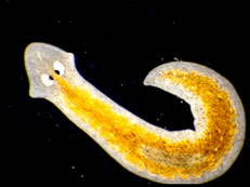 |
||||||||||||||||||||||||||||||||||||||||||||
The hierarchical nature of this design can be appreciated when we examine an illustration of the spatial and temporal scale of the measurements.
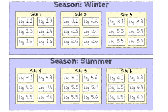
- Within each of the two Seasons, there were three separate Sites (Sites not repeatidly measured across Seasons).
- Within each of the Sites, six logs were selected (haphazardly) from which the number of flatworms were counted.
We construct the model in much the same way. That is:
- The observed number of flatworm per log (for a given Site) is equal to (modelled against) the mean number for that Site
plus a random amount drawn from a normal distribution with a mean of zero and a certain degree of variability (precision).
Number of flatwormlog i = βSite j,i + εi where ε ∼ N(0,σ2)
- The mean number of flatworm per Site (within a given Season) is equal to (modelled against) the mean number for that Season
plus a random amount drawn from a normal distribution with a means of zero and a certain degree of variability (precision).
μSite j = γSeason j + εj where ε ∼ N(0,σ2)
The SITE variable is conveniently already coded as a numeric series (starting at 1).
Open the curdies data file.curdies <- read.table('../downloads/data/curdies.csv', header=T, sep=',', strip.white=T) head(curdies)
  SEASON SITE   DUGESIA   S4DUGES
1 WINTER    1 0.6476829 0.8970995
2 WINTER    1 6.0961516 1.5713175
3 WINTER    1 1.3105639 1.0699526
4 WINTER    1 1.7252788 1.1460797
5 WINTER    1 1.4593867 1.0991136
6 WINTER    1 1.0575610 1.0140897
- Lets start by performing some exploratory data analysis to help us identify any issues with the data as
well as helping to try to identify a possible model to fit.
- Boxplots for the main effect (Season)
Show codeIs there any evidence of non-normality and/or heterogeneity (Y or N)
library(dplyr)
curdies.ag <- curdies %>% group_by(SEASON,SITE) %>% summarize(DUGESIA=mean(DUGESIA))
curdies.ag
Source: local data frame [6 x 3]
Groups: SEASON

  SEASON SITE   DUGESIA
1 SUMMER    4 0.4190947
2 SUMMER    5 0.2290862
3 SUMMER    6 0.1942443
4 WINTER    1 2.0494375
5 WINTER    2 4.1819078
6 WINTER    3 0.6782063
#OR equivalently with the plyr package
library(plyr)
ddply(curdies, ~SEASON+SITE, numcolwise(mean))
  SEASON SITE   DUGESIA   S4DUGES
1 SUMMER    4 0.4190947 0.3508213
2 SUMMER    5 0.2290862 0.1804622
3 SUMMER    6 0.1942443 0.3811223
4 WINTER    1 2.0494375 1.1329421
5 WINTER    2 4.1819078 1.2718698
6 WINTER    3 0.6782063 0.8678707
detach(package:plyr) #since dplyr and plyr do not play nicely together

library(ggplot2)
ggplot(curdies.ag, aes(y=DUGESIA, x=SEASON)) + geom_boxplot()

If so, assess whether a transformation (such as a forth-root transformation) will address the violations and then make the appropriate corrections - Consider a transformation (such as forth-root transform) and redo boxplots for the main effect (Season)
Show codeDoes a forth-root transformation improve the data with respect to normality and homogeneity of variance (Y or N)?
curdies.ag <- curdies %>% group_by(SEASON,SITE) %>% summarize(DUGESIA=mean(DUGESIA^0.25))
curdies.ag
Source: local data frame [6 x 3]
Groups: SEASON

  SEASON SITE   DUGESIA
1 SUMMER    4 0.3508213
2 SUMMER    5 0.1804622
3 SUMMER    6 0.3811223
4 WINTER    1 1.1329421
5 WINTER    2 1.2718698
6 WINTER    3 0.8678707
ggplot(curdies.ag, aes(y=DUGESIA, x=SEASON)) + geom_boxplot()

- Boxplots for the main effect (Season)
- Fit the hierarchical model.
Use with effects (or matrix) parameterization for the 'fixed effects' and means (or matrix) parameterization for the 'random effects'.
Note the following points:
- Non-informative priors for residual precision (standard deviations) should be defined as vague uniform distributions rather than gamma distributions. This prevents the chains from walking to close to parameter estimates of 0. Alternatively, Gelman recommends the use of weakly informative half-cauchy distributions for variances in hierarchical designs.
- Finite-population standard deviation for Site (the within group factor) should reflect standard deviation between Sites within season (not standard deviation between all Sites). Unfortunately, the BUGS language does not offer a mechanism to determine which indexes match certain criteria (for example which Sites correspond to which Season), nor does it allow variables to be redefined. One way to allow us to generate multiple standard deviations is to create an offset vector that can be used to indicate the range of Site numbers that are within which Season.
- As this is a multi-level design in which the Season 'replicates' are determined by the Site means, it is important that firstly, the number of levels of the within Group factor (Season) reflects this, and secondly that the factor levels of the within group factor (Season) correspond to the factor levels of the group factor (Site). In this case, the Sites are labeled 1-6, but the first three Sites are in Winter. R will naturally label Winter as the second level (as alphabetically W comes after S for summer). Thus without intervention or careful awareness, it will appear that the Winter means are higher than the Summer means, when it is actually the other way around. One way to check this, is create the data list and check that all the factor levels are listed in increasing numerical order.
View preparation codesites<-ddply(curdies, ~SITE, catcolwise(unique)) offset <- c(match(levels(sites$SEASON),sites$SEASON), length(sites$SEASON)+1) offset
[1] 4 1 7
curdies.list <- with(curdies,
   list(dugesia=DUGESIA,
        season=as.numeric(SEASON),
                site=as.numeric(SITE),
                n=nrow(curdies), nSeason=length(levels(as.factor(SEASON))),
                nSite=length(levels(as.factor(SITE))),
                SiteOffset=offset
                )
)
curdies.list
$dugesia
 [1]  0.6477  6.0962  1.3106  1.7253  1.4594  1.0576  1.0163 16.1968  1.1681  1.0243  2.0113  3.6746
[13]  0.6891  1.2191  1.1131  0.6569  0.1361  0.2547  0.0000  0.0000  0.9411  0.0000  0.0000  1.5735
[25]  1.3745  0.0000  0.0000  0.0000  0.0000  0.0000  0.0000  0.0000  0.1329  0.0000  0.6580  0.3745

$season
 [1] 2 2 2 2 2 2 2 2 2 2 2 2 2 2 2 2 2 2 1 1 1 1 1 1 1 1 1 1 1 1 1 1 1 1 1 1

$site
 [1] 1 1 1 1 1 1 2 2 2 2 2 2 3 3 3 3 3 3 4 4 4 4 4 4 5 5 5 5 5 5 6 6 6 6 6 6

$n
[1] 36

$nSeason
[1] 2

$nSite
[1] 6

$SiteOffset
[1] 4 1 7
## notice that The Season variable has as many entries as there were plots
## rather than having as many as there were Sites.
## Also notice that Winter is the second Season according to the factor levels
## Finally notice that the offset values are not in order

#season <- with(curdies,SEASON[match(unique(SITE),SITE)])
#season <- factor(season, levels=unique(season))

curdies$SEASON <- factor(curdies$SEASON, levels=c("WINTER","SUMMER"))
sites<-ddply(curdies, ~SITE, catcolwise(unique))
offset <- c(match(levels(sites$SEASON),sites$SEASON), length(sites$SEASON)+1)
offset
[1] 1 4 7
curdies.list <- with(curdies,
   list(dugesia=DUGESIA,
   season=as.numeric(SEASON),
   site=as.numeric(SITE),
   n=nrow(curdies), nSeason=length(levels(SEASON)),
   nSite=length(levels(as.factor(SITE))),
   SiteOffset=offset
   )
)
curdies.list
$dugesia
 [1]  0.6477  6.0962  1.3106  1.7253  1.4594  1.0576  1.0163 16.1968  1.1681  1.0243  2.0113  3.6746
[13]  0.6891  1.2191  1.1131  0.6569  0.1361  0.2547  0.0000  0.0000  0.9411  0.0000  0.0000  1.5735
[25]  1.3745  0.0000  0.0000  0.0000  0.0000  0.0000  0.0000  0.0000  0.1329  0.0000  0.6580  0.3745

$season
 [1] 1 1 1 1 1 1 1 1 1 1 1 1 1 1 1 1 1 1 2 2 2 2 2 2 2 2 2 2 2 2 2 2 2 2 2 2

$site
 [1] 1 1 1 1 1 1 2 2 2 2 2 2 3 3 3 3 3 3 4 4 4 4 4 4 5 5 5 5 5 5 6 6 6 6 6 6

$n
[1] 36

$nSeason
[1] 2

$nSite
[1] 6

$SiteOffset
[1] 1 4 7
## That is betterShow full effects parameterization JAGS codemodelString=" model { #Likelihood for (i in 1:n) { y[i]~dnorm(mu[i],tau) mu[i] <- alpha0 + alpha[SEASON[i]] + beta[SITE[i]] y.err[i] <- y[i] - mu[i] } #Priors alpha0 ~ dnorm(0, 1.0E-6) alpha[1] <- 0 for (i in 2:nSEASON) { alpha[i] ~ dnorm(0, 1.0E-6) #prior } for (i in 1:nSITE) { beta[i] ~ dnorm(0, tau.B) #prior } #Uniform uninformative prior on variance tau <- 1 / (sigma * sigma) tau.B <- 1 / (sigma.B * sigma.B) sigma ~ dunif(0, 100) sigma.B ~ dunif(0, 100) for (i in 1:nSEASON) { SD.Site[i] <- sd(beta[SiteOffset[i]:SiteOffset[i+1]-1]) } sd.Season <- sd(alpha) sd.Site <- mean(SD.Site) #sd(beta.site) sd.Resid <- sd(y.err) } " writeLines(modelString,con="../downloads/BUGSscripts/ws9.2bS1.2a.txt") # Generate a data list curdies$SEASON <- factor(curdies$SEASON, levels=c("WINTER","SUMMER")) sites<-ddply(curdies, ~SITE, catcolwise(unique)) offset <- c(match(levels(sites$SEASON),sites$SEASON), length(sites$SEASON)+1) offset
[1] 1 4 7
curdies$SITE <- factor(curdies$SITE)
curdies.list <- with(curdies,
        list(y=S4DUGES,
         SITE=as.numeric(SITE),
         SEASON=as.numeric(SEASON),
         n=nrow(curdies),
         nSITE=length(levels(SITE)),
         nSEASON = length(levels(SEASON)),
                 SiteOffset=offset
         )
)
curdies.list
$y
 [1] 0.8971 1.5713 1.0700 1.1461 1.0991 1.0141 1.0040 2.0061 1.0396 1.0060 1.1909 1.3845 0.9111 1.0508 1.0272 0.9003 0.6074 0.7104 0.0000 0.0000 0.9849 0.0000 0.0000 1.1200 1.0828 0.0000 0.0000 0.0000
[29] 0.0000 0.0000 0.0000 0.0000 0.6038 0.0000 0.9007 0.7823

$SITE
 [1] 1 1 1 1 1 1 2 2 2 2 2 2 3 3 3 3 3 3 4 4 4 4 4 4 5 5 5 5 5 5 6 6 6 6 6 6

$SEASON
 [1] 1 1 1 1 1 1 1 1 1 1 1 1 1 1 1 1 1 1 2 2 2 2 2 2 2 2 2 2 2 2 2 2 2 2 2 2

$n
[1] 36

$nSITE
[1] 6

$nSEASON
[1] 2

$SiteOffset
[1] 1 4 7
# define parameters
params <- c("alpha0","alpha","sigma","sigma.B","sd.Season","sd.Site","sd.Resid","SD.Site")
burnInSteps = 3000
nChains = 3
numSavedSteps = 3000
thinSteps = 10
nIter = burnInSteps+ceiling((numSavedSteps * thinSteps)/nChains)

library(R2jags)
curdies.r2jags.a <- jags(data=curdies.list,
          inits=NULL,
          parameters.to.save=params,
          model.file="../downloads/BUGSscripts/ws9.2bS1.2a.txt",
          n.chains=nChains,
          n.iter=nIter,
          n.burnin=burnInSteps,
          n.thin=thinSteps
          )
Compiling model graph
   Resolving undeclared variables
   Allocating nodes
   Graph Size: 176

Initializing model
print(curdies.r2jags.a)
Inference for Bugs model at "../downloads/BUGSscripts/ws9.2bS1.2a.txt", fit using jags,
 3 chains, each with 13000 iterations (first 3000 discarded), n.thin = 10
 n.sims = 3000 iterations saved
           mu.vect sd.vect   2.5%    25%    50%    75%  97.5%  Rhat n.eff
SD.Site[1]   0.116   0.091  0.003  0.042  0.098  0.172  0.331 1.006  1300
SD.Site[2]   0.095   0.073  0.003  0.038  0.079  0.135  0.273 1.007   770
alpha[1]     0.000   0.000  0.000  0.000  0.000  0.000  0.000 1.000     1
alpha[2]    -0.789   0.239 -1.261 -0.911 -0.788 -0.662 -0.338 1.002  2100
alpha0       1.093   0.169  0.770  1.010  1.090  1.175  1.426 1.001  2300
sd.Resid     0.387   0.015  0.366  0.377  0.386  0.394  0.425 1.002  3000
sd.Season    0.560   0.160  0.247  0.468  0.557  0.645  0.892 1.005  1200
sd.Site      0.105   0.071  0.004  0.048  0.098  0.151  0.269 1.008   870
sigma        0.404   0.055  0.316  0.366  0.399  0.433  0.529 1.001  3000
sigma.B      0.173   0.164  0.005  0.066  0.128  0.229  0.614 1.008   560
deviance    35.022   3.511 29.717 32.605 34.482 36.802 43.431 1.001  3000

For each parameter, n.eff is a crude measure of effective sample size,
and Rhat is the potential scale reduction factor (at convergence, Rhat=1).

DIC info (using the rule, pD = var(deviance)/2)
pD = 6.2 and DIC = 41.2
DIC is an estimate of expected predictive error (lower deviance is better).
curdies.mcmc.a <- as.mcmc(curdies.r2jags.a)
Show matrix parameterization JAGS codemodelString=" model { #Likelihood for (i in 1:n) { y[i]~dnorm(mu[i],tau) mu[i] <- inprod(alpha[],X[i,]) + beta[SITE[i]] y.err[i] <- y[i] - mu[i] } #Priors alpha ~ dmnorm(a0, A0) for (i in 1:nSITE) { beta[i] ~ dnorm(0, tau.B) #prior } #Uniform uninformative prior on variance tau <- 1 / (sigma * sigma) tau.B <- 1 / (sigma.B * sigma.B) sigma ~ dunif(0, 100) sigma.B ~ dunif(0, 100) # Finite-population standard deviations for (i in 1:nSEASON) { SD.Site[i] <- sd(beta[SiteOffset[i]:SiteOffset[i+1]-1]) } seasons[1] <- alpha[1] for (i in 2:nSEASON) { seasons[i] <- alpha[1]+alpha[i] } sd.Season <- sd(seasons) sd.Site <- mean(SD.Site) sd.Resid <- sd(y.err) } " writeLines(modelString,con="../downloads/BUGSscripts/ws9.2bS1.2b.txt") # Generate a data list curdies$SEASON <- factor(curdies$SEASON, levels=c("WINTER","SUMMER")) sites<-ddply(curdies, ~SITE, catcolwise(unique)) offset <- c(match(levels(sites$SEASON),sites$SEASON), length(sites$SEASON)+1) offset
[1] 1 4 7
curdies$SITE <- factor(curdies$SITE)
Xmat <- model.matrix(~SEASON, data=curdies)
curdies.list <- with(curdies,
        list(y=S4DUGES,
         SITE=as.numeric(SITE),
         X=Xmat,
         n=nrow(curdies),
         nSITE=length(levels(SITE)),
                 nSEASON=length(levels(SEASON)),
         a0=rep(0, ncol(Xmat)), A0=diag(0, ncol(Xmat)),
                 SiteOffset=offset
         )
)
curdies.list
$y
 [1] 0.8971 1.5713 1.0700 1.1461 1.0991 1.0141 1.0040 2.0061 1.0396 1.0060 1.1909 1.3845 0.9111 1.0508 1.0272 0.9003 0.6074 0.7104 0.0000 0.0000 0.9849 0.0000 0.0000 1.1200 1.0828 0.0000 0.0000 0.0000
[29] 0.0000 0.0000 0.0000 0.0000 0.6038 0.0000 0.9007 0.7823

$SITE
 [1] 1 1 1 1 1 1 2 2 2 2 2 2 3 3 3 3 3 3 4 4 4 4 4 4 5 5 5 5 5 5 6 6 6 6 6 6

$X
   (Intercept) SEASONSUMMER
1            1            0
2            1            0
3            1            0
4            1            0
5            1            0
6            1            0
7            1            0
8            1            0
9            1            0
10           1            0
11           1            0
12           1            0
13           1            0
14           1            0
15           1            0
16           1            0
17           1            0
18           1            0
19           1            1
20           1            1
21           1            1
22           1            1
23           1            1
24           1            1
25           1            1
26           1            1
27           1            1
28           1            1
29           1            1
30           1            1
31           1            1
32           1            1
33           1            1
34           1            1
35           1            1
36           1            1
attr(,"assign")
[1] 0 1
attr(,"contrasts")
attr(,"contrasts")$SEASON
[1] "contr.treatment"


$n
[1] 36

$nSITE
[1] 6

$nSEASON
[1] 2

$a0
[1] 0 0

$A0
     [,1] [,2]
[1,]    0    0
[2,]    0    0

$SiteOffset
[1] 1 4 7
# define parameters params <- c("alpha","sigma","sigma.B","sd.Season","sd.Site","sd.Resid","SD.Site") burnInSteps = 3000 nChains = 3 numSavedSteps = 3000 thinSteps = 10 nIter = burnInSteps+ceiling((numSavedSteps * thinSteps)/nChains) library(R2jags) curdies.r2jags.b <- jags(data=curdies.list, inits=NULL, parameters.to.save=params, model.file="../downloads/BUGSscripts/ws9.2bS1.2b.txt", n.chains=nChains, n.iter=nIter, n.burnin=burnInSteps, n.thin=thinSteps )
Compiling model graph
   Resolving undeclared variables
   Allocating nodes
   Graph Size: 258

Initializing model
print(curdies.r2jags.b)
Inference for Bugs model at "../downloads/BUGSscripts/ws9.2bS1.2b.txt", fit using jags,
 3 chains, each with 13000 iterations (first 3000 discarded), n.thin = 10
 n.sims = 3000 iterations saved
           mu.vect sd.vect   2.5%    25%    50%    75%  97.5%  Rhat n.eff
SD.Site[1]   0.115   0.090  0.004  0.041  0.096  0.171  0.324 1.015   490
SD.Site[2]   0.092   0.071  0.003  0.036  0.077  0.134  0.265 1.023   370
alpha[1]     1.088   0.170  0.756  1.001  1.085  1.176  1.425 1.005  2400
alpha[2]    -0.786   0.230 -1.245 -0.907 -0.786 -0.663 -0.327 1.002  3000
sd.Resid     0.388   0.015  0.366  0.378  0.386  0.394  0.424 1.001  3000
sd.Season    0.557   0.158  0.237  0.469  0.556  0.642  0.880 1.001  3000
sd.Site      0.104   0.070  0.004  0.046  0.094  0.151  0.258 1.028   330
sigma        0.403   0.054  0.315  0.366  0.396  0.434  0.522 1.001  3000
sigma.B      0.169   0.157  0.006  0.064  0.132  0.226  0.552 1.022   440
deviance    35.038   3.445 29.819 32.678 34.494 36.737 43.569 1.001  3000

For each parameter, n.eff is a crude measure of effective sample size,
and Rhat is the potential scale reduction factor (at convergence, Rhat=1).

DIC info (using the rule, pD = var(deviance)/2)
pD = 5.9 and DIC = 41.0
DIC is an estimate of expected predictive error (lower deviance is better).
curdies.mcmc.b <- as.mcmc(curdies.r2jags.b)
Hierarchical parameterization JAGS codemodelString=" model { #Likelihood #Likelihood (esimating site means (gamma.site) for (i in 1:n) { y[i]~dnorm(quad.means[i],tau) quad.means[i] <- gamma.site[SITE[i]] y.err[i] <- y[i] - quad.means[i] } for (i in 1:nSITE) { gamma.site[i] ~ dnorm(site.means[i], tau.site) site.means[i] <- inprod(beta[],X[i,]) } #Priors for (i in 1:nX) { beta[i] ~ dnorm(0, 1.0E-6) #prior } sigma ~ dunif(0, 100) tau <- 1 / (sigma * sigma) sigma.site ~ dunif(0, 100) tau.site <- 1 / (sigma.site * sigma.site) # Finite-population standard deviations for (i in 1:nSEASON) { SD.Site[i] <- sd(gamma.site[SiteOffset[i]:SiteOffset[i+1]-1]) } seasons[1] <- beta[1] for (i in 2:nSEASON) { seasons[i] <- beta[1]+beta[i] } sd.Season <- sd(seasons) sd.Site <- mean(SD.Site) sd.Resid <- sd(y.err) } " writeLines(modelString,con="../downloads/BUGSscripts/ws9.2bS1.2c.txt") # Generate a data list curdies$SEASON <- factor(curdies$SEASON, levels=c("WINTER","SUMMER")) sites<-ddply(curdies, ~SITE, catcolwise(unique)) offset <- c(match(levels(sites$SEASON),sites$SEASON), length(sites$SEASON)+1) offset
[1] 1 4 7
curdies$SITE <- factor(curdies$SITE)
Xmat <- model.matrix(~SEASON, data=ddply(curdies, ~SITE, catcolwise(unique)))
curdies.list <- with(curdies,
        list(y=S4DUGES,
         SITE=as.numeric(SITE),
         X=Xmat,
         nX=ncol(Xmat),
         n=nrow(curdies),
         nSITE=length(levels(SITE)),
                 nSEASON=length(levels(SEASON)),
                 SiteOffset=offset
         )
)
curdies.list
$y
 [1] 0.8971 1.5713 1.0700 1.1461 1.0991 1.0141 1.0040 2.0061 1.0396 1.0060 1.1909 1.3845 0.9111 1.0508 1.0272 0.9003 0.6074 0.7104 0.0000 0.0000 0.9849 0.0000 0.0000 1.1200 1.0828 0.0000 0.0000 0.0000
[29] 0.0000 0.0000 0.0000 0.0000 0.6038 0.0000 0.9007 0.7823

$SITE
 [1] 1 1 1 1 1 1 2 2 2 2 2 2 3 3 3 3 3 3 4 4 4 4 4 4 5 5 5 5 5 5 6 6 6 6 6 6

$X
  (Intercept) SEASONSUMMER
1           1            0
2           1            0
3           1            0
4           1            1
5           1            1
6           1            1
attr(,"assign")
[1] 0 1
attr(,"contrasts")
attr(,"contrasts")$SEASON
[1] "contr.treatment"


$nX
[1] 2

$n
[1] 36

$nSITE
[1] 6

$nSEASON
[1] 2

$SiteOffset
[1] 1 4 7
# define parameters
params <- c("beta","sigma","sigma.site","sd.Season","sd.Site","sd.Resid")
burnInSteps = 3000
nChains = 3
numSavedSteps = 3000
thinSteps = 10
nIter = burnInSteps+ceiling((numSavedSteps * thinSteps)/nChains)

library(R2jags)
curdies.r2jags.c <- jags(data=curdies.list,
          inits=NULL,
          parameters.to.save=params,
          model.file="../downloads/BUGSscripts/ws9.2bS1.2c.txt",
          n.chains=nChains,
          n.iter=nIter,
          n.burnin=burnInSteps,
          n.thin=thinSteps
          )
Compiling model graph
   Resolving undeclared variables
   Allocating nodes
   Graph Size: 156

Initializing model
print(curdies.r2jags.c)
Inference for Bugs model at "../downloads/BUGSscripts/ws9.2bS1.2c.txt", fit using jags,
 3 chains, each with 13000 iterations (first 3000 discarded), n.thin = 10
 n.sims = 3000 iterations saved
           mu.vect sd.vect   2.5%    25%    50%    75%  97.5%  Rhat n.eff
beta[1]      1.089   0.172  0.757  1.001  1.086  1.178  1.414 1.001  3000
beta[2]     -0.783   0.241 -1.255 -0.905 -0.780 -0.662 -0.350 1.001  3000
sd.Resid     0.388   0.015  0.366  0.377  0.386  0.394  0.423 1.002  1800
sd.Season    0.556   0.162  0.254  0.468  0.552  0.640  0.887 1.006  3000
sd.Site      0.104   0.071  0.003  0.047  0.094  0.150  0.261 1.003   970
sigma        0.402   0.053  0.314  0.365  0.396  0.433  0.515 1.002  1400
sigma.site   0.179   0.187  0.004  0.061  0.134  0.235  0.654 1.002  1100
deviance    34.970   3.365 29.820 32.577 34.405 36.866 42.802 1.001  3000

For each parameter, n.eff is a crude measure of effective sample size,
and Rhat is the potential scale reduction factor (at convergence, Rhat=1).

DIC info (using the rule, pD = var(deviance)/2)
pD = 5.7 and DIC = 40.6
DIC is an estimate of expected predictive error (lower deviance is better).
curdies.mcmc.c <- as.mcmc(curdies.r2jags.c)
Matrix parameterization STAN codeUnfortunately, STAN does not yet support vector indexing or the ability to multiply a matrix by a vector. A work around involves multiplication of a dummy matrix with the gamma vector..rstanString= # Generate a data list curdies$SEASON <- factor(curdies$SEASON, levels=c("WINTER","SUMMER")) sites<-ddply(curdies, ~SITE, catcolwise(unique)) offset <- c(match(levels(sites$SEASON),sites$SEASON), length(sites$SEASON)+1) offset
[1] 1 4 7
curdies$SITE <- factor(curdies$SITE)
Xmat <- model.matrix(~SEASON, data=curdies)
Zmat <- model.matrix(~-1+SITE, data=curdies)
curdies.list <- with(curdies,
        list(y=S4DUGES,
         Z=Zmat,
         X=Xmat,
         nX=ncol(Xmat),
                 nZ=ncol(Zmat),
         n=nrow(curdies),
         a0=rep(0,ncol(Xmat)), A0=diag(100000,ncol(Xmat)),
         SiteOffset=offset,
         m=matrix(rep(1,6),2)
         )
)
curdies.list
$y
 [1] 0.8971 1.5713 1.0700 1.1461 1.0991 1.0141 1.0040 2.0061 1.0396 1.0060 1.1909 1.3845 0.9111 1.0508 1.0272 0.9003 0.6074 0.7104 0.0000 0.0000 0.9849 0.0000 0.0000 1.1200 1.0828 0.0000 0.0000 0.0000
[29] 0.0000 0.0000 0.0000 0.0000 0.6038 0.0000 0.9007 0.7823

$Z
   SITE1 SITE2 SITE3 SITE4 SITE5 SITE6
1      1     0     0     0     0     0
2      1     0     0     0     0     0
3      1     0     0     0     0     0
4      1     0     0     0     0     0
5      1     0     0     0     0     0
6      1     0     0     0     0     0
7      0     1     0     0     0     0
8      0     1     0     0     0     0
9      0     1     0     0     0     0
10     0     1     0     0     0     0
11     0     1     0     0     0     0
12     0     1     0     0     0     0
13     0     0     1     0     0     0
14     0     0     1     0     0     0
15     0     0     1     0     0     0
16     0     0     1     0     0     0
17     0     0     1     0     0     0
18     0     0     1     0     0     0
19     0     0     0     1     0     0
20     0     0     0     1     0     0
21     0     0     0     1     0     0
22     0     0     0     1     0     0
23     0     0     0     1     0     0
24     0     0     0     1     0     0
25     0     0     0     0     1     0
26     0     0     0     0     1     0
27     0     0     0     0     1     0
28     0     0     0     0     1     0
29     0     0     0     0     1     0
30     0     0     0     0     1     0
31     0     0     0     0     0     1
32     0     0     0     0     0     1
33     0     0     0     0     0     1
34     0     0     0     0     0     1
35     0     0     0     0     0     1
36     0     0     0     0     0     1
attr(,"assign")
[1] 1 1 1 1 1 1
attr(,"contrasts")
attr(,"contrasts")$SITE
[1] "contr.treatment"


$X
   (Intercept) SEASONSUMMER
1            1            0
2            1            0
3            1            0
4            1            0
5            1            0
6            1            0
7            1            0
8            1            0
9            1            0
10           1            0
11           1            0
12           1            0
13           1            0
14           1            0
15           1            0
16           1            0
17           1            0
18           1            0
19           1            1
20           1            1
21           1            1
22           1            1
23           1            1
24           1            1
25           1            1
26           1            1
27           1            1
28           1            1
29           1            1
30           1            1
31           1            1
32           1            1
33           1            1
34           1            1
35           1            1
36           1            1
attr(,"assign")
[1] 0 1
attr(,"contrasts")
attr(,"contrasts")$SEASON
[1] "contr.treatment"


$nX
[1] 2

$nZ
[1] 6

$n
[1] 36

$a0
[1] 0 0

$A0
      [,1]  [,2]
[1,] 1e+05 0e+00
[2,] 0e+00 1e+05

$SiteOffset
[1] 1 4 7

$m
     [,1] [,2] [,3]
[1,]    1    1    1
[2,]    1    1    1
# define parameters burnInSteps = 3000 nChains = 3 numSavedSteps = 3000 thinSteps = 10 nIter = burnInSteps+ceiling((numSavedSteps * thinSteps)/nChains) library(rstan) curdies.rstan.a <- stan(data=curdies.list, model_code=rstanString, pars=c('beta','gamma','sigma','sigma_Z','sd_Resid','sd_Season','sd_Site'), chains=nChains, iter=nIter, warmup=burnInSteps, thin=thinSteps, save_dso=TRUE )
TRANSLATING MODEL 'rstanString' FROM Stan CODE TO C++ CODE NOW.
COMPILING THE C++ CODE FOR MODEL 'rstanString' NOW.

SAMPLING FOR MODEL 'rstanString' NOW (CHAIN 1).

Iteration:     1 / 13000 [  0%]  (Warmup)
Iteration:  1300 / 13000 [ 10%]  (Warmup)
Iteration:  2600 / 13000 [ 20%]  (Warmup)
Iteration:  3001 / 13000 [ 23%]  (Sampling)
Iteration:  4300 / 13000 [ 33%]  (Sampling)
Iteration:  5600 / 13000 [ 43%]  (Sampling)
Iteration:  6900 / 13000 [ 53%]  (Sampling)
Iteration:  8200 / 13000 [ 63%]  (Sampling)
Iteration:  9500 / 13000 [ 73%]  (Sampling)
Iteration: 10800 / 13000 [ 83%]  (Sampling)
Iteration: 12100 / 13000 [ 93%]  (Sampling)
Iteration: 13000 / 13000 [100%]  (Sampling)
#  Elapsed Time: 0.42 seconds (Warm-up)
#                1.39 seconds (Sampling)
#                1.81 seconds (Total)


SAMPLING FOR MODEL 'rstanString' NOW (CHAIN 2).

Iteration:     1 / 13000 [  0%]  (Warmup)
Iteration:  1300 / 13000 [ 10%]  (Warmup)
Iteration:  2600 / 13000 [ 20%]  (Warmup)
Iteration:  3001 / 13000 [ 23%]  (Sampling)
Iteration:  4300 / 13000 [ 33%]  (Sampling)
Iteration:  5600 / 13000 [ 43%]  (Sampling)
Iteration:  6900 / 13000 [ 53%]  (Sampling)
Iteration:  8200 / 13000 [ 63%]  (Sampling)
Iteration:  9500 / 13000 [ 73%]  (Sampling)
Iteration: 10800 / 13000 [ 83%]  (Sampling)
Iteration: 12100 / 13000 [ 93%]  (Sampling)
Iteration: 13000 / 13000 [100%]  (Sampling)
#  Elapsed Time: 0.45 seconds (Warm-up)
#                1.56 seconds (Sampling)
#                2.01 seconds (Total)


SAMPLING FOR MODEL 'rstanString' NOW (CHAIN 3).

Iteration:     1 / 13000 [  0%]  (Warmup)
Iteration:  1300 / 13000 [ 10%]  (Warmup)
Iteration:  2600 / 13000 [ 20%]  (Warmup)
Iteration:  3001 / 13000 [ 23%]  (Sampling)
Iteration:  4300 / 13000 [ 33%]  (Sampling)
Iteration:  5600 / 13000 [ 43%]  (Sampling)
Iteration:  6900 / 13000 [ 53%]  (Sampling)
Iteration:  8200 / 13000 [ 63%]  (Sampling)
Iteration:  9500 / 13000 [ 73%]  (Sampling)
Iteration: 10800 / 13000 [ 83%]  (Sampling)
Iteration: 12100 / 13000 [ 93%]  (Sampling)
Iteration: 13000 / 13000 [100%]  (Sampling)
#  Elapsed Time: 0.41 seconds (Warm-up)
#                1.42 seconds (Sampling)
#                1.83 seconds (Total)
print(curdies.rstan.a)
Inference for Stan model: rstanString.
3 chains, each with iter=13000; warmup=3000; thin=10;
post-warmup draws per chain=1000, total post-warmup draws=3000.

           mean se_mean   sd  2.5%   25%   50%   75% 97.5% n_eff Rhat
beta[1]    1.09    0.00 0.18  0.72  0.99  1.09  1.18  1.42  3000    1
beta[2]   -0.78    0.01 0.24 -1.22 -0.91 -0.78 -0.65 -0.30  2248    1
gamma[1]   0.03    0.00 0.17 -0.30 -0.05  0.01  0.09  0.42  3000    1
gamma[2]   0.08    0.00 0.18 -0.22 -0.01  0.04  0.15  0.51  2431    1
gamma[3]  -0.09    0.00 0.19 -0.53 -0.17 -0.06  0.00  0.19  2813    1
gamma[4]   0.02    0.00 0.17 -0.33 -0.05  0.01  0.09  0.36  3000    1
gamma[5]  -0.06    0.00 0.17 -0.46 -0.12 -0.03  0.02  0.23  2882    1
gamma[6]   0.03    0.00 0.17 -0.29 -0.04  0.02  0.10  0.40  2857    1
sigma      0.40    0.00 0.05  0.32  0.37  0.40  0.44  0.53  1447    1
sigma_Z    0.19    0.00 0.18  0.02  0.07  0.14  0.24  0.62  1463    1
sd_Resid   0.39    0.00 0.02  0.37  0.38  0.39  0.39  0.42  2299    1
sd_Season  0.55    0.00 0.16  0.22  0.46  0.55  0.64  0.87  2129    1
sd_Site    0.11    0.00 0.07  0.01  0.06  0.10  0.16  0.26   874    1
lp__      22.43    0.20 4.50 13.77 19.47 22.24 25.20 31.53   518    1

Samples were drawn using NUTS(diag_e) at Sun Mar  8 15:28:34 2015.
For each parameter, n_eff is a crude measure of effective sample size,
and Rhat is the potential scale reduction factor on split chains (at
convergence, Rhat=1).
curdies.mcmc.d <- rstan:::as.mcmc.list.stanfit(curdies.rstan.a) curdies.mcmc.df.d <- as.data.frame(extract(curdies.rstan.a)) SD.site <- NULL sd.site <- curdies.mcmc.df.d[,3:8] for (i in 1:length(levels(curdies$SEASON))) { SD.site <- c(SD.site,apply(sd.site[,offset[i]:(offset[i+1]-1)],1,sd)) } data.frame(mean=mean(SD.site), median=median(SD.site), HPDinterval(as.mcmc(SD.site)), HPDinterval(as.mcmc(SD.site),p=0.68))
       mean  median    lower  upper  lower.1 upper.1
var1 0.1115 0.09236 0.003046 0.2739 0.003046  0.1377
Hierarchical parameterization STAN coderstanString=" data{ int n; int nZ; int nX; vector [n] y; matrix [nZ,nX] X; matrix [n,nZ] Z; } parameters{ vector [nX] beta; real<lower=0> sigma; vector [nZ] gamma; real<lower=0> sigma_Z; } transformed parameters { vector [n] mu_Z; vector [nZ] mu; mu_Z <- Z*gamma; mu <- X*beta; } model{ // Priors beta ~ normal(0, 10000); gamma ~ normal( 0 , 1000); sigma_Z ~ uniform( 0 , 100 ); sigma ~ uniform( 0 , 100 ); y ~ normal(mu_Z, sigma); gamma ~ normal( mu , sigma_Z ); } generated quantities { vector [n] y_err; real<lower=0> sd_Resid; y_err <- y - mu_Z; sd_Resid <- sd(y_err); } " # Generate a data list curdies$SITE <- factor(curdies$SITE) Xmat <- model.matrix(~SEASON, data=ddply(curdies, ~SITE, catcolwise(unique))) Zmat <- model.matrix(~-1+SITE, data=curdies) curdies.list <- with(curdies, list(y=S4DUGES, Z=Zmat, X=Xmat, nX=ncol(Xmat), nZ=ncol(Zmat), n=nrow(curdies) ) ) curdies.list
$y
 [1] 0.8971 1.5713 1.0700 1.1461 1.0991 1.0141 1.0040 2.0061 1.0396 1.0060 1.1909 1.3845 0.9111 1.0508 1.0272 0.9003 0.6074 0.7104 0.0000 0.0000 0.9849 0.0000 0.0000 1.1200 1.0828 0.0000 0.0000 0.0000
[29] 0.0000 0.0000 0.0000 0.0000 0.6038 0.0000 0.9007 0.7823

$Z
   SITE1 SITE2 SITE3 SITE4 SITE5 SITE6
1      1     0     0     0     0     0
2      1     0     0     0     0     0
3      1     0     0     0     0     0
4      1     0     0     0     0     0
5      1     0     0     0     0     0
6      1     0     0     0     0     0
7      0     1     0     0     0     0
8      0     1     0     0     0     0
9      0     1     0     0     0     0
10     0     1     0     0     0     0
11     0     1     0     0     0     0
12     0     1     0     0     0     0
13     0     0     1     0     0     0
14     0     0     1     0     0     0
15     0     0     1     0     0     0
16     0     0     1     0     0     0
17     0     0     1     0     0     0
18     0     0     1     0     0     0
19     0     0     0     1     0     0
20     0     0     0     1     0     0
21     0     0     0     1     0     0
22     0     0     0     1     0     0
23     0     0     0     1     0     0
24     0     0     0     1     0     0
25     0     0     0     0     1     0
26     0     0     0     0     1     0
27     0     0     0     0     1     0
28     0     0     0     0     1     0
29     0     0     0     0     1     0
30     0     0     0     0     1     0
31     0     0     0     0     0     1
32     0     0     0     0     0     1
33     0     0     0     0     0     1
34     0     0     0     0     0     1
35     0     0     0     0     0     1
36     0     0     0     0     0     1
attr(,"assign")
[1] 1 1 1 1 1 1
attr(,"contrasts")
attr(,"contrasts")$SITE
[1] "contr.treatment"


$X
  (Intercept) SEASONSUMMER
1           1            0
2           1            0
3           1            0
4           1            1
5           1            1
6           1            1
attr(,"assign")
[1] 0 1
attr(,"contrasts")
attr(,"contrasts")$SEASON
[1] "contr.treatment"


$nX
[1] 2

$nZ
[1] 6

$n
[1] 36
# define parameters
burnInSteps = 3000
nChains = 3
numSavedSteps = 3000
thinSteps = 10
nIter = burnInSteps+ceiling((numSavedSteps * thinSteps)/nChains)

library(rstan)
curdies.rstan.b <- stan(data=curdies.list,
      model_code=rstanString,
          pars=c('beta','gamma','sigma','sigma_Z','sd_Resid'),
          chains=nChains,
          iter=nIter,
          warmup=burnInSteps,
          thin=thinSteps,
      save_dso=TRUE
          )
TRANSLATING MODEL 'rstanString' FROM Stan CODE TO C++ CODE NOW.
COMPILING THE C++ CODE FOR MODEL 'rstanString' NOW.

SAMPLING FOR MODEL 'rstanString' NOW (CHAIN 1).

Iteration:     1 / 13000 [  0%]  (Warmup)
Iteration:  1300 / 13000 [ 10%]  (Warmup)
Iteration:  2600 / 13000 [ 20%]  (Warmup)
Iteration:  3001 / 13000 [ 23%]  (Sampling)
Iteration:  4300 / 13000 [ 33%]  (Sampling)
Iteration:  5600 / 13000 [ 43%]  (Sampling)
Iteration:  6900 / 13000 [ 53%]  (Sampling)
Iteration:  8200 / 13000 [ 63%]  (Sampling)
Iteration:  9500 / 13000 [ 73%]  (Sampling)
Iteration: 10800 / 13000 [ 83%]  (Sampling)
Iteration: 12100 / 13000 [ 93%]  (Sampling)
Iteration: 13000 / 13000 [100%]  (Sampling)
#  Elapsed Time: 0.48 seconds (Warm-up)
#                2.24 seconds (Sampling)
#                2.72 seconds (Total)


SAMPLING FOR MODEL 'rstanString' NOW (CHAIN 2).

Iteration:     1 / 13000 [  0%]  (Warmup)
Iteration:  1300 / 13000 [ 10%]  (Warmup)
Iteration:  2600 / 13000 [ 20%]  (Warmup)
Iteration:  3001 / 13000 [ 23%]  (Sampling)
Iteration:  4300 / 13000 [ 33%]  (Sampling)
Iteration:  5600 / 13000 [ 43%]  (Sampling)
Iteration:  6900 / 13000 [ 53%]  (Sampling)
Iteration:  8200 / 13000 [ 63%]  (Sampling)
Iteration:  9500 / 13000 [ 73%]  (Sampling)
Iteration: 10800 / 13000 [ 83%]  (Sampling)
Iteration: 12100 / 13000 [ 93%]  (Sampling)
Iteration: 13000 / 13000 [100%]  (Sampling)
#  Elapsed Time: 0.39 seconds (Warm-up)
#                0.94 seconds (Sampling)
#                1.33 seconds (Total)


SAMPLING FOR MODEL 'rstanString' NOW (CHAIN 3).

Iteration:     1 / 13000 [  0%]  (Warmup)
Iteration:  1300 / 13000 [ 10%]  (Warmup)
Iteration:  2600 / 13000 [ 20%]  (Warmup)
Iteration:  3001 / 13000 [ 23%]  (Sampling)
Iteration:  4300 / 13000 [ 33%]  (Sampling)
Iteration:  5600 / 13000 [ 43%]  (Sampling)
Iteration:  6900 / 13000 [ 53%]  (Sampling)
Iteration:  8200 / 13000 [ 63%]  (Sampling)
Iteration:  9500 / 13000 [ 73%]  (Sampling)
Iteration: 10800 / 13000 [ 83%]  (Sampling)
Iteration: 12100 / 13000 [ 93%]  (Sampling)
Iteration: 13000 / 13000 [100%]  (Sampling)
#  Elapsed Time: 0.44 seconds (Warm-up)
#                0.98 seconds (Sampling)
#                1.42 seconds (Total)
print(curdies.rstan.b)
Inference for Stan model: rstanString.
3 chains, each with iter=13000; warmup=3000; thin=10;
post-warmup draws per chain=1000, total post-warmup draws=3000.

          mean se_mean   sd  2.5%   25%   50%   75% 97.5% n_eff Rhat
beta[1]   1.09    0.00 0.17  0.77  1.00  1.09  1.18  1.44  2750 1.00
beta[2]  -0.78    0.01 0.25 -1.25 -0.91 -0.79 -0.65 -0.26  2189 1.00
gamma[1]  1.11    0.00 0.13  0.85  1.01  1.11  1.19  1.37  1590 1.00
gamma[2]  1.17    0.00 0.14  0.92  1.07  1.16  1.25  1.47  1851 1.00
gamma[3]  0.99    0.00 0.14  0.68  0.91  1.00  1.09  1.26  1739 1.00
gamma[4]  0.33    0.00 0.13  0.08  0.24  0.33  0.42  0.60  1059 1.00
gamma[5]  0.25    0.00 0.13 -0.03  0.17  0.26  0.34  0.50  1228 1.00
gamma[6]  0.34    0.00 0.13  0.09  0.25  0.34  0.43  0.60  1176 1.00
sigma     0.40    0.00 0.05  0.31  0.36  0.39  0.43  0.52  1665 1.00
sigma_Z   0.19    0.01 0.18  0.03  0.07  0.14  0.24  0.64  1065 1.00
sd_Resid  0.39    0.00 0.01  0.37  0.38  0.38  0.39  0.42  2307 1.00
lp__     22.25    0.17 4.10 13.61 19.58 22.37 25.13 29.87   560 1.01

Samples were drawn using NUTS(diag_e) at Sun Mar  8 15:29:07 2015.
For each parameter, n_eff is a crude measure of effective sample size,
and Rhat is the potential scale reduction factor on split chains (at
convergence, Rhat=1).
curdies.mcmc.e <- rstan:::as.mcmc.list.stanfit(curdies.rstan.b) curdies.mcmc.df.e <- as.data.frame(extract(curdies.rstan.b))
#Finite-population standard deviations
## Seasons
seasons <- NULL
seasons <- cbind(curdies.mcmc.df.e[,'beta.1'],
                 curdies.mcmc.df.e[,'beta.1']+curdies.mcmc.df.e[,'beta.2'])
sd.season <- apply(seasons,1,sd)
library(coda)
data.frame(mean=mean(sd.season), median=median(sd.season), HPDinterval(as.mcmc(sd.season)), HPDinterval(as.mcmc(sd.season),p=0.68))
          mean    median     lower     upper   lower.1   upper.1
var1 0.5536985 0.5585557 0.1999721 0.8859165 0.4131178 0.6909496
## Sites
SD.site <- NULL
sd.site <- curdies.mcmc.df.e[,3:8]
for (i in 1:length(levels(curdies$SEASON))) {
  SD.site <-  c(SD.site,apply(sd.site[,offset[i]:(offset[i+1]-1)],1,sd))
}
data.frame(mean=mean(SD.site), median=median(SD.site), HPDinterval(as.mcmc(SD.site)), HPDinterval(as.mcmc(SD.site),p=0.68))
          mean     median       lower     upper    lower.1   upper.1
var1 0.1115323 0.09316411 0.001736477 0.2707392 0.01333439 0.1432832
BRM codecurdies.brm <- brm(S4DUGES ~ SEASON + (1|SITE), data=curdies, family='gaussian', prior=c(set_prior('normal(0,100)', class='b'), set_prior('cauchy(0,5)', class='sd')), n.chains=3, n.iter=2000, warmup=500, n.thin=2 )
SAMPLING FOR MODEL 'gaussian(identity) brms-model' NOW (CHAIN 1).

Chain 1, Iteration:    1 / 2000 [  0%]  (Warmup)
Chain 1, Iteration:  200 / 2000 [ 10%]  (Warmup)
Chain 1, Iteration:  400 / 2000 [ 20%]  (Warmup)
Chain 1, Iteration:  501 / 2000 [ 25%]  (Sampling)
Chain 1, Iteration:  700 / 2000 [ 35%]  (Sampling)
Chain 1, Iteration:  900 / 2000 [ 45%]  (Sampling)
Chain 1, Iteration: 1100 / 2000 [ 55%]  (Sampling)
Chain 1, Iteration: 1300 / 2000 [ 65%]  (Sampling)
Chain 1, Iteration: 1500 / 2000 [ 75%]  (Sampling)
Chain 1, Iteration: 1700 / 2000 [ 85%]  (Sampling)
Chain 1, Iteration: 1900 / 2000 [ 95%]  (Sampling)
Chain 1, Iteration: 2000 / 2000 [100%]  (Sampling)
#  Elapsed Time: 0.108542 seconds (Warm-up)
#                0.196446 seconds (Sampling)
#                0.304988 seconds (Total)


SAMPLING FOR MODEL 'gaussian(identity) brms-model' NOW (CHAIN 2).

Chain 2, Iteration:    1 / 2000 [  0%]  (Warmup)
Chain 2, Iteration:  200 / 2000 [ 10%]  (Warmup)
Chain 2, Iteration:  400 / 2000 [ 20%]  (Warmup)
Chain 2, Iteration:  501 / 2000 [ 25%]  (Sampling)
Chain 2, Iteration:  700 / 2000 [ 35%]  (Sampling)
Chain 2, Iteration:  900 / 2000 [ 45%]  (Sampling)
Chain 2, Iteration: 1100 / 2000 [ 55%]  (Sampling)
Chain 2, Iteration: 1300 / 2000 [ 65%]  (Sampling)
Chain 2, Iteration: 1500 / 2000 [ 75%]  (Sampling)
Chain 2, Iteration: 1700 / 2000 [ 85%]  (Sampling)
Chain 2, Iteration: 1900 / 2000 [ 95%]  (Sampling)
Chain 2, Iteration: 2000 / 2000 [100%]  (Sampling)
#  Elapsed Time: 0.104188 seconds (Warm-up)
#                0.295826 seconds (Sampling)
#                0.400014 seconds (Total)


SAMPLING FOR MODEL 'gaussian(identity) brms-model' NOW (CHAIN 3).

Chain 3, Iteration:    1 / 2000 [  0%]  (Warmup)
Chain 3, Iteration:  200 / 2000 [ 10%]  (Warmup)
Chain 3, Iteration:  400 / 2000 [ 20%]  (Warmup)
Chain 3, Iteration:  501 / 2000 [ 25%]  (Sampling)
Chain 3, Iteration:  700 / 2000 [ 35%]  (Sampling)
Chain 3, Iteration:  900 / 2000 [ 45%]  (Sampling)
Chain 3, Iteration: 1100 / 2000 [ 55%]  (Sampling)
Chain 3, Iteration: 1300 / 2000 [ 65%]  (Sampling)
Chain 3, Iteration: 1500 / 2000 [ 75%]  (Sampling)
Chain 3, Iteration: 1700 / 2000 [ 85%]  (Sampling)
Chain 3, Iteration: 1900 / 2000 [ 95%]  (Sampling)
Chain 3, Iteration: 2000 / 2000 [100%]  (Sampling)
#  Elapsed Time: 0.17552 seconds (Warm-up)
#                0.196082 seconds (Sampling)
#                0.371602 seconds (Total)
summary(curdies.brm)
Family: gaussian (identity) Formula: S4DUGES ~ SEASON + (1 | SITE) Data: curdies (Number of observations: 36) Samples: 3 chains, each with n.iter = 2000; n.warmup = 500; n.thin = 2; total post-warmup samples = 2250 WAIC: 39.88 Random Effects: ~SITE (Number of levels: 6) Estimate Est.Error l-95% CI u-95% CI Eff.Sample Rhat sd(Intercept) 0.18 0.16 0.01 0.62 567 1 Fixed Effects: Estimate Est.Error l-95% CI u-95% CI Eff.Sample Rhat Intercept 1.09 0.17 0.74 1.45 479 1.01 SEASONSUMMER -0.79 0.22 -1.25 -0.34 713 1.00 Family Specific Parameters: Estimate Est.Error l-95% CI u-95% CI Eff.Sample Rhat sigma(S4DUGES) 0.4 0.05 0.31 0.53 1726 1 Samples were drawn using NUTS(diag_e). For each parameter, Eff.Sample is a crude measure of effective sample size, and Rhat is the potential scale reduction factor on split chains (at convergence, Rhat = 1).brms:::stancode(curdies.brm)
functions {
}
data {
  int<lower=1> N;  # number of observations
  vector[N] Y;  # response variable
  int<lower=1> K;  # number of fixed effects
  matrix[N, K] X;  # FE design matrix
  # data for random effects of SITE
  int<lower=1> J_1[N];  # RE levels
  int<lower=1> N_1;  # number of levels
  int<lower=1> K_1;  # number of REs
  real Z_1[N];  # RE design matrix
}
transformed data {
}
parameters {
  real b_Intercept;  # fixed effects Intercept
  vector[K] b;  # fixed effects
  vector[N_1] pre_1;  # unscaled REs
  real<lower=0> sd_1;  # RE standard deviation
  real<lower=0> sigma;  # residual SD
}
transformed parameters {
  vector[N] eta;  # linear predictor
  vector[N_1] r_1;  # REs
  # compute linear predictor
  eta <- X * b + b_Intercept;
  r_1 <- sd_1 * (pre_1);  # scale REs
  # if available add REs to linear predictor
  for (n in 1:N) {
    eta[n] <- eta[n] + Z_1[n] * r_1[J_1[n]];
  }
}
model {
  # prior specifications
  b_Intercept ~ normal(0,100);
  b ~ normal(0,100);
  sd_1 ~ cauchy(0,5);
  pre_1 ~ normal(0, 1);
  sigma ~ cauchy(0, 5);
  # likelihood contribution
  Y ~ normal(eta, sigma);
}
generated quantities {
}
#brms:::standata(curdies.brm) - Before fully exploring the parameters, it is prudent to examine the convergence and mixing diagnostics.
Chose either any of the parameterizations (they should yield much the same) - although it is sometimes useful to explore the
different performances of effects vs matrix and JAGS vs STAN.
Full effects parameterization JAGS code
preds <- c("alpha0", "alpha[2]", "sigma", "sigma.B")
plot(curdies.mcmc.a)


autocorr.diag(curdies.mcmc.a[, preds])
             alpha0     alpha[2]       sigma      sigma.B
Lag 0    1.00000000  1.000000000  1.00000000 1.0000000000
Lag 10  -0.04819928 -0.047917862  0.03408172 0.4186761852
Lag 50  -0.02022011 -0.030419011  0.00106724 0.0190520320
Lag 100  0.02621796  0.022830915  0.01421471 0.0175050583
Lag 500  0.01966791  0.004624531 -0.01605507 0.0008104889
raftery.diag(curdies.mcmc.a)
[[1]]

Quantile (q) = 0.025
Accuracy (r) = +/- 0.005
Probability (s) = 0.95

You need a sample size of at least 3746 with these values of q, r and s

[[2]]

Quantile (q) = 0.025
Accuracy (r) = +/- 0.005
Probability (s) = 0.95

You need a sample size of at least 3746 with these values of q, r and s

[[3]]

Quantile (q) = 0.025
Accuracy (r) = +/- 0.005
Probability (s) = 0.95

You need a sample size of at least 3746 with these values of q, r and s
Matrix parameterization JAGS codepreds <- c("alpha[1]", "alpha[2]", "sigma", "sigma.B") plot(curdies.mcmc.b)


autocorr.diag(curdies.mcmc.b[, preds])
           alpha[1]     alpha[2]        sigma      sigma.B
Lag 0    1.00000000  1.000000000  1.000000000  1.000000000
Lag 10   0.03371611  0.004028258  0.013521460  0.419591468
Lag 50  -0.01935447  0.017372840  0.006912629  0.010740829
Lag 100 -0.01690649 -0.011917936 -0.013496281 -0.012760873
Lag 500  0.02668688 -0.013412913  0.034986445  0.003179485
raftery.diag(curdies.mcmc.b)
[[1]]

Quantile (q) = 0.025
Accuracy (r) = +/- 0.005
Probability (s) = 0.95

You need a sample size of at least 3746 with these values of q, r and s

[[2]]

Quantile (q) = 0.025
Accuracy (r) = +/- 0.005
Probability (s) = 0.95

You need a sample size of at least 3746 with these values of q, r and s

[[3]]

Quantile (q) = 0.025
Accuracy (r) = +/- 0.005
Probability (s) = 0.95

You need a sample size of at least 3746 with these values of q, r and s
Hierarchical parameterization JAGS codepreds <- c("beta[1]", "beta[2]", "sigma", "sigma.site") plot(curdies.mcmc.c)


autocorr.diag(curdies.mcmc.c[, preds])
beta[1] beta[2] sigma sigma.site Lag 0 1.000000000 1.000000000 1.000000000 1.000000000 Lag 10 0.021287585 0.047841790 -0.001047102 0.559956291 Lag 50 0.018520042 0.010010499 0.018111468 0.147260934 Lag 100 0.005360734 -0.011870958 0.010250879 0.007888448 Lag 500 -0.011742350 -0.008742964 0.021524966 -0.016054557
raftery.diag(curdies.mcmc.c)
[[1]] Quantile (q) = 0.025 Accuracy (r) = +/- 0.005 Probability (s) = 0.95 You need a sample size of at least 3746 with these values of q, r and s [[2]] Quantile (q) = 0.025 Accuracy (r) = +/- 0.005 Probability (s) = 0.95 You need a sample size of at least 3746 with these values of q, r and s [[3]] Quantile (q) = 0.025 Accuracy (r) = +/- 0.005 Probability (s) = 0.95 You need a sample size of at least 3746 with these values of q, r and s
Matrix parameterization STAN codelibrary(rstan) grid.arrange(stan_trace(curdies.rstan.a, pars=c('beta','sigma'), ncol=1), stan_dens(curdies.rstan.a, pars=c('beta','sigma'), separate_chains=TRUE, ncol=1), ncol=2)

stan_ac(curdies.rstan.a, pars=c('beta','sigma'))

summary(do.call(rbind, args = get_sampler_params(curdies.rstan.a, inc_warmup = FALSE)),digits = 2)
accept_stat__ stepsize__ treedepth__ n_leapfrog__ n_divergent__ Min. :0.00 Min. :0.22 Min. :1.0 Min. : 1 Min. :0.000 1st Qu.:0.80 1st Qu.:0.22 1st Qu.:3.0 1st Qu.: 7 1st Qu.:0.000 Median :0.93 Median :0.23 Median :3.0 Median : 7 Median :0.000 Mean :0.81 Mean :0.22 Mean :3.3 Mean :11 Mean :0.006 3rd Qu.:0.98 3rd Qu.:0.23 3rd Qu.:4.0 3rd Qu.:15 3rd Qu.:0.000 Max. :1.00 Max. :0.23 Max. :7.0 Max. :95 Max. :1.000
stan_diag(curdies.rstan.a)

stan_diag(curdies.rstan.a, information='stepsize')

stan_diag(curdies.rstan.a, information='treedepth')

stan_diag(curdies.rstan.a, information='divergence')

library(gridExtra) grid.arrange(stan_rhat(curdies.rstan.a)+theme_classic(8) , stan_ess(curdies.rstan.a)+theme_classic(8) , stan_mcse(curdies.rstan.a)+theme_classic(8) , ncol=2)

preds <- c("beta[1]", "beta[2]", "sigma", "sigma_Z") plot(curdies.mcmc.d)


autocorr.diag(curdies.mcmc.d[, preds])
beta[1] beta[2] sigma sigma_Z Lag 0 1.000000000 1.0000000000 1.00000000 1.000000000 Lag 10 -0.003829357 -0.0001842772 0.06968841 0.232121726 Lag 50 -0.005281874 0.0092503105 0.04862283 0.060227526 Lag 100 0.013319955 0.0488246158 0.01624396 0.014919291 Lag 500 0.003200964 -0.0245307715 0.03004036 0.001269244
raftery.diag(curdies.mcmc.d)
[[1]] Quantile (q) = 0.025 Accuracy (r) = +/- 0.005 Probability (s) = 0.95 You need a sample size of at least 3746 with these values of q, r and s [[2]] Quantile (q) = 0.025 Accuracy (r) = +/- 0.005 Probability (s) = 0.95 You need a sample size of at least 3746 with these values of q, r and s [[3]] Quantile (q) = 0.025 Accuracy (r) = +/- 0.005 Probability (s) = 0.95 You need a sample size of at least 3746 with these values of q, r and s
Hierarchical parameterization STAN codepreds <- c("beta[1]", "beta[2]", "sigma", "sigma_Z") plot(curdies.mcmc.e)


autocorr.diag(curdies.mcmc.e[, preds])
beta[1] beta[2] sigma sigma_Z Lag 0 1.00000000 1.00000000 1.00000000 1.0000000000 Lag 10 0.04707077 0.07503569 0.14474725 0.1911481063 Lag 50 0.02265390 0.02383334 0.03022470 0.0512720335 Lag 100 0.02853164 0.01991633 -0.02099284 0.0055391709 Lag 500 0.03686456 0.02466837 -0.01936357 -0.0009199443
raftery.diag(curdies.mcmc.e)
[[1]] Quantile (q) = 0.025 Accuracy (r) = +/- 0.005 Probability (s) = 0.95 You need a sample size of at least 3746 with these values of q, r and s [[2]] Quantile (q) = 0.025 Accuracy (r) = +/- 0.005 Probability (s) = 0.95 You need a sample size of at least 3746 with these values of q, r and s [[3]] Quantile (q) = 0.025 Accuracy (r) = +/- 0.005 Probability (s) = 0.95 You need a sample size of at least 3746 with these values of q, r and s
View code for BRM modellibrary(rstan) grid.arrange(stan_trace(curdies.brm$fit, pars=c('b_Intercept','b_SEASONSUMMER', 'sigma_S4DUGES'), ncol=1), stan_dens(curdies.brm$fit, pars=c('b_Intercept','b_SEASONSUMMER', 'sigma_S4DUGES'), separate_chains=TRUE, ncol=1), ncol=2)

stan_ac(stehman.brm$fit, pars=c('b_Intercept','b_SEASONSSUMMER', 'sigma_S4DUGES'))
Error in inherits(x, "stanreg"): object 'stehman.brm' not found
summary(do.call(rbind, args = get_sampler_params(curdies.brm$fit, inc_warmup = FALSE)),digits = 2)
accept_stat__ stepsize__ treedepth__ n_leapfrog__ n_divergent__ Min. :0.00 Min. :0.15 Min. :1.0 Min. : 1 Min. :0.0000 1st Qu.:0.90 1st Qu.:0.15 1st Qu.:4.0 1st Qu.:15 1st Qu.:0.0000 Median :0.97 Median :0.22 Median :4.0 Median :15 Median :0.0000 Mean :0.90 Mean :0.20 Mean :4.1 Mean :17 Mean :0.0036 3rd Qu.:0.99 3rd Qu.:0.23 3rd Qu.:4.0 3rd Qu.:15 3rd Qu.:0.0000 Max. :1.00 Max. :0.23 Max. :6.0 Max. :63 Max. :1.0000
stan_diag(curdies.brm$fit)

stan_diag(curdies.brm$fit, information='stepsize')

stan_diag(curdies.brm$fit, information='treedepth')

stan_diag(curdies.brm$fit, information='divergence')

library(gridExtra) grid.arrange(stan_rhat(curdies.brm$fit)+theme_classic(8) , stan_ess(curdies.brm$fit)+theme_classic(8) , stan_mcse(curdies.brm$fit)+theme_classic(8) , ncol=2)

- The variances in particular display substantial autocorrelation, perhaps it is worth exploring
a weekly informative Half-Cauchy prior (scale = 25) rather than a non-informative flat prior (as suggested by Gelman). It
might also be worth increasing the thinning rate from 10 to 100.
Show full effects parameterization JAGS code
modelString=" model { #Likelihood for (i in 1:n) { y[i]~dnorm(mu[i],tau) mu[i] <- alpha0 + alpha[SEASON[i]] + beta[SITE[i]] y.err[i] <- y[i]-mu[i] } #Priors alpha0 ~ dnorm(0, 1.0E-6) alpha[1] <- 0 for (i in 2:nSEASON) { alpha[i] ~ dnorm(0, 1.0E-6) #prior } for (i in 1:nSITE) { beta[i] ~ dnorm(0, tau.B) #prior } #Half-cauchy weekly informative prior (scale=25) tau <- pow(sigma,-2) sigma <- z/sqrt(chSq) z ~ dnorm(0, .0016)I(0,) chSq ~ dgamma(0.5, 0.5) tau.B <- pow(sigma.B,-2) sigma.B <- z.B/sqrt(chSq.B) z.B ~ dnorm(0, .0016)I(0,) chSq.B ~ dgamma(0.5, 0.5) #Finite-population standard deviations for (i in 1:nSEASON) { SD.Site[i] <- sd(beta[SiteOffset[i]:SiteOffset[i+1]-1]) } sd.Season <- sd(alpha) sd.Site <- mean(SD.Site) #sd(beta.site) sd.Resid <- sd(y.err) } " writeLines(modelString,con="../downloads/BUGSscripts/ws9.2bS1.2a.txt") # Generate a data list curdies$SEASON <- factor(curdies$SEASON, levels=c("WINTER","SUMMER")) sites<-ddply(curdies, ~SITE, catcolwise(unique)) offset <- c(match(levels(sites$SEASON),sites$SEASON), length(sites$SEASON)+1) offset
[1] 1 4 7
curdies$SITE <- factor(curdies$SITE) curdies.list <- with(curdies, list(y=S4DUGES, SITE=as.numeric(SITE), SEASON=as.numeric(SEASON), n=nrow(curdies), nSITE=length(levels(SITE)), nSEASON = length(levels(SEASON)), SiteOffset=offset ) ) # define parameters params <- c("alpha0","alpha","sigma","sigma.B","sd.Season","sd.Site","sd.Resid","SD.Site") burnInSteps = 6000 nChains = 3 numSavedSteps = 3000 thinSteps = 100 nIter = burnInSteps+ceiling((numSavedSteps * thinSteps)/nChains) library(R2jags) curdies.r2jags.a <- jags(data=curdies.list, inits=NULL, parameters.to.save=params, model.file="../downloads/BUGSscripts/ws9.2bS1.2a.txt", n.chains=nChains, n.iter=nIter, n.burnin=burnInSteps, n.thin=thinSteps )
Compiling model graph Resolving undeclared variables Allocating nodes Graph Size: 182 Initializing model
print(curdies.r2jags.a)
Inference for Bugs model at "../downloads/BUGSscripts/ws9.2bS1.2a.txt", fit using jags, 3 chains, each with 106000 iterations (first 6000 discarded), n.thin = 100 n.sims = 3000 iterations saved mu.vect sd.vect 2.5% 25% 50% 75% 97.5% Rhat n.eff SD.Site[1] 0.117 0.091 0.004 0.043 0.099 0.173 0.330 1.001 3000 SD.Site[2] 0.095 0.074 0.004 0.037 0.080 0.137 0.272 1.001 3000 alpha[1] 0.000 0.000 0.000 0.000 0.000 0.000 0.000 1.000 1 alpha[2] -0.781 0.240 -1.198 -0.906 -0.786 -0.667 -0.306 1.001 3000 alpha0 1.091 0.179 0.753 1.008 1.091 1.181 1.405 1.004 3000 sd.Resid 0.387 0.015 0.366 0.377 0.385 0.394 0.423 1.001 3000 sd.Season 0.557 0.156 0.229 0.472 0.556 0.641 0.848 1.005 3000 sd.Site 0.106 0.071 0.005 0.050 0.096 0.153 0.260 1.001 3000 sigma 0.402 0.053 0.312 0.364 0.397 0.433 0.518 1.001 2900 sigma.B 0.179 0.196 0.006 0.067 0.130 0.227 0.641 1.001 3000 deviance 34.963 3.506 29.762 32.500 34.456 36.737 43.734 1.001 3000 For each parameter, n.eff is a crude measure of effective sample size, and Rhat is the potential scale reduction factor (at convergence, Rhat=1). DIC info (using the rule, pD = var(deviance)/2) pD = 6.1 and DIC = 41.1 DIC is an estimate of expected predictive error (lower deviance is better).curdies.mcmc.a <- as.mcmc(curdies.r2jags.a) preds <- c("alpha0", "alpha[2]", "sigma", "sigma.B") plot(curdies.mcmc.a)


autocorr.diag(curdies.mcmc.a[, preds])
alpha0 alpha[2] sigma sigma.B Lag 0 1.000000000 1.0000000000 1.000000000 1.000000000 Lag 100 -0.010755755 -0.0540961677 -0.021166646 0.086534511 Lag 500 0.002678608 -0.0009848874 -0.008121714 -0.022853723 Lag 1000 0.033051082 0.0481177854 -0.037233461 -0.011397839 Lag 5000 -0.015636563 -0.0303283480 -0.016482653 -0.004621383
raftery.diag(curdies.mcmc.a)
[[1]] Quantile (q) = 0.025 Accuracy (r) = +/- 0.005 Probability (s) = 0.95 You need a sample size of at least 3746 with these values of q, r and s [[2]] Quantile (q) = 0.025 Accuracy (r) = +/- 0.005 Probability (s) = 0.95 You need a sample size of at least 3746 with these values of q, r and s [[3]] Quantile (q) = 0.025 Accuracy (r) = +/- 0.005 Probability (s) = 0.95 You need a sample size of at least 3746 with these values of q, r and s
Show matrix parameterization JAGS codemodelString=" model { #Likelihood for (i in 1:n) { y[i]~dnorm(mu[i],tau) mu[i] <- inprod(alpha[],X[i,]) + beta[SITE[i]] y.err[i] <- y[i] - mu[i] } #Priors alpha ~ dmnorm(a0, A0) for (i in 1:nSITE) { beta[i] ~ dnorm(0, tau.B) #prior } #Half-cauchy weekly informative prior (scale=25) tau <- pow(sigma,-2) sigma <- z/sqrt(chSq) z ~ dnorm(0, .0016)I(0,) chSq ~ dgamma(0.5, 0.5) tau.B <- pow(sigma.B,-2) sigma.B <- z.B/sqrt(chSq.B) z.B ~ dnorm(0, .0016)I(0,) chSq.B ~ dgamma(0.5, 0.5) # Finite-population standard deviations for (i in 1:nSEASON) { SD.Site[i] <- sd(beta[SiteOffset[i]:SiteOffset[i+1]-1]) } seasons[1] <- alpha[1] for (i in 2:nSEASON) { seasons[i] <- alpha[1]+alpha[i] } sd.Season <- sd(seasons) sd.Site <- mean(SD.Site) sd.Resid <- sd(y.err) } " writeLines(modelString,con="../downloads/BUGSscripts/ws9.2bS1.2b.txt") # Generate a data list curdies$SEASON <- factor(curdies$SEASON, levels=c("WINTER","SUMMER")) sites<-ddply(curdies, ~SITE, catcolwise(unique)) offset <- c(match(levels(sites$SEASON),sites$SEASON), length(sites$SEASON)+1) curdies$SITE <- factor(curdies$SITE) Xmat <- model.matrix(~SEASON, data=curdies) curdies.list <- with(curdies, list(y=S4DUGES, SITE=as.numeric(SITE), X=Xmat, n=nrow(curdies), nSEASON=length(levels(SEASON)), nSITE=length(levels(SITE)), a0=rep(0, ncol(Xmat)), A0=diag(0, ncol(Xmat)), SiteOffset=offset ) ) # define parameters params <- c("alpha","sigma","sigma.B","sd.Season","sd.Site","sd.Resid","SD.Site") burnInSteps = 6000 nChains = 3 numSavedSteps = 3000 thinSteps = 100 nIter = burnInSteps+ceiling((numSavedSteps * thinSteps)/nChains) library(R2jags) curdies.r2jags.b <- jags(data=curdies.list, inits=NULL, parameters.to.save=params, model.file="../downloads/BUGSscripts/ws9.2bS1.2b.txt", n.chains=nChains, n.iter=nIter, n.burnin=burnInSteps, n.thin=thinSteps )
Compiling model graph Resolving undeclared variables Allocating nodes Graph Size: 264 Initializing model
print(curdies.r2jags.b)
Inference for Bugs model at "../downloads/BUGSscripts/ws9.2bS1.2b.txt", fit using jags, 3 chains, each with 106000 iterations (first 6000 discarded), n.thin = 100 n.sims = 3000 iterations saved mu.vect sd.vect 2.5% 25% 50% 75% 97.5% Rhat n.eff SD.Site[1] 0.117 0.091 0.003 0.043 0.099 0.174 0.329 1.001 3000 SD.Site[2] 0.093 0.074 0.003 0.034 0.077 0.137 0.275 1.001 3000 alpha[1] 1.089 0.173 0.729 1.004 1.090 1.181 1.422 1.002 3000 alpha[2] -0.782 0.256 -1.261 -0.912 -0.786 -0.660 -0.287 1.005 3000 sd.Resid 0.388 0.015 0.366 0.378 0.386 0.394 0.424 1.001 3000 sd.Season 0.558 0.165 0.219 0.467 0.556 0.645 0.899 1.001 3000 sd.Site 0.105 0.072 0.004 0.045 0.097 0.151 0.262 1.001 3000 sigma 0.401 0.052 0.314 0.364 0.397 0.434 0.520 1.001 3000 sigma.B 0.178 0.187 0.005 0.063 0.134 0.235 0.632 1.001 3000 deviance 35.048 3.356 30.013 32.736 34.495 36.882 43.176 1.001 3000 For each parameter, n.eff is a crude measure of effective sample size, and Rhat is the potential scale reduction factor (at convergence, Rhat=1). DIC info (using the rule, pD = var(deviance)/2) pD = 5.6 and DIC = 40.7 DIC is an estimate of expected predictive error (lower deviance is better).curdies.mcmc.b <- as.mcmc(curdies.r2jags.b) preds <- c("alpha[1]", "alpha[2]", "sigma", "sigma.B") plot(curdies.mcmc.b)


autocorr.diag(curdies.mcmc.b[, preds])
alpha[1] alpha[2] sigma sigma.B Lag 0 1.000000 1.000000 1.000000 1.000000 Lag 100 0.013155 -0.008749 -0.016552 0.060065 Lag 500 -0.001854 0.006032 -0.006479 -0.011143 Lag 1000 0.023152 -0.010042 0.012903 0.019126 Lag 5000 -0.003289 -0.009786 -0.032329 -0.004125
raftery.diag(curdies.mcmc.b)
[[1]] Quantile (q) = 0.025 Accuracy (r) = +/- 0.005 Probability (s) = 0.95 You need a sample size of at least 3746 with these values of q, r and s [[2]] Quantile (q) = 0.025 Accuracy (r) = +/- 0.005 Probability (s) = 0.95 You need a sample size of at least 3746 with these values of q, r and s [[3]] Quantile (q) = 0.025 Accuracy (r) = +/- 0.005 Probability (s) = 0.95 You need a sample size of at least 3746 with these values of q, r and s
Hierarchical parameterization JAGS codemodelString= writeLines(modelString,con="../downloads/BUGSscripts/ws9.2bS1.2c.txt") # Generate a data list curdies$SEASON <- factor(curdies$SEASON, levels=c("WINTER","SUMMER")) sites<-ddply(curdies, ~SITE, catcolwise(unique)) offset <- c(match(levels(sites$SEASON),sites$SEASON), length(sites$SEASON)+1) curdies$SITE <- factor(curdies$SITE) Xmat <- model.matrix(~SEASON, data=ddply(curdies, ~SITE, catcolwise(unique))) curdies.list <- with(curdies, list(y=S4DUGES, SITE=as.numeric(SITE), X=Xmat, nX=ncol(Xmat), n=nrow(curdies), nSITE=length(levels(SITE)), nSEASON=length(levels(SEASON)), SiteOffset=offset ) ) # define parameters params <- c("beta","sigma","sigma.site","sd.Season","sd.Site","sd.Resid") burnInSteps = 6000 nChains = 3 numSavedSteps = 3000 thinSteps = 100 nIter = burnInSteps+ceiling((numSavedSteps * thinSteps)/nChains) library(R2jags) curdies.r2jags.c <- jags(data=curdies.list, inits=NULL, parameters.to.save=params, model.file="../downloads/BUGSscripts/ws9.2bS1.2c.txt", n.chains=nChains, n.iter=nIter, n.burnin=burnInSteps, n.thin=thinSteps )
Compiling model graph Resolving undeclared variables Allocating nodes Graph Size: 162 Initializing model
print(curdies.r2jags.c)
Inference for Bugs model at "../downloads/BUGSscripts/ws9.2bS1.2c.txt", fit using jags, 3 chains, each with 106000 iterations (first 6000 discarded), n.thin = 100 n.sims = 3000 iterations saved mu.vect sd.vect 2.5% 25% 50% 75% 97.5% Rhat n.eff beta[1] 1.089 0.172 0.755 1.000 1.090 1.180 1.395 1.002 1400 beta[2] -0.783 0.248 -1.219 -0.907 -0.790 -0.664 -0.324 1.006 1100 sd.Resid 0.387 0.015 0.366 0.378 0.386 0.393 0.423 1.001 3000 sd.Season 0.558 0.161 0.239 0.470 0.560 0.642 0.865 1.003 2200 sd.Site 0.107 0.071 0.005 0.047 0.098 0.154 0.262 1.003 1800 sigma 0.402 0.054 0.313 0.364 0.396 0.434 0.525 1.001 3000 sigma.site 0.176 0.183 0.008 0.063 0.131 0.232 0.603 1.001 3000 deviance 34.992 3.396 29.839 32.650 34.470 36.755 42.968 1.001 3000 For each parameter, n.eff is a crude measure of effective sample size, and Rhat is the potential scale reduction factor (at convergence, Rhat=1). DIC info (using the rule, pD = var(deviance)/2) pD = 5.8 and DIC = 40.8 DIC is an estimate of expected predictive error (lower deviance is better).curdies.mcmc.c <- as.mcmc(curdies.r2jags.c) preds <- c("beta[1]", "beta[2]", "sigma", "sigma.site") plot(curdies.mcmc.c)


autocorr.diag(curdies.mcmc.c[, preds])
beta[1] beta[2] sigma sigma.site Lag 0 1.000000 1.000000 1.0000000 1.000000 Lag 100 0.011328 -0.002593 0.0001509 0.024686 Lag 500 -0.012719 -0.028442 0.0072140 -0.003313 Lag 1000 0.007359 0.005217 0.0399172 0.021000 Lag 5000 0.003469 -0.012810 0.0291639 0.007214
raftery.diag(curdies.mcmc.c)
[[1]] Quantile (q) = 0.025 Accuracy (r) = +/- 0.005 Probability (s) = 0.95 You need a sample size of at least 3746 with these values of q, r and s [[2]] Quantile (q) = 0.025 Accuracy (r) = +/- 0.005 Probability (s) = 0.95 You need a sample size of at least 3746 with these values of q, r and s [[3]] Quantile (q) = 0.025 Accuracy (r) = +/- 0.005 Probability (s) = 0.95 You need a sample size of at least 3746 with these values of q, r and s
Matrix parameterization STAN coderstanString=" data{ int n; int nZ; int nX; vector [n] y; matrix [n,nX] X; matrix [n,nZ] Z; vector [nX] a0; matrix [nX,nX] A0; } parameters{ vector [nX] beta; real<lower=0> sigma; vector [nZ] gamma; real<lower=0> sigma_Z; } transformed parameters { vector [n] mu; mu <- X*beta + Z*gamma; } model{ // Priors beta ~ multi_normal(a0,A0); gamma ~ normal( 0 , sigma_Z ); sigma_Z ~ cauchy(0,25); sigma ~ cauchy(0,25); y ~ normal( mu , sigma ); } generated quantities { vector [n] y_err; real<lower=0> sd_Resid; y_err <- y - mu; sd_Resid <- sd(y_err); } " # Generate a data list curdies$SITE <- factor(curdies$SITE) Xmat <- model.matrix(~SEASON, data=curdies) Zmat <- model.matrix(~-1+SITE, data=curdies) curdies.list <- with(curdies, list(y=S4DUGES, Z=Zmat, X=Xmat, nX=ncol(Xmat), nZ=ncol(Zmat), n=nrow(curdies), a0=rep(0,ncol(Xmat)), A0=diag(100000,ncol(Xmat)) ) ) # define parameters burnInSteps = 6000 nChains = 3 numSavedSteps = 3000 thinSteps = 100 nIter = burnInSteps+ceiling((numSavedSteps * thinSteps)/nChains) library(rstan) curdies.rstan.a <- stan(data=curdies.list, model_code=rstanString, pars=c('beta','gamma','sigma','sigma_Z', 'sd_Resid'), chains=nChains, iter=nIter, warmup=burnInSteps, thin=thinSteps, save_dso=TRUE )
TRANSLATING MODEL 'rstanString' FROM Stan CODE TO C++ CODE NOW. COMPILING THE C++ CODE FOR MODEL 'rstanString' NOW. SAMPLING FOR MODEL 'rstanString' NOW (CHAIN 1). Iteration: 1 / 106000 [ 0%] (Warmup) Iteration: 6001 / 106000 [ 5%] (Sampling) Iteration: 16600 / 106000 [ 15%] (Sampling) Iteration: 27200 / 106000 [ 25%] (Sampling) Iteration: 37800 / 106000 [ 35%] (Sampling) Iteration: 48400 / 106000 [ 45%] (Sampling) Iteration: 59000 / 106000 [ 55%] (Sampling) Iteration: 69600 / 106000 [ 65%] (Sampling) Iteration: 80200 / 106000 [ 75%] (Sampling) Iteration: 90800 / 106000 [ 85%] (Sampling) Iteration: 101400 / 106000 [ 95%] (Sampling) Iteration: 106000 / 106000 [100%] (Sampling) # Elapsed Time: 0.81 seconds (Warm-up) # 21.03 seconds (Sampling) # 21.84 seconds (Total) SAMPLING FOR MODEL 'rstanString' NOW (CHAIN 2). Iteration: 1 / 106000 [ 0%] (Warmup) Iteration: 6001 / 106000 [ 5%] (Sampling) Iteration: 16600 / 106000 [ 15%] (Sampling) Iteration: 27200 / 106000 [ 25%] (Sampling) Iteration: 37800 / 106000 [ 35%] (Sampling) Iteration: 48400 / 106000 [ 45%] (Sampling) Iteration: 59000 / 106000 [ 55%] (Sampling) Iteration: 69600 / 106000 [ 65%] (Sampling) Iteration: 80200 / 106000 [ 75%] (Sampling) Iteration: 90800 / 106000 [ 85%] (Sampling) Iteration: 101400 / 106000 [ 95%] (Sampling) Iteration: 106000 / 106000 [100%] (Sampling) # Elapsed Time: 0.85 seconds (Warm-up) # 15.14 seconds (Sampling) # 15.99 seconds (Total) SAMPLING FOR MODEL 'rstanString' NOW (CHAIN 3). Iteration: 1 / 106000 [ 0%] (Warmup) Iteration: 6001 / 106000 [ 5%] (Sampling) Iteration: 16600 / 106000 [ 15%] (Sampling) Iteration: 27200 / 106000 [ 25%] (Sampling) Iteration: 37800 / 106000 [ 35%] (Sampling) Iteration: 48400 / 106000 [ 45%] (Sampling) Iteration: 59000 / 106000 [ 55%] (Sampling) Iteration: 69600 / 106000 [ 65%] (Sampling) Iteration: 80200 / 106000 [ 75%] (Sampling) Iteration: 90800 / 106000 [ 85%] (Sampling) Iteration: 101400 / 106000 [ 95%] (Sampling) Iteration: 106000 / 106000 [100%] (Sampling) # Elapsed Time: 0.83 seconds (Warm-up) # 15.24 seconds (Sampling) # 16.07 seconds (Total)
print(curdies.rstan.a)
Inference for Stan model: rstanString. 3 chains, each with iter=106000; warmup=6000; thin=100; post-warmup draws per chain=1000, total post-warmup draws=3000. mean se_mean sd 2.5% 25% 50% 75% 97.5% n_eff Rhat beta[1] 1.09 0.00 0.18 0.77 1.00 1.09 1.18 1.43 2224 1 beta[2] -0.79 0.01 0.25 -1.27 -0.92 -0.79 -0.66 -0.32 2202 1 gamma[1] 0.01 0.00 0.18 -0.31 -0.05 0.01 0.08 0.37 2644 1 gamma[2] 0.08 0.00 0.19 -0.24 -0.01 0.04 0.15 0.47 2786 1 gamma[3] -0.10 0.00 0.19 -0.53 -0.18 -0.06 0.00 0.18 2588 1 gamma[4] 0.02 0.00 0.18 -0.30 -0.04 0.01 0.09 0.37 3000 1 gamma[5] -0.05 0.00 0.18 -0.43 -0.12 -0.03 0.02 0.27 3000 1 gamma[6] 0.04 0.00 0.18 -0.27 -0.04 0.02 0.10 0.42 3000 1 sigma 0.40 0.00 0.05 0.31 0.37 0.40 0.44 0.52 2934 1 sigma_Z 0.19 0.00 0.21 0.02 0.07 0.14 0.24 0.68 2542 1 sd_Resid 0.39 0.00 0.02 0.37 0.38 0.39 0.39 0.43 1517 1 lp__ 22.62 0.11 4.60 13.78 19.56 22.38 25.45 32.09 1605 1 Samples were drawn using NUTS(diag_e) at Sun Mar 8 15:31:25 2015. For each parameter, n_eff is a crude measure of effective sample size, and Rhat is the potential scale reduction factor on split chains (at convergence, Rhat=1).curdies.mcmc.d <- rstan:::as.mcmc.list.stanfit(curdies.rstan.a) curdies.mcmc.df.d <- as.data.frame(extract(curdies.rstan.a)) preds <- c("beta[1]", "beta[2]", "sigma", "sigma_Z") plot(curdies.mcmc.d)


autocorr.diag(curdies.mcmc.d[, preds])
beta[1] beta[2] sigma sigma_Z Lag 0 1.000000 1.00000 1.000000 1.000000 Lag 100 0.049602 0.03405 0.011961 0.040739 Lag 500 0.001999 0.01131 -0.003834 -0.009070 Lag 1000 0.001019 -0.01372 0.022460 0.027303 Lag 5000 0.023995 0.01447 0.001216 -0.007945
raftery.diag(curdies.mcmc.d)
[[1]] Quantile (q) = 0.025 Accuracy (r) = +/- 0.005 Probability (s) = 0.95 You need a sample size of at least 3746 with these values of q, r and s [[2]] Quantile (q) = 0.025 Accuracy (r) = +/- 0.005 Probability (s) = 0.95 You need a sample size of at least 3746 with these values of q, r and s [[3]] Quantile (q) = 0.025 Accuracy (r) = +/- 0.005 Probability (s) = 0.95 You need a sample size of at least 3746 with these values of q, r and s
#Finite-population standard deviations ## Site curdies$SEASON <- factor(curdies$SEASON, levels=c("WINTER","SUMMER")) sites<-ddply(curdies, ~SITE, catcolwise(unique))
Error in eval(expr, envir, enclos): could not find function "ddply"
offset <- c(match(levels(sites$SEASON),sites$SEASON), length(sites$SEASON)+1) SD.site <- NULL sd.site <- curdies.mcmc.df.d[,3:8] for (i in 1:length(levels(curdies$SEASON))) { SD.site <- c(SD.site,apply(sd.site[,offset[i]:(offset[i+1]-1)],1,sd)) } data.frame(mean=mean(SD.site), median=median(SD.site), HPDinterval(as.mcmc(SD.site)), HPDinterval(as.mcmc(SD.site),p=0.68))
mean median lower upper lower.1 upper.1 var1 0.1091143 0.09009361 0.001057878 0.2720609 0.007046607 0.1374872
#Season seasons <- NULL seasons <- cbind(curdies.mcmc.df.d[,'beta.1'], curdies.mcmc.df.d[,'beta.1']+curdies.mcmc.df.d[,'beta.2']) sd.season <- apply(seasons,1,sd) library(coda) data.frame(mean=mean(sd.season), median=median(sd.season), HPDinterval(as.mcmc(sd.season)), HPDinterval(as.mcmc(sd.season),p=0.68))
mean median lower upper lower.1 upper.1 var1 0.5604005 0.5600543 0.2238934 0.8789284 0.4244865 0.701144
Hierarchical parameterization STAN coderstanString=" data{ int n; int nZ; int nX; vector [n] y; matrix [nZ,nX] X; matrix [n,nZ] Z; } parameters{ vector [nX] beta; real<lower=0> sigma; vector [nZ] gamma; real<lower=0> sigma_Z; } transformed parameters { vector [n] mu_Z; vector [nZ] mu; mu_Z <- Z*gamma; mu <- X*beta; } model{ // Priors beta ~ normal(0, 10000); gamma ~ normal( 0 , 1000); sigma_Z ~ uniform( 0 , 100 ); sigma ~ uniform( 0 , 100 ); y ~ normal(mu_Z, sigma); gamma ~ normal( mu , sigma_Z ); } generated quantities { vector [n] y_err; real<lower=0> sd_Resid; y_err <- y - mu_Z; sd_Resid <- sd(y_err); } " # Generate a data list curdies$SITE <- factor(curdies$SITE) Xmat <- model.matrix(~SEASON, data=ddply(curdies, ~SITE, catcolwise(unique))) Zmat <- model.matrix(~-1+SITE, data=curdies) curdies.list <- with(curdies, list(y=S4DUGES, Z=Zmat, X=Xmat, nX=ncol(Xmat), nZ=ncol(Zmat), n=nrow(curdies) ) ) curdies.list
$y [1] 0.8971 1.5713 1.0700 1.1461 1.0991 1.0141 1.0040 2.0061 1.0396 1.0060 1.1909 1.3845 0.9111 1.0508 1.0272 0.9003 0.6074 0.7104 0.0000 0.0000 0.9849 0.0000 0.0000 1.1200 1.0828 0.0000 0.0000 0.0000 [29] 0.0000 0.0000 0.0000 0.0000 0.6038 0.0000 0.9007 0.7823 $Z SITE1 SITE2 SITE3 SITE4 SITE5 SITE6 1 1 0 0 0 0 0 2 1 0 0 0 0 0 3 1 0 0 0 0 0 4 1 0 0 0 0 0 5 1 0 0 0 0 0 6 1 0 0 0 0 0 7 0 1 0 0 0 0 8 0 1 0 0 0 0 9 0 1 0 0 0 0 10 0 1 0 0 0 0 11 0 1 0 0 0 0 12 0 1 0 0 0 0 13 0 0 1 0 0 0 14 0 0 1 0 0 0 15 0 0 1 0 0 0 16 0 0 1 0 0 0 17 0 0 1 0 0 0 18 0 0 1 0 0 0 19 0 0 0 1 0 0 20 0 0 0 1 0 0 21 0 0 0 1 0 0 22 0 0 0 1 0 0 23 0 0 0 1 0 0 24 0 0 0 1 0 0 25 0 0 0 0 1 0 26 0 0 0 0 1 0 27 0 0 0 0 1 0 28 0 0 0 0 1 0 29 0 0 0 0 1 0 30 0 0 0 0 1 0 31 0 0 0 0 0 1 32 0 0 0 0 0 1 33 0 0 0 0 0 1 34 0 0 0 0 0 1 35 0 0 0 0 0 1 36 0 0 0 0 0 1 attr(,"assign") [1] 1 1 1 1 1 1 attr(,"contrasts") attr(,"contrasts")$SITE [1] "contr.treatment" $X (Intercept) SEASONSUMMER 1 1 0 2 1 0 3 1 0 4 1 1 5 1 1 6 1 1 attr(,"assign") [1] 0 1 attr(,"contrasts") attr(,"contrasts")$SEASON [1] "contr.treatment" $nX [1] 2 $nZ [1] 6 $n [1] 36
# define parameters burnInSteps = 6000 nChains = 3 numSavedSteps = 3000 thinSteps = 100 nIter = burnInSteps+ceiling((numSavedSteps * thinSteps)/nChains) library(rstan) curdies.rstan.b <- stan(data=curdies.list, model_code=rstanString, pars=c('beta','gamma','sigma','sigma_Z','sd_Resid'), chains=nChains, iter=nIter, warmup=burnInSteps, thin=thinSteps, save_dso=TRUE )
TRANSLATING MODEL 'rstanString' FROM Stan CODE TO C++ CODE NOW. COMPILING THE C++ CODE FOR MODEL 'rstanString' NOW. SAMPLING FOR MODEL 'rstanString' NOW (CHAIN 1). Iteration: 1 / 106000 [ 0%] (Warmup) Iteration: 6001 / 106000 [ 5%] (Sampling) Iteration: 16600 / 106000 [ 15%] (Sampling) Iteration: 27200 / 106000 [ 25%] (Sampling) Iteration: 37800 / 106000 [ 35%] (Sampling) Iteration: 48400 / 106000 [ 45%] (Sampling) Iteration: 59000 / 106000 [ 55%] (Sampling) Iteration: 69600 / 106000 [ 65%] (Sampling) Iteration: 80200 / 106000 [ 75%] (Sampling) Iteration: 90800 / 106000 [ 85%] (Sampling) Iteration: 101400 / 106000 [ 95%] (Sampling) Iteration: 106000 / 106000 [100%] (Sampling) # Elapsed Time: 0.7 seconds (Warm-up) # 11.92 seconds (Sampling) # 12.62 seconds (Total) SAMPLING FOR MODEL 'rstanString' NOW (CHAIN 2). Iteration: 1 / 106000 [ 0%] (Warmup) Iteration: 6001 / 106000 [ 5%] (Sampling) Iteration: 16600 / 106000 [ 15%] (Sampling) Iteration: 27200 / 106000 [ 25%] (Sampling) Iteration: 37800 / 106000 [ 35%] (Sampling) Iteration: 48400 / 106000 [ 45%] (Sampling) Iteration: 59000 / 106000 [ 55%] (Sampling) Iteration: 69600 / 106000 [ 65%] (Sampling) Iteration: 80200 / 106000 [ 75%] (Sampling) Iteration: 90800 / 106000 [ 85%] (Sampling) Iteration: 101400 / 106000 [ 95%] (Sampling) Iteration: 106000 / 106000 [100%] (Sampling) # Elapsed Time: 0.73 seconds (Warm-up) # 16.12 seconds (Sampling) # 16.85 seconds (Total) SAMPLING FOR MODEL 'rstanString' NOW (CHAIN 3). Iteration: 1 / 106000 [ 0%] (Warmup) Iteration: 6001 / 106000 [ 5%] (Sampling) Iteration: 16600 / 106000 [ 15%] (Sampling) Iteration: 27200 / 106000 [ 25%] (Sampling) Iteration: 37800 / 106000 [ 35%] (Sampling) Iteration: 48400 / 106000 [ 45%] (Sampling) Iteration: 59000 / 106000 [ 55%] (Sampling) Iteration: 69600 / 106000 [ 65%] (Sampling) Iteration: 80200 / 106000 [ 75%] (Sampling) Iteration: 90800 / 106000 [ 85%] (Sampling) Iteration: 101400 / 106000 [ 95%] (Sampling) Iteration: 106000 / 106000 [100%] (Sampling) # Elapsed Time: 0.74 seconds (Warm-up) # 16.8 seconds (Sampling) # 17.54 seconds (Total)
print(curdies.rstan.b)
Inference for Stan model: rstanString. 3 chains, each with iter=106000; warmup=6000; thin=100; post-warmup draws per chain=1000, total post-warmup draws=3000. mean se_mean sd 2.5% 25% 50% 75% 97.5% n_eff Rhat beta[1] 1.09 0.00 0.19 0.72 1.01 1.09 1.18 1.41 2882 1 beta[2] -0.78 0.00 0.27 -1.22 -0.92 -0.79 -0.66 -0.33 2879 1 gamma[1] 1.11 0.00 0.13 0.85 1.03 1.11 1.19 1.37 2668 1 gamma[2] 1.17 0.00 0.14 0.91 1.08 1.17 1.26 1.47 2491 1 gamma[3] 0.99 0.00 0.15 0.69 0.90 1.00 1.09 1.25 2716 1 gamma[4] 0.32 0.00 0.13 0.06 0.24 0.32 0.41 0.60 2799 1 gamma[5] 0.25 0.00 0.14 -0.04 0.16 0.25 0.34 0.50 2904 1 gamma[6] 0.34 0.00 0.13 0.09 0.26 0.34 0.42 0.61 2844 1 sigma 0.40 0.00 0.05 0.31 0.37 0.40 0.43 0.52 2690 1 sigma_Z 0.19 0.00 0.20 0.03 0.08 0.14 0.25 0.64 2545 1 sd_Resid 0.39 0.00 0.01 0.37 0.38 0.38 0.39 0.42 3000 1 lp__ 22.16 0.11 4.11 13.75 19.57 22.15 24.82 30.24 1372 1 Samples were drawn using NUTS(diag_e) at Sun Mar 8 15:32:40 2015. For each parameter, n_eff is a crude measure of effective sample size, and Rhat is the potential scale reduction factor on split chains (at convergence, Rhat=1).curdies.mcmc.e <- rstan:::as.mcmc.list.stanfit(curdies.rstan.b) curdies.mcmc.df.e <- as.data.frame(extract(curdies.rstan.b)) preds <- c("beta[1]", "beta[2]", "sigma", "sigma_Z") plot(curdies.mcmc.e)


autocorr.diag(curdies.mcmc.e[, preds])
beta[1] beta[2] sigma sigma_Z Lag 0 1.000000 1.000000 1.000000 1.000000 Lag 100 0.005039 0.020794 0.034445 0.039067 Lag 500 0.010435 -0.009136 -0.010605 0.001239 Lag 1000 0.008577 0.010613 0.015420 -0.015927 Lag 5000 0.015266 0.022877 -0.008721 0.003651
raftery.diag(curdies.mcmc.e)
[[1]] Quantile (q) = 0.025 Accuracy (r) = +/- 0.005 Probability (s) = 0.95 You need a sample size of at least 3746 with these values of q, r and s [[2]] Quantile (q) = 0.025 Accuracy (r) = +/- 0.005 Probability (s) = 0.95 You need a sample size of at least 3746 with these values of q, r and s [[3]] Quantile (q) = 0.025 Accuracy (r) = +/- 0.005 Probability (s) = 0.95 You need a sample size of at least 3746 with these values of q, r and s
#Finite-population standard deviations ## Seasons seasons <- NULL seasons <- cbind(curdies.mcmc.df.e[,'beta.1'], curdies.mcmc.df.e[,'beta.1']+curdies.mcmc.df.e[,'beta.2']) sd.season <- apply(seasons,1,sd) library(coda) data.frame(mean=mean(sd.season), median=median(sd.season), HPDinterval(as.mcmc(sd.season)), HPDinterval(as.mcmc(sd.season),p=0.68))
mean median lower upper lower.1 upper.1 var1 0.5614793 0.558442 0.2493118 0.8651797 0.4270324 0.6952875
## Sites SD.site <- NULL sd.site <- curdies.mcmc.df.e[,3:8] for (i in 1:length(levels(curdies$SEASON))) { SD.site <- c(SD.site,apply(sd.site[,offset[i]:(offset[i+1]-1)],1,sd)) } data.frame(mean=mean(SD.site), median=median(SD.site), HPDinterval(as.mcmc(SD.site)), HPDinterval(as.mcmc(SD.site),p=0.68))
mean median lower upper lower.1 upper.1 var1 0.1134773 0.09522703 0.00400208 0.2749261 0.01109254 0.1420809
- Explore the parameter estimates
Full effects parameterization JAGS code
library(R2jags) print(curdies.r2jags.a)
Inference for Bugs model at "../downloads/BUGSscripts/ws9.2bS1.2a.txt", fit using jags, 3 chains, each with 106000 iterations (first 6000 discarded), n.thin = 100 n.sims = 3000 iterations saved mu.vect sd.vect 2.5% 25% 50% 75% 97.5% Rhat n.eff SD.Site[1] 0.117 0.091 0.004 0.043 0.099 0.173 0.330 1.001 3000 SD.Site[2] 0.095 0.074 0.004 0.037 0.080 0.137 0.272 1.001 3000 alpha[1] 0.000 0.000 0.000 0.000 0.000 0.000 0.000 1.000 1 alpha[2] -0.781 0.240 -1.198 -0.906 -0.786 -0.667 -0.306 1.001 3000 alpha0 1.091 0.179 0.753 1.008 1.091 1.181 1.405 1.004 3000 sd.Resid 0.387 0.015 0.366 0.377 0.385 0.394 0.423 1.001 3000 sd.Season 0.557 0.156 0.229 0.472 0.556 0.641 0.848 1.005 3000 sd.Site 0.106 0.071 0.005 0.050 0.096 0.153 0.260 1.001 3000 sigma 0.402 0.053 0.312 0.364 0.397 0.433 0.518 1.001 2900 sigma.B 0.179 0.196 0.006 0.067 0.130 0.227 0.641 1.001 3000 deviance 34.963 3.506 29.762 32.500 34.456 36.737 43.734 1.001 3000 For each parameter, n.eff is a crude measure of effective sample size, and Rhat is the potential scale reduction factor (at convergence, Rhat=1). DIC info (using the rule, pD = var(deviance)/2) pD = 6.1 and DIC = 41.1 DIC is an estimate of expected predictive error (lower deviance is better).Full effects parameterization JAGS codeprint(curdies.r2jags.b)
Inference for Bugs model at "../downloads/BUGSscripts/ws9.2bS1.2b.txt", fit using jags, 3 chains, each with 106000 iterations (first 6000 discarded), n.thin = 100 n.sims = 3000 iterations saved mu.vect sd.vect 2.5% 25% 50% 75% 97.5% Rhat n.eff SD.Site[1] 0.117 0.091 0.003 0.043 0.099 0.174 0.329 1.001 3000 SD.Site[2] 0.093 0.074 0.003 0.034 0.077 0.137 0.275 1.001 3000 alpha[1] 1.089 0.173 0.729 1.004 1.090 1.181 1.422 1.002 3000 alpha[2] -0.782 0.256 -1.261 -0.912 -0.786 -0.660 -0.287 1.005 3000 sd.Resid 0.388 0.015 0.366 0.378 0.386 0.394 0.424 1.001 3000 sd.Season 0.558 0.165 0.219 0.467 0.556 0.645 0.899 1.001 3000 sd.Site 0.105 0.072 0.004 0.045 0.097 0.151 0.262 1.001 3000 sigma 0.401 0.052 0.314 0.364 0.397 0.434 0.520 1.001 3000 sigma.B 0.178 0.187 0.005 0.063 0.134 0.235 0.632 1.001 3000 deviance 35.048 3.356 30.013 32.736 34.495 36.882 43.176 1.001 3000 For each parameter, n.eff is a crude measure of effective sample size, and Rhat is the potential scale reduction factor (at convergence, Rhat=1). DIC info (using the rule, pD = var(deviance)/2) pD = 5.6 and DIC = 40.7 DIC is an estimate of expected predictive error (lower deviance is better).Hierarchical parameterization JAGS codeprint(curdies.r2jags.c)
Inference for Bugs model at "../downloads/BUGSscripts/ws9.2bS1.2c.txt", fit using jags, 3 chains, each with 106000 iterations (first 6000 discarded), n.thin = 100 n.sims = 3000 iterations saved mu.vect sd.vect 2.5% 25% 50% 75% 97.5% Rhat n.eff beta[1] 1.089 0.172 0.755 1.000 1.090 1.180 1.395 1.002 1400 beta[2] -0.783 0.248 -1.219 -0.907 -0.790 -0.664 -0.324 1.006 1100 sd.Resid 0.387 0.015 0.366 0.378 0.386 0.393 0.423 1.001 3000 sd.Season 0.558 0.161 0.239 0.470 0.560 0.642 0.865 1.003 2200 sd.Site 0.107 0.071 0.005 0.047 0.098 0.154 0.262 1.003 1800 sigma 0.402 0.054 0.313 0.364 0.396 0.434 0.525 1.001 3000 sigma.site 0.176 0.183 0.008 0.063 0.131 0.232 0.603 1.001 3000 deviance 34.992 3.396 29.839 32.650 34.470 36.755 42.968 1.001 3000 For each parameter, n.eff is a crude measure of effective sample size, and Rhat is the potential scale reduction factor (at convergence, Rhat=1). DIC info (using the rule, pD = var(deviance)/2) pD = 5.8 and DIC = 40.8 DIC is an estimate of expected predictive error (lower deviance is better).Full matrix parameterization STAN codeprint(curdies.rstan.a)
Inference for Stan model: rstanString. 3 chains, each with iter=106000; warmup=6000; thin=100; post-warmup draws per chain=1000, total post-warmup draws=3000. mean se_mean sd 2.5% 25% 50% 75% 97.5% n_eff Rhat beta[1] 1.09 0.00 0.18 0.77 1.00 1.09 1.18 1.43 2224 1 beta[2] -0.79 0.01 0.25 -1.27 -0.92 -0.79 -0.66 -0.32 2202 1 gamma[1] 0.01 0.00 0.18 -0.31 -0.05 0.01 0.08 0.37 2644 1 gamma[2] 0.08 0.00 0.19 -0.24 -0.01 0.04 0.15 0.47 2786 1 gamma[3] -0.10 0.00 0.19 -0.53 -0.18 -0.06 0.00 0.18 2588 1 gamma[4] 0.02 0.00 0.18 -0.30 -0.04 0.01 0.09 0.37 3000 1 gamma[5] -0.05 0.00 0.18 -0.43 -0.12 -0.03 0.02 0.27 3000 1 gamma[6] 0.04 0.00 0.18 -0.27 -0.04 0.02 0.10 0.42 3000 1 sigma 0.40 0.00 0.05 0.31 0.37 0.40 0.44 0.52 2934 1 sigma_Z 0.19 0.00 0.21 0.02 0.07 0.14 0.24 0.68 2542 1 sd_Resid 0.39 0.00 0.02 0.37 0.38 0.39 0.39 0.43 1517 1 lp__ 22.62 0.11 4.60 13.78 19.56 22.38 25.45 32.09 1605 1 Samples were drawn using NUTS(diag_e) at Sun Mar 8 15:31:25 2015. For each parameter, n_eff is a crude measure of effective sample size, and Rhat is the potential scale reduction factor on split chains (at convergence, Rhat=1).Hierarchical parameterization STAN codeprint(curdies.rstan.b)
Inference for Stan model: rstanString. 3 chains, each with iter=106000; warmup=6000; thin=100; post-warmup draws per chain=1000, total post-warmup draws=3000. mean se_mean sd 2.5% 25% 50% 75% 97.5% n_eff Rhat beta[1] 1.09 0.00 0.19 0.72 1.01 1.09 1.18 1.41 2882 1 beta[2] -0.78 0.00 0.27 -1.22 -0.92 -0.79 -0.66 -0.33 2879 1 gamma[1] 1.11 0.00 0.13 0.85 1.03 1.11 1.19 1.37 2668 1 gamma[2] 1.17 0.00 0.14 0.91 1.08 1.17 1.26 1.47 2491 1 gamma[3] 0.99 0.00 0.15 0.69 0.90 1.00 1.09 1.25 2716 1 gamma[4] 0.32 0.00 0.13 0.06 0.24 0.32 0.41 0.60 2799 1 gamma[5] 0.25 0.00 0.14 -0.04 0.16 0.25 0.34 0.50 2904 1 gamma[6] 0.34 0.00 0.13 0.09 0.26 0.34 0.42 0.61 2844 1 sigma 0.40 0.00 0.05 0.31 0.37 0.40 0.43 0.52 2690 1 sigma_Z 0.19 0.00 0.20 0.03 0.08 0.14 0.25 0.64 2545 1 sd_Resid 0.39 0.00 0.01 0.37 0.38 0.38 0.39 0.42 3000 1 lp__ 22.16 0.11 4.11 13.75 19.57 22.15 24.82 30.24 1372 1 Samples were drawn using NUTS(diag_e) at Sun Mar 8 15:32:40 2015. For each parameter, n_eff is a crude measure of effective sample size, and Rhat is the potential scale reduction factor on split chains (at convergence, Rhat=1).BRM codesummary(curdies.brm)
Family: gaussian (identity) Formula: S4DUGES ~ SEASON + (1 | SITE) Data: curdies (Number of observations: 36) Samples: 3 chains, each with n.iter = 2000; n.warmup = 500; n.thin = 2; total post-warmup samples = 2250 WAIC: 39.88 Random Effects: ~SITE (Number of levels: 6) Estimate Est.Error l-95% CI u-95% CI Eff.Sample Rhat sd(Intercept) 0.18 0.16 0.01 0.62 567 1 Fixed Effects: Estimate Est.Error l-95% CI u-95% CI Eff.Sample Rhat Intercept 1.09 0.17 0.74 1.45 479 1.01 SEASONSUMMER -0.79 0.22 -1.25 -0.34 713 1.00 Family Specific Parameters: Estimate Est.Error l-95% CI u-95% CI Eff.Sample Rhat sigma(S4DUGES) 0.4 0.05 0.31 0.53 1726 1 Samples were drawn using NUTS(diag_e). For each parameter, Eff.Sample is a crude measure of effective sample size, and Rhat is the potential scale reduction factor on split chains (at convergence, Rhat = 1). - How about that summary figure then?
Matrix parameterization JAGS code
preds <- c('beta[1]','beta[2]') coefs <- curdies.r2jags.c$BUGSoutput$sims.matrix[,preds] curdies$SEASON <- factor(curdies$SEASON, levels=c("WINTER","SUMMER")) newdata <- data.frame(SEASON=levels(curdies$SEASON)) Xmat <- model.matrix(~SEASON, newdata) pred <- coefs %*% t(Xmat) library(plyr) newdata <- cbind(newdata, adply(pred, 2, function(x) { data.frame(Median=median(x)^4, HPDinterval(as.mcmc(x))^4, HPDinterval(as.mcmc(x), p=0.68)^4) })) newdata
SEASON X1 Median lower upper lower.1 upper.1 1 WINTER 1 0.008805 1.235e-07 0.1335 0.0006134 0.03213 2 SUMMER 2 1.412530 3.190e-01 3.7407 0.8355808 2.23421
library(ggplot2) p1 <- ggplot(newdata, aes(y=Median, x=SEASON)) + geom_linerange(aes(ymin=lower, ymax=upper), show_guide=FALSE)+ geom_linerange(aes(ymin=lower.1, ymax=upper.1), size=2,show_guide=FALSE)+ geom_point(size=4, shape=21, fill="white")+ scale_y_sqrt('Number of Dugesia per stone')+ theme_classic()+ theme(axis.title.y=element_text(vjust=2,size=rel(1.2)), axis.title.x=element_text(vjust=-2,size=rel(1.2)), plot.margin=unit(c(0.5,0.5,2,2), 'lines')) preds <- c('sd.Resid','sd.Site','sd.Season') curdies.sd <- adply(curdies.r2jags.c$BUGSoutput$sims.matrix[,preds],2,function(x) { data.frame(mean=mean(x), median=median(x), HPDinterval(as.mcmc(x)), HPDinterval(as.mcmc(x),p=0.68)) }) head(curdies.sd)
X1 mean median lower upper lower.1 upper.1 1 sd.Resid 0.3874 0.38556 0.3641406 0.4154 0.3720475 0.3955 2 sd.Site 0.1065 0.09773 0.0001281 0.2356 0.0007675 0.1368 3 sd.Season 0.5578 0.55956 0.2393835 0.8659 0.4214354 0.6854
rownames(curdies.sd) <- c("Residuals", "Site", "Season") curdies.sd$name <- factor(c("Residuals", "Site", "Season"), levels=c("Residuals", "Site", "Season")) curdies.sd$Perc <- curdies.sd$median/sum(curdies.sd$median) p2<-ggplot(curdies.sd,aes(y=name, x=median))+ geom_vline(xintercept=0,linetype="dashed")+ geom_hline(xintercept=0)+ scale_x_continuous("Finite population \nvariance components (sd)")+ geom_errorbarh(aes(xmin=lower.1, xmax=upper.1), height=0, size=1)+ geom_errorbarh(aes(xmin=lower, xmax=upper), height=0, size=1.5)+ geom_point(size=3, shape=21, fill='white')+ geom_text(aes(label=sprintf("(%4.1f%%)",Perc),vjust=-1))+ theme_classic()+ theme(axis.title.y=element_blank(), axis.text.y=element_text(size=rel(1.2),hjust=1)) library(gridExtra) grid.arrange(p1,p2,ncol=2)

Exploratory data analysis has indicated that the response variable could be normalized via a forth-root transformation.
References
[1] A. Gelman. "Prior distributions for variance parameters in hierarchical models". In: _Bayesian Analysis_ (2006), pp. 515-533.